Article

A Dynamic Estuarine Classification of the Vertical Structure Based on the Water Column Density Slope and the Potential Energy Anomaly

by
Jagoba Lupiola
1,2,*,
Javier F. Bárcena
2,
Javier García-Alba
2 and
Andrés García
2
1
Team Ingeniería y Consultoría S.L., Parque Científico y Tecnológico de Bizkaia, 207C, 48170 Zamudio, Spain
2
IHCantabria—Instituto de Hidráulica Ambiental de la, Universidad de Cantabria, Isabel Torres, 15, Parque Científico y Tecnológico de Cantabria, 39011 Santander, Spain
*
Author to whom correspondence should be addressed.
Water 2023, 15(18), 3294; https://doi.org/10.3390/w15183294
Submission received: 14 August 2023 / Revised: 7 September 2023 / Accepted: 14 September 2023 / Published: 18 September 2023
(This article belongs to the Section Oceans and Coastal Zones)

Abstract

:
The aim of this work is to develop a new estuarine classification attending to their vertical structure by examining the advantages and disadvantages of the existing classifications. For this purpose, we reviewed the main classifications, finding that most of them analyze the entire estuary as a unique water body without considering the spatiotemporal variability of the mixing zone in estuaries. Furthermore, the proposed classifications require the calculation of parameters that are not easily measurable, such as tidal current amplitude. Thus, we developed a new classification based on density profile slopes of the water column, which has been correlated to the potential energy anomaly. To test this classification, the proposed method was applied to the Suances estuary (Spain) during the year 2020 and to analyze the potential estuarine modifications under four climate change projections (RCP 4.5 and 8.5 for the years 2050 and 2100). To carry out this study, a calibrated and validated high-resolution horizontal and vertical 3D model was used. The application showed a high variability in the vertical structure of the estuary due to the tide and river. According to the proposed classification, the well mixed category was predominant in the estuary in 2020 and tended to grow in the projections of climate change. As a result, the fully mixed and weakly stratified mixing classes were reduced in the projected scenarios due to a decrease of external forcing, such as river flow and sea level rise. Furthermore, areas classified as stratified tended to move upstream of the estuary.

1. Introduction

Numerous studies have analyzed the mixing processes that occur in estuaries due to the interaction of runoff and different tides [1,2,3,4,5,6]. Moreover, the dependence on salinity mobility within the estuary itself due to differences in bathymetry, for example, directly affects the movement of internal estuarine currents [7], which may result in stratification or mixing fronts varying three-dimensionally and not only two-dimensionally [8]. In relatively narrow and shallow estuaries with large bathymetric changes due to large intertidal zones—around 75% of the estuarine area—these geometric features can modify the lateral and vertical stratification patterns [9]. For this reason, this study has focused on narrow and shallow estuaries where astronomical tides and river discharges are the most important forcing factors explaining the stratification and mixing variability using a three-dimensional numerical model. These types of estuaries are distributed worldwide, so a methodology to classify their vertical mixing classes could help researchers, technicians and/or policymakers to manage them more efficiently. Examples of these estuaries could be Suances [10]; Urdaibai [11]; Mandovi [12]; Berau [13]; Hudson [14]; Ferrol [15]; Delaware [16]; Cape Fear [17] or Humber [18].
Additionally, the use of a three-dimensional numerical model is more suitable for examining the stratification and mixing processes in shallow aquatic systems [19]. In this regard, a three-dimensional analysis of the estuary and especially of the mixing zone can help in understanding not only the mixing processes and the change in water characteristics, but also the overall mobility of water currents [8].
Over time, various methodologies have been developed to classify estuaries according to their vertical structure. The methodology for classifying these vertical structures varies according to the applied parameters. The most used vertical mixing classifications were coined by [20]: salt wedge, strongly stratified, weakly stratified and fully mixed. These are directly related to the opposing forces generated by the buoyant nature of river discharges and the mixing potential of the tides.
The authors of [21] developed one of the most widely accepted classifications. This classification is based on two non-dimensional parameters: (1) a stratification parameter and (2) a circulation parameter. The stratification parameter is the ratio of the surface-to-bottom difference in salinity divided by the mean vertical salinity. The circulation parameter is the ratio of the net surface current to the mean cross-sectional velocity.
The authors of [22] proposed a new classification based on two terms. The first one is the freshwater Froude number, for which it is necessary to obtain variables such as the net velocity due to river flow, the haline contraction coefficient and the salinity in the ocean. The second one, the Mixing parameter, considers the contribution of the tide to the stratification, for which it is necessary to calculate variables such as the tidal current amplitude and the bottom drag coefficient.
Later, the authors of [23] developed the equations used by [22] using a non-dimensional approach, creating a new classification based on the estuarine Froude number and the modified tidal Froude number. In this way, it is possible to obtain the non-dimensional salinity gradient at the estuarine mouth and the non-dimensional salinity stratification to classify estuaries with three vertical mixing classes: fully mixed, partially mixed or highly stratified.
Furthermore, the authors of [24] proposed another classification in accordance with the problems identified in the previous ones: (1) the lack of definition of the empirical database on which it is based, (2) the lack of precision of the quantitative measure of the stratification that the diagram is expected to predict and (3) the difficulty of calculating certain parameters. For this classification, two terms are needed. The first is the ratio of the tidal range to the mean depth of the estuary. The second refers to the ratio of total runoff in defined time scaled to the volume of the estuary.
Recently, the author of [25] has developed other classifications based on specified physical constraints for semienclosed basins. The classification uses tides or density gradients as ‘drivers’ counteracted by ‘modifiers’, i.e., Earth’s rotation or friction. The forcings are represented by a non-dimensional densimetric tidal Froude number, which is composed of tidal current amplitude, water depth and reduced gravity. The competition between modifiers is determined by a non-dimensional Ekman number, which depends on the kinematic eddy viscosity, the latitude and the depth of the basin.
These classifications [21,22,23,24,25] analyze the entire estuary as a unique water body, without considering the spatiotemporal variability of the mixing zone in estuaries. Furthermore, the proposed classifications require the calculation of parameters that are not easily measurable, such as tidal current amplitude [24]. Salinity has often been used as a classification parameter for stratification [20]. However, in this study we have opted for the use of density, since it incorporates changes in salinity and temperature, and therefore can more accurately assess changes in estuarine hydrodynamics due to climate change, in which it has been seen that the increase in temperature will be more significant than an increase in salinity in some estuaries [26]. Thus, a new classification will be proposed by considering a visible physical effect: the slope of the density profiles and their relationship to the potential energy anomaly (ϕ) values.
ϕ is a widely used parameter in mixing and stratification studies [27,28,29,30,31]. Ref. [1] suggested the use of the water column density potential as a measure of stratification so that in [32] the energy potential equation was defined as the amount of mechanical energy (per m3) required to instantaneously homogenize the water column with a given density stratification and defined as displayed in Equation (1).
ϕ = 1 H h ƞ g z ρ ¯ ρ d z = 1 H h ƞ g z ρ   ˜ d z
where ρ is the vertical profile of densities over the water column H, with H = ƞ + h, where ƞ is the water surface and h the bottom depth, z the vertical coordinate, g the acceleration of gravity, ρ ¯ is the mean density of the water column and ρ   ˜ is the average density at depth defined as shown in Equation (2).
ρ   ˜ = ρ ρ ¯
A method for establishing reference thresholds for ϕ to classify the estuary into different vertical mixing classes has not been yet proposed, since ϕ ф indicates the amount of energy required to homogenize the water column, and therefore it is not possible to classify with a single universal threshold, since this energy can vary from case-specific estuaries.
Based on a 3D high-resolution numerical model developed by [26], the specific objectives of this work are: (a) proposing an estuarine classification based on the slope of the density profiles; (b) relating the proposed classification to ϕ; (c) analyzing the spatiotemporal evolution of the vertical structure in the Suances estuary for the year 2020 and (d) projecting different climate change scenarios in order to explore the projected changes in the vertical structure of this estuary compared with the year 2020.
The organization of this paper will be as follows: first, in Section 2, a description of the study area will be given. In addition, the methodology and model configuration will be described. Then, in Section 3, the model results, and the application of the proposed methodology to the Suances estuary will be discussed. In Section 4, the discussion will be shown, and the conclusions obtained from the study will be analyzed in Section 5.

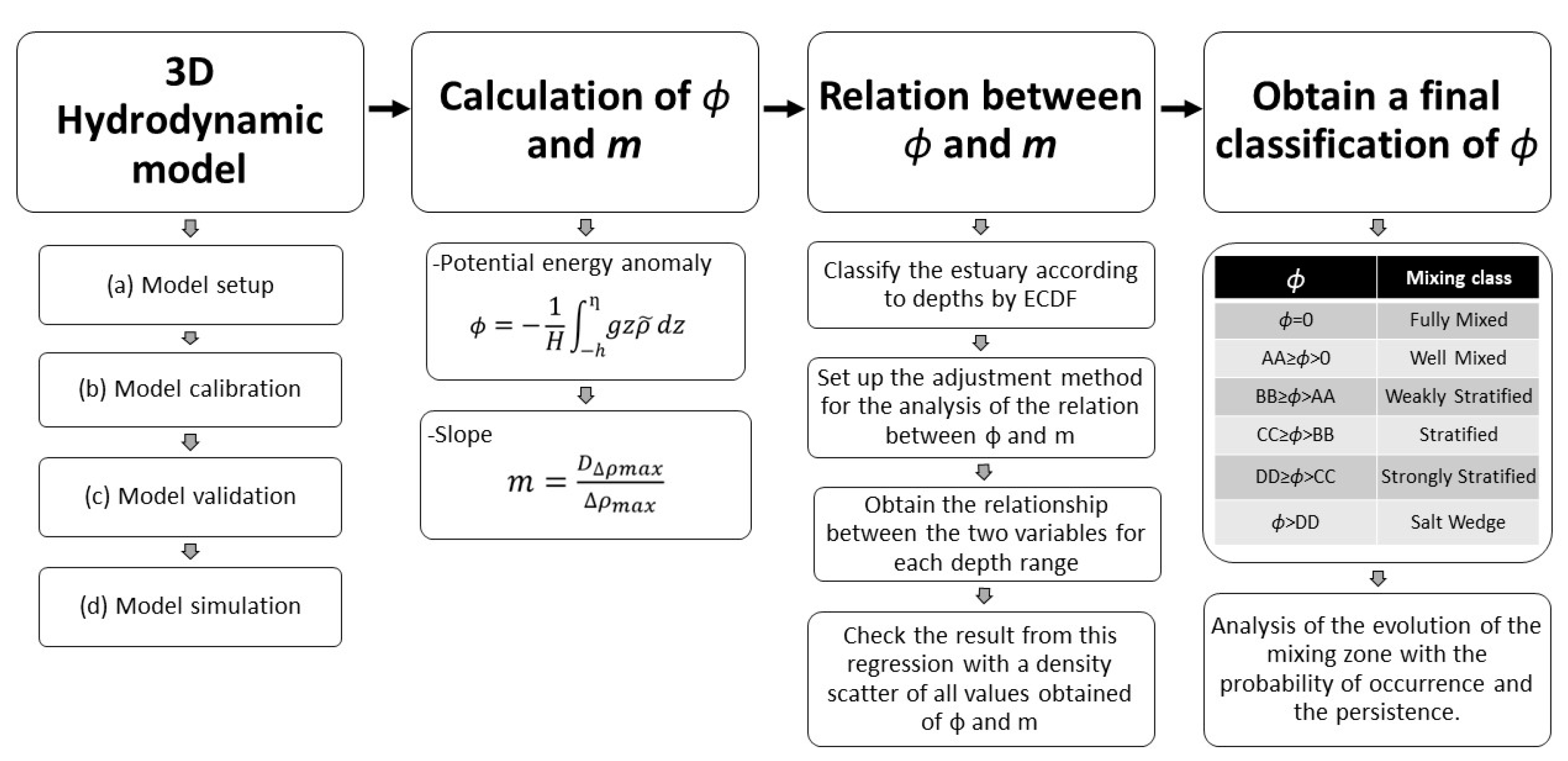
2. Materials and Methods

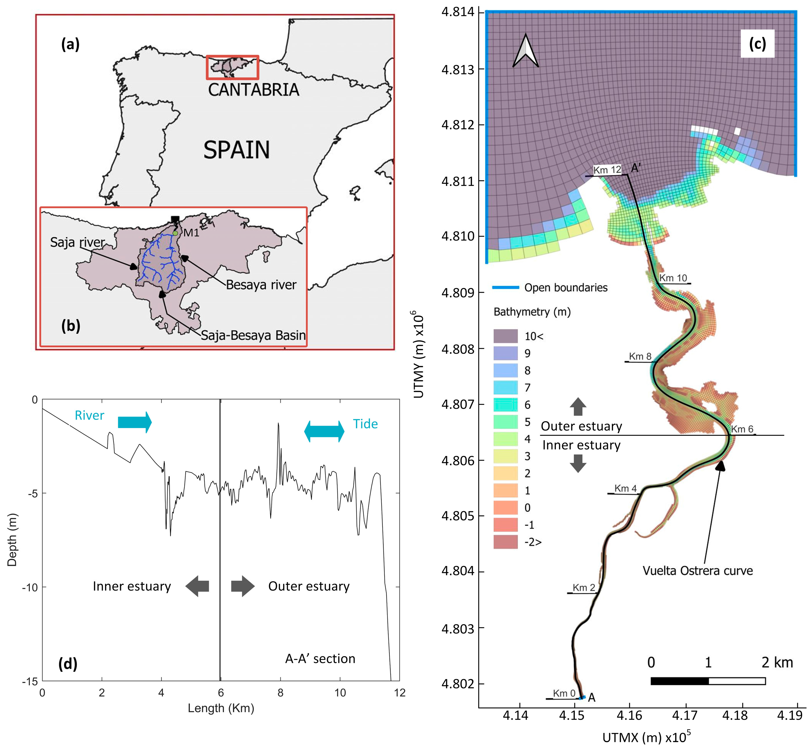
2.1. Study Area and Setup of the 3D Hydrodynamic Model

The Suances estuary (SE) is a mesotidal estuary located on the coast of Cantabria, Spain. With an approximate length of 12 km, an average width of 150 m and a surface area of 339.7 ha, it has intertidal zones that occupy 76% of its surface area. The bathymetry of the study area was obtained from the available nautical charts of the Spanish coast obtained from [33]. This bathymetry was corrected with the data obtained from a field campaign and adjusted in the initial river section to give it a constant slope according to the field observations (see Figure 1). The depth of the main channel varies between 1 m to 8 m, and the intertidal zones rise about 3.2 m above mean sea level. At the adjacent coastal sea, the deepest depth within the study area is 43 m (below the mean sea level) near the northwest corner. Note also that the high resolution of the mesh grid and bathymetry allowed the full definition of dykes bordering the main channel (see Figure 1). For more information on SE, the reader is referred to [10,26,34,35,36].
The 3D hydrodynamic model results obtained by [26] using the interface of the suite of Delft3D-FLOW software in its three-dimension option [37,38,39] has been used to carry out this study. This numerical model is based on finite difference that solves the shallow water equations in three dimensions [40,41]. These equations are derived from the three-dimensional Navier–Stokes equations for free incompressible surface flow. In the case of density, the formulation included in the Delft3D-FLOW software is the international standard formula of UNESCO [42]. The Reynolds stress components are computed using the eddy viscosity concept [43]. The reason for choosing this model is its worldwide use that has confirmed its ability to simulate 3D hydrodynamics in estuaries [3,5,44,45].
The three-dimensional grid, covering the SE and its adjacent coastal zone, was represented horizontally using a curvilinear mesh grid. This mesh grid consisted of 93 × 800 grid cells. The spatial resolution was between 47 and 235 m in the adjacent coastal zone and between 4.3 and 30 m inside the estuary. Regarding the vertical discretization, the mesh grid was composed of 20 vertical σ-layers equally spaced along the water column. The open boundaries of the model correspond to the coastal and river zone (see Figure 1). The tidal forcings (level, temperature and salinity) have been obtained from the Iberian–Biscay–Ireland (IBI) system of Copernicus [46], included in the coastal boundary. For the river boundary, the river flow, temperature and salinity have been calculated by means of a coupled hydrological model specific for this estuary, based on precipitation and air temperature [47]. Finally, a heat flux model has been included to model the interactions of the atmosphere with the free surface of the estuary. This model has been fed with data measured at the meteorological station M1 (Figure 1) (solar irradiance, air temperature and relative humidity) located near the estuary. The time step used in the model was 6 s, recording hourly values of density, velocity, water level, salinity and temperature in each cell and layer of the model.
Once the calibrated and validated model was obtained, it was used to model the hydrodynamics of the year 2020 as the base year. Additionally, four new hydrodynamic projections based on the year 2020 were developed, adapting the forecasts of anomalies due to climate change as new projections in the river forcings (flow and temperature) and coastal forcings (level, temperature and salinity). The scenarios used to analyze the projected changes in the vertical structure were RCP 4.5 and 8.5 for the years 2050 and 2100, respectively. The changes in river forcings have been obtained from [48], a platform for consulting and exchanging information on impacts, vulnerability and adaptation to climate change. The changes in coastal forcings were obtained from the IPCC and NASA sea level rise forecast viewer and the sea temperature estimated from IPCC [49]. Finally, projected salinity was obtained from [50]. For more details about the model set up (time step, numerical scheme, turbulence closure model, etc.), calibration, validation and climate change projections of forcings, readers are referred to [26].

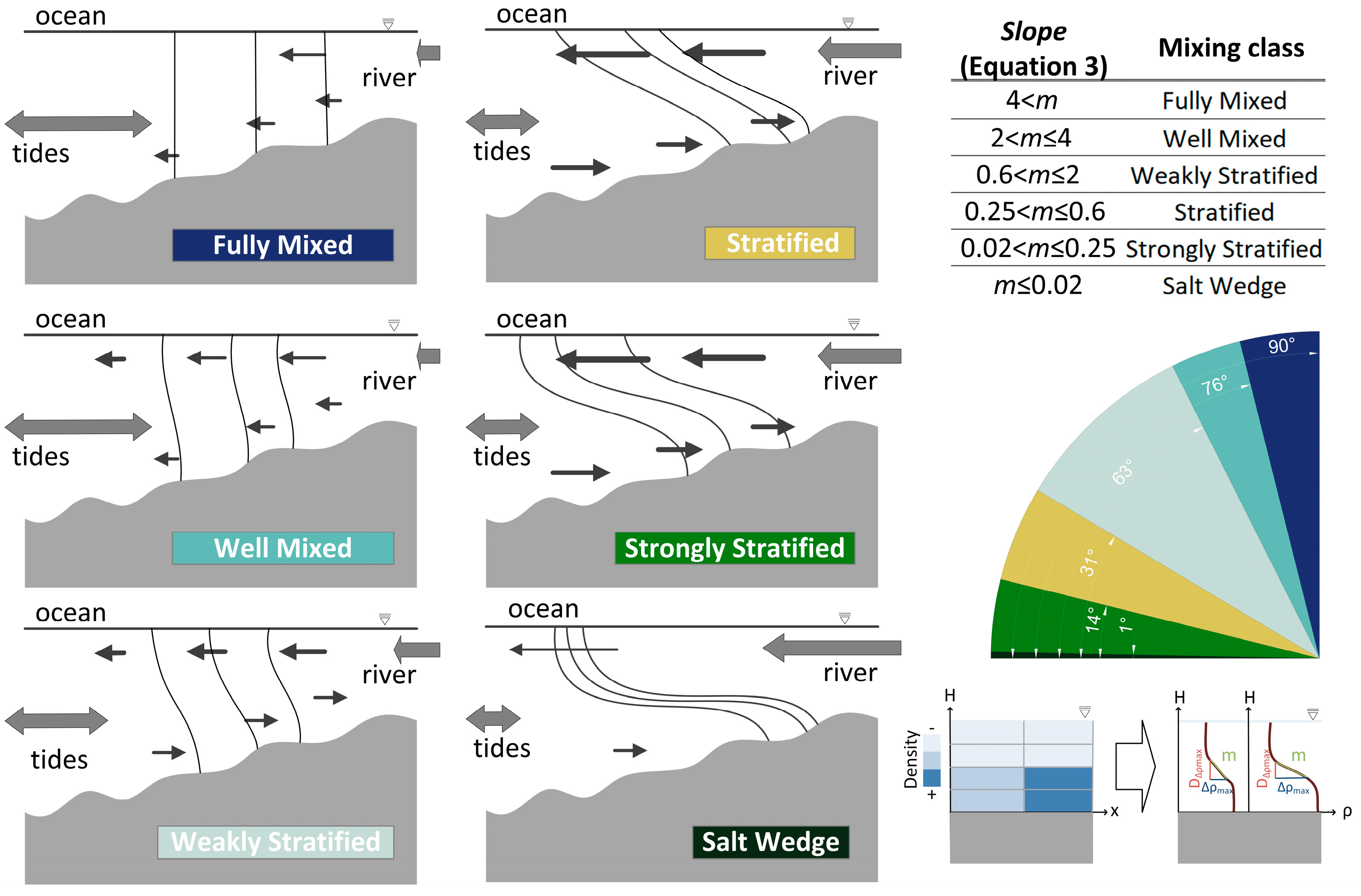
2.2. Classification of the Estuarine Vertical Structure According to the Density Profile Slope ( m )

The parameter m has been selected because it is a physically meaningful parameter that can be easily analyzed by numerical models and field measurements, integrating the competition between mixing versus stratification. The benefit of applying m is that it is possible to create a standardized classification applicable to any estuary in the world, since m does not vary in estuarine systems. Thus, using m, the classification can be established and then related to ϕ that can vary in case-specific estuaries.
First, the calculation of m was defined as in Equation (3). Two methods can be used to calculate this parameter. The first one is based on calculating the minimum slope of the vertical density profiles. This method can be used on density profiles or on field measurements since it only requires knowledge of the vertical density field. The second method, applicable to numerical models, is based on the simplification that in each vertical cell of the model have the same density, which varies linearly between the vertical layers. In this way, it is possible to calculate the maximum difference in density between two layers of the water column (maximum gradient, Δ ρ m a x ) and to find out the distance between layers that this change occurs ( D Δ ρ m a x ). In this way, it is possible to obtain for each model cell a minimum isodeme slope. A calculation scheme is shown in Figure 2.
m = D Δ ρ m a x Δ ρ m a x  
Second, six vertical mixing classes have been proposed, encompassing the terms coined by the previous estuarine classifications of the vertical structure: (1) fully mixed, (2) well mixed, (3) weakly stratified, (4) stratified, (5) strongly stratified and (6) salt wedge. The estuaries reviewed were: Altamaha [51], Cape Fear [17], Columbia [52], Delaware [53], Hudson [14,54], Humber [18], Mandovi [12], Merrimack [2,7], Severn [55], Tomales Bay [56], Ferrol [15], Babitonga bay [57], Oujiang [58], Strymon [59] and Tamar [60]. In all of them, different mixing classes were determined according to the vertical structure. These studies allow us to extrapolate slope ranges for each vertical mixing class by analyzing their m-values.
From this literature review, it has been observed that there is a straightforward relationship between the vertical mixing classes and the density or salinity profile slopes of the water column (whenever salinity is the fundamental parameter affecting density). After the analysis of these data, the slope ranges for each vertical mixing class were established: fully mixed ( 4 < m ), well mixed ( 2 < m 4 ), weakly stratified ( 0.6 < m 2 ), stratified ( 0.25 < m 0.6 ), strongly stratified ( 0.02 < m 0.25 ) and salt wedge ( m 0.02 ).
Figure 2 shows a conceptual model of the density profiles for each vertical mixing class and the proposed slope and/or angle classification. The two extreme cases, fully mixed and salt wedge, have been taken as estuarine areas where the density profiles are practically vertical or horizontal, respectively. The intermediate classes progress from strongly stratified to stratified to weakly stratified and to well mixed, with the profiles becoming steeper due to the different intensities of the main forcings.

2.3. Relationship between the Density Profile Slope and the Potential Energy Anomaly

In order to find the relationship between ϕ-data and m-data, several adjustment methods can be tested to determine which was the most appropriate. It is important to mention that the adjustment method will be unique for each estuary, since it will depend on the nature of the data.
In this study, artificial neural networks (ANN) are used to relate m-data and ϕ-data for every depth range. A neural network is a computing model whose layered structure resembles the interconnected structure of neurons in the brain, with layers of connected nodes. A neural network can learn from data, so it can be trained to recognize patterns and classify data. In this case, the Matlab [61] integrated application Neuronal Network Fitting has been used. This application facilitates the assembly of simple neural networks for implementation and can handle a large amount of data.
For developing an ANN, the first step is to select the network architecture. In this study, the input layer is the m-data, and the output layer corresponds to the ϕ-data. The first calibration parameter will be the number of nodes to be inserted in the hidden layer. Therefore, it is recommended to calibrate the number of nodes that results in the best fit. Next, it is necessary to choose the best transfer function. For instance, this application uses a sigmoid transfer function in the hidden layer and a linear transfer function in the output layer.
As a final step, it is required to find the most suitable network creation method and to define the weights used for training, testing and validation (amount of used data from the total data). In this case, three types of training methods are available: the Levenberg-Marquardt, which optimizes the computations; the Bayesian Regularization, which is slower, but can be used for small or noisy problems and the scaled conjugate Gradient, recommended for settings with large amounts of data, since it is more efficient with memory. The choice of the best method can be determined through a process of iteration, in which the computational cost/benefit is analyzed.
Once the model is executed, it provides output data such as the quadratic errors in each phase (training, testing and validation) as well as the global fitting results and the time taken to fit the model. In addition, these models can be exported, so that the network can be easily used in other codes. For more information on how to set up neural networks, the reader is referred to [62,63].

2.4. Methodology to Classify Mixing Classes According to the Vertical Structure at a Local Scale

The parameter selected for the stratification analysis is the potential energy anomaly (ϕ) introduced by [32] and defined in Equations (1) and (2). However, there is no differentiation between different vertical mixing classes in this parameter, with consideration of only two vertical mixing classes: mixed or stratified when ϕ < 0 or ϕ > 0, respectively. For this reason, this section presents a methodology to classify vertical mixing classes at a local scale based on the density profile slope (m), which allows relating the ϕ-magnitude to a vertical mixing class. This relationship explains the amount of mechanical energy (per m3) required to reach a specific density profile in the water column with a given density profile, i.e., the energy required to reach a vertical mixing class from other vertical mixing classes. For the determination of these parameters, the previously calibrated and validated 3D hydrodynamic model has been used.
The application of this classification to estuaries is performed by the four-tiered method presented in Figure 3. In Tier 1, a 3D hydrodynamic model with high spatial resolution is calibrated and validated (see Section 2.1). Then, in Tier 2, the ϕ and m-values are calculated for every grid cell at each time step. In Tier 3, the relationship between ϕ and m is determined. Lastly, in Tier 4, the ϕ-values are classified into six vertical mixing class by means of the fitted curve and the proposed m-thresholds for every vertical mixing class.
After modeling the selected period in Tier 1 and calculating the magnitude of ϕ and m for every grid cell at each time step in Tier 2, the relationship between ϕ and m is determined in Tier 3. First, the empirical cumulative distribution function (ECDF) of depth is calculated to distinguish between different estuarine zones associated with specific depth ranges influenced by the main forcing conditions (river and sea level). Second, the best adjustment method is selected to relate m-data and ϕ-data for every depth range; for instance, an artificial neural network (ANN) in SE. Lastly, the relationship obtained by the ANNs is checked by performing a density scatter on the vector including all ϕ and m- values.
In Tier 4, the ϕ-values calculated in Tier 2 by using the model results obtained in Tier 1 are classified into six vertical mixing classes by means of the ANNs developed in Tier 3 and the m-thresholds for every vertical mixing class proposed in Section 2.2. Next, the analysis of the spatiotemporal evolution of the estuarine classification is conducted by means of the calculation of two parameters. The first is the probability of occurrence, i.e., the percentage of time that every grid cell is in each class for every time step during the 3D hydrodynamic simulation, obtaining 6 maps of vertical mixing classes, one for each class. These maps integrate the spatiotemporal variability of estuarine stratification along the model simulation period by displaying the frequency of each class. From these probability maps, all the information is integrated into a single map by analyzing which class has the highest probability of occurrence in every grid cell, giving each value a number from 1 to 6. In this way, a map showing the most probable class at local scale is obtained. The second parameter is persistence defined as the maximum time (in hours) that every grid cell is consecutively in each class. Thus, 6 maps are obtained (one for each class) that indicate the spatiotemporal variability for each class in every grid cell. Persistence allows observing patterns of changes, which may be due to the different forcings governing the estuarine mixing behavior.

3. Results

3.1. Relationship between the Density Profile Slope and the Potential Energy Anomaly in the Suances Estuary

The proposed methodology has been applied to the SE during the year 2020 by means of the 3D hydrodynamic model. This year had a total water volume of 780 Hm3, so according to [3], it can be considered a mean year. From this simulation, more than 40 million ϕ and m-values have been obtained: 8785 hourly maps over the year multiplied by every estuarine grid cell. In order to find the relationship between the two sets of data, several adjustment methods have been tested to determine which was the most appropriate. It is important to mention that the adjustment method will be unique for each estuary since it will depend on the nature of the data. To evaluate these data, Pearson’s and Spearman’s coefficients have been calculated to assess whether the available data have linear relationships and if their relation is monotonic, respectively. In this case, coefficients of −0.23 and −0.35 were found, indicating that the relationship between the variables is inverse, the data are not clearly linearly related and the relationship between the data is not monotonic. To achieve more consistent adjustments, ϕ and m data have been grouped into different depths. Therefore, the ECDF of the estuarine depth has been calculated for the simulated year (Figure 4a). From this curve, the estuary has been subdivided into different depth ranges (estuarine zones) according to their breaking points: from 0 to 1 m (tidal marsh zone); from 1 to 4 m (intertidal zone) and higher than 4 m (subtidal zone).
With the data from these three zones, polynomial, exponential, linear, logarithmic and power adjustment methods have been tested, with the objective of evaluating the fits of each and to see how well they fit. The adjustments were not very satisfactory, and therefore it has been necessary to use more complex adjustment methods to find the relationships, since it has been observed that there is a large dispersion of the data that makes a fit with linear or nonlinear models non-reliable.
Filtering the ϕ and m-values for every depth range, three ANNs have been developed with four nodes in the hidden layer, a log sigmoid transfer function, the Levengberg-Marquardt training method and training, validation, and test ratios of 70:15:15, respectively. Table 1 shows the errors obtained from the application of the different adjustment methods.
Once this relationship was obtained, its fit was checked by performing a density scatter including ϕ and m-values for all the grid cells during one year of simulation (Figure 4b–d). As shown in Figure 4, the ANN results fit very precisely to the places where the density of points is highest (black line in Figure 4b–d), presenting R-values from 0.56 to 0.83. Regarding the R-values, it is important to mention that there is a large dispersion when comparing the results, due to the great variability of forcings and mixing situations that can occur, as seen in [26]. In the case of zones with H < 1 m, a total of 1,496,081 data points were compared for each variable, with an R-value of 0.569 for the test, 0.569 for the validation and 0.571 for the training. For 1 m < H < 4 m, 15,278,859 data points for each variable were analyzed, obtaining an R-value of 0.550 for testing, 0.549 for validation and 0.550 for training. Finally, for H > 4 m, 6,174,927 data points for each variable were analyzed, obtaining in this case an R-value of 0.843 for the test, validation and training. Finally, the classification results obtained from the ANNs for every depth range are shown in Table 2.

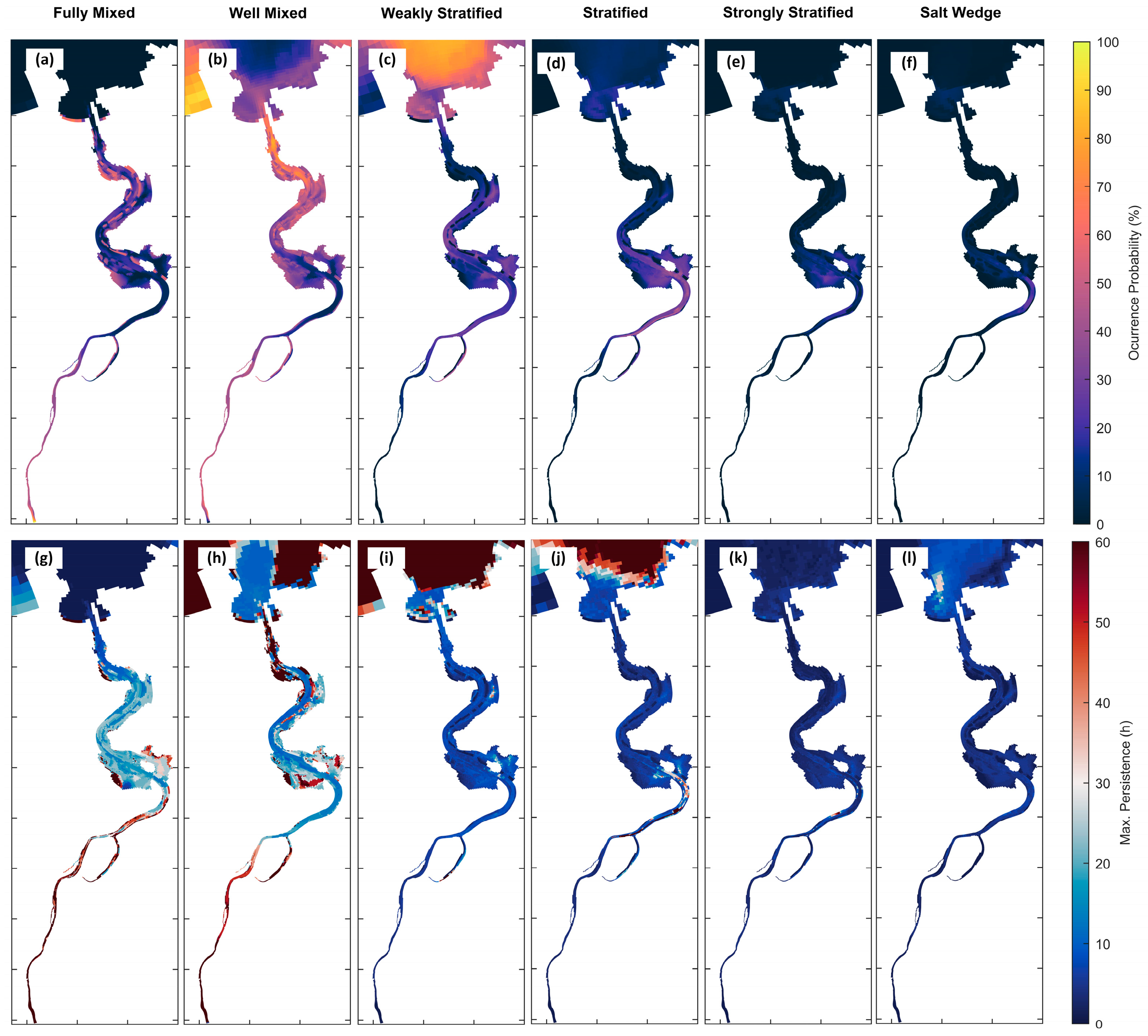
3.2. Spatiotemporal Evolution of Vertical Mixing Classes in the Suances Estuary

Figure 5 shows the occurrence probability and the persistence of each vertical mixing class along the SE as proxies to explain the spatiotemporal evolution of the mixing and stratification processes, using the ϕ-values presented in Table 2. For this purpose, the occurrence probability for every time step (8785) in each grid cell of the estuary has been calculated and then the classification proposed in Table 2 has been applied to the SE. In this way, it has been possible to integrate hourly results for the year 2020 into six maps, one for each vertical mixing class.
As can be seen in Figure 5, the fully mixed class is particularly significant at the estuarine head, where the river influence is greater and the salinity intrusion is negligible. In addition, it is noteworthy that the estuary embankments have been classified as fully mixed, which is why areas of high probability (up to 80%) of this class can be seen along the estuary. The well mixed class is located in the lower part of the estuary near the estuarine mouth, from km 8 to km 11 of the A-A′ section (see Figure 1a,d), presenting zones of occurrence probability higher than 90%. The weakly stratified zone is distributed throughout the estuary, with special relevance in the coastal area outside of the estuarine mouth (75% probability), where the mixing between the estuarine water into the open sea and their advective effects generate this zone of slight stratification. In the case of the stratified class, it occurs in the intermediate zone of the estuary, over the intertidal zone 1 and the “Vuelta Ostrera” curve, where the occurrence probability is around 50%. Finally, salt wedge and strongly stratification classes display a low occurrence probability—<15% in most cases—because they only appear at medium or high river flows. In these situations, it can be observed that the strongly stratified and salt wedge zones are centered in the “Vuelta Ostrera” curve and the adjoining intertidal zones, where the occurrence probability is around 25%.
Regarding the persistence results (see Figure 5), in the case of the fully mixed class, the highest persistence values can be observed in the estuarine head. This upper section has a strong fluvial influence because the water circulating most of the time is fresh water, with a maximum persistence of up to 80 h, coinciding with the duration of the longest river flood event. Conversely, the maximum persistence in the estuarine mouth is 6 h, coinciding with half of a tidal cycle. In the rest of the estuary, the average maximum persistence is 30 h. As for the well mixed class, the variability is low, with a maximum persistence of around 20 h in all the estuary. In the case of the stratified class, the maximum persistence is found in the “Vuelta Ostrera” curve, where values higher than 60 h are observed. Moreover, the weakly stratified class presents a similar trend and persistence to the stratified class. The estuarine head shows a maximum persistence of 20 h, while progressing towards the mouth, the magnitude of the persistence decreases 10 h. Lastly, the strongly stratified and salt wedge classes display the longest persistence at the lower and middle estuarine zones, being around 10 h.
In order to analyze the influence of climate change on the estuary applying the proposed classification, the probability of occurrence and the maximum persistence for the 4 cases analyzed, RCP 4.5 and RCP 8.5 for the years 2050 and 2100, respectively, are shown in Supplementary Material Figures S1–S4. To obtain these maps, the methodology used for Figure 5 was repeated.
In these figures, the fully mixed zones have a slight decrease in the probability of occurrence in all the scenarios, although the highest probability of occurrence is found at the estuarine head. In the case of the well mixed class, a higher probability of occurrence is observed at the estuarine head, especially in the 2100 RCP 8.5 where the probability is 10% higher. This increase in the projected 2100 RCP 8.5 scenario is repeated with the weakly stratified and stratified classes, increasing by about 5%. The strongly stratified class remains similar to 2020 in all projected scenarios. Finally, in the 2050 RCP 4.5 and RCP 8.5 scenarios, the salt wedge class remains in the same probability ranges as the 2020 scenario—around 25% in the “Vuelta Ostrera” curve. However, in the 2100 RCP 4.5 and RCP 8.5 scenarios, this probability is reduced to below 5% throughout the estuary.
In terms of persistence, the fully mixed class displays a decrease for the projected 2100 RCP 4.5 and RCP 8.5 scenarios in the middle zone of the estuary, before the curve of “Vuelta Ostrera”, lowering its persistence from 20 h to 10 h (drop to 50%). In the case of the well mixed class, the persistence in the intertidal zone 1 has values of around 70 h for the 2020 scenario and the projected RCP 4.5 scenarios. However, in the projected RCP 8.5 scenarios for both the years 2050 and 2100, this persistence drops from 42% to around 30 h. For the stratified class, higher persistence values are obtained around the “Vuelta Ostrera”, which, unlike the 2020 scenario, occupies the entire width of the main channel with persistence above 80 h for the four projected scenarios, 130% higher than for the 2020 scenario. In the rest of the classes, persistence remains unchanged. It is noteworthy how the projected RCP 8.5 scenarios tend to have around 5% higher persistence than the projected RCP 4.5 scenarios for both the years 2050 and 2100, which may be due to the decrease in the intensity of the forcings due to climate change, which decreases the variability of the classes.
Finally, Figure 6 shows the most probable vertical mixing classes in the SE by integrating the occurrence probability of each vertical mixing class into a single map. Panels Figure 6a,b present the results for the 2020 scenario, panels Figure 6c,d the 2050 RCP 4.5 scenario, panels Figure 6e,f the 2050 RCP 8.5 scenario, panels Figure 6g,h the 2100 RCP 4.5 scenario and panels Figure 6i,j the 2100 RCP 85 scenario. Additionally, panels Figure 6a,c,e,g,i present the outer part of the estuary (see Figure 1a,d) while the panels Figure 6b,d,f,h,j present the inner part of the estuary (see Figure 1a,d).
In the 2020 scenario, the estuarine head (from km 0 to km 1 of the A-A′ section (see Figure 1a,d)), which is directly influenced by the river, is usually fully mixed. Next, there is a zone which is well mixed, located before intertidal zone 1 (km 6 of the A-A′ section (see Figure 1a,d)). Down the estuary, it is possible to find the most probable stratification zone of the estuary, taking the “Vuelta Ostrera” curve and part of the intertidal zone 1. After this, there is a new zone of well mixed classification that goes from the middle to the lower estuarine zones, from km 8 to 12 of the A-A′ section (see Figure 1a,d). At the estuarine mouth, the most likely vertical mixing class is weakly stratified. This weakly stratified class can be caused by the discharge of estuarine water (brackish water) into the open sea (salt water).
For the projected climate change scenarios, the SE presents a high spatiotemporal variability of the mixing and stratification processes. As shown in the projected 2050 scenarios, the stratification zones are located in places like those of the 2020 scenario, between km 4 and km 8 of the A-A′ section (see Figure 1a,d). However, in the projected four scenarios, the fully mixed areas tend to disappear from km 6 to km 12 of the A-A′ section (see Figure 1a,d), especially in intertidal areas, being replaced by well mixed class.
On the other hand, in the projected 2100 RCP 4.5 scenario, the stratification zones have expanded in the intertidal zone and main channel, from km 4 to km 2 of the A-A′ section (see Figure 1a,d). Although, in the projected 2100 RCP 8.5 scenario, there is a displacement of areas classified as stratified upstream of the estuary, due to the change in forcing, more pronounced in the scenarios projected for 2100 [26].

4. Discussion

4.1. Relationship between Vertical Structure and Density Slopes to Establish Vertical Mixing Classes

As noted in Section 2.3, a literature review has been carried out in order to find an objective estuarine classification based on density profile slopes. Table 3 shows the density profile slopes calculated for every graph shown in the searched works.
As can be seen in Table 3, each author names the vertical mixing classes in a different manner, without apparently having a clear and concise term. With the proposed classification, most of the terms coined in the literature are encompassed, with the possibility of homogenizing the terms in the future, so that the scientific community can use the same terminology and avoid confusion between terms. Although the proposed classification covers most of the references analyzed and agrees with the given vertical mixing classes, there are situations where the vertical mixing classes proposed by the new classification differs from the given vertical mixing classes. The main reason is that there is no specific classification for naming the vertical mixing classes, nor a rule that indicates what can be considered one class or another, so each author subjectively chooses one class. The aim of this proposal is to deal with this problem, so that a homogeneous way of naming and classifying the mixing classes is presented according to the vertical structure of the water column.

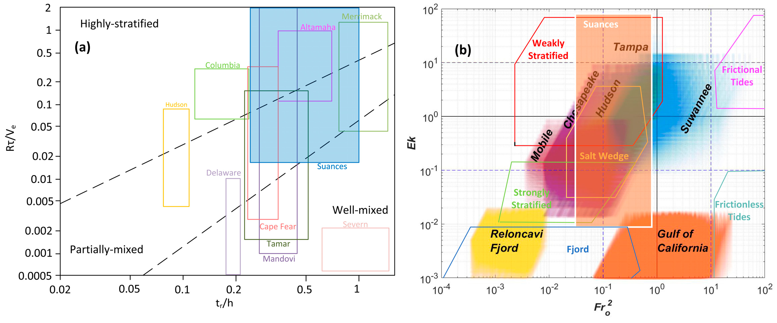
4.2. Classification of the Suances Estuary Using Other Methodologies

To compare the results obtained in the SE with the proposed classification, the methodologies described in [24,25] have been applied. On the one hand, using [24] for the maximum and minimum runoff and tidal range, it is possible to classify an estuary in three vertical mixing classes: highly stratified, partially mixed (or partially stratified) and well mixed. On the other hand, for applying [25], it is necessary to obtain the Ekman and tidal Froude numbers. To carry out both calculations, the model results from the year 2020 have been used. The results of applying these methodologies can be seen in Figure 7.
As can be seen in Figure 7, the SE is placed within all the vertical mixing classes, since, as has been seen throughout this work, the estuarine classification varies spatially and temporally according to their vertical structure. Both classifications agree very closely with the results obtained using the new methodology. Therefore, the SE is a highly variable estuary in both classifications, varying between well mixed and highly stratified in [24] and between weakly stratified and salt wedge in [25]. It is noteworthy that both classifications are made with values of extreme and minimum situations, so that on most occasions, the representation of our estuary will focus on average events. In the case of ordinary flow events, low or medium discharge, the estuary is classified as weakly stratified or partially mixed and well mixed. According to the analysis carried out in this study, it matches quite reliably, as the estuary has been categorized most of the time in a well mixed to stratified class. Nevertheless, in the event of a high flow event, areas of strong stratification or even salt wedge occur, coinciding with both classifications described in this section.

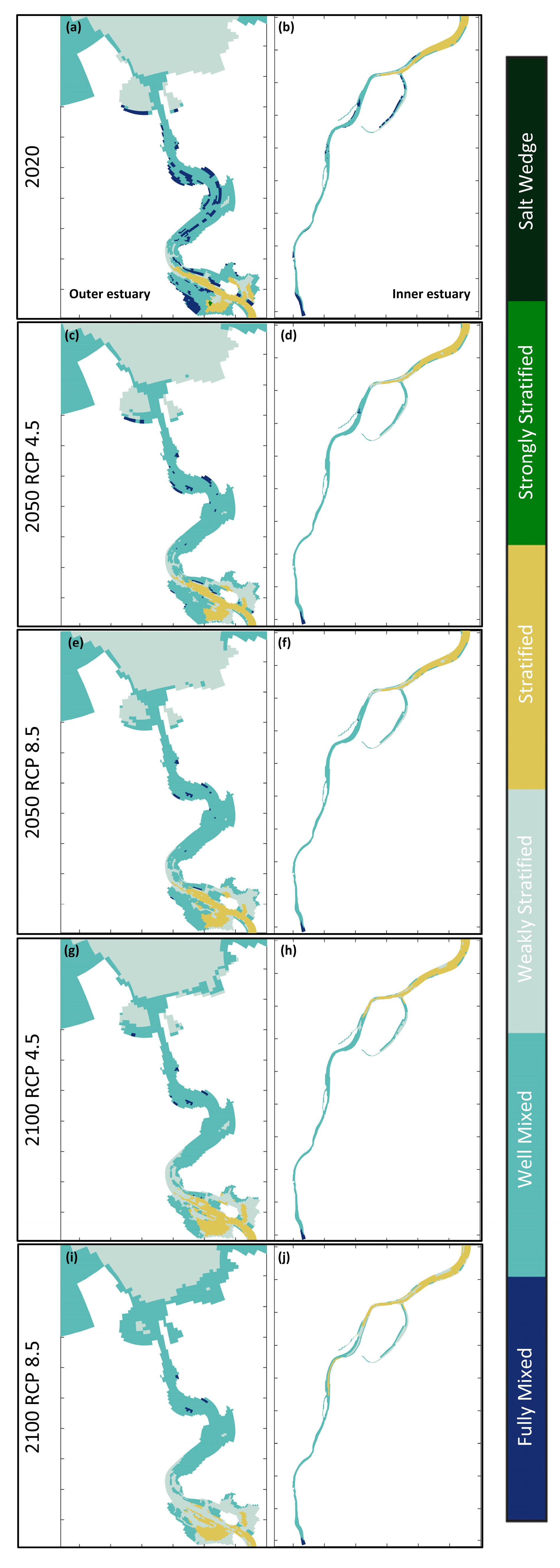
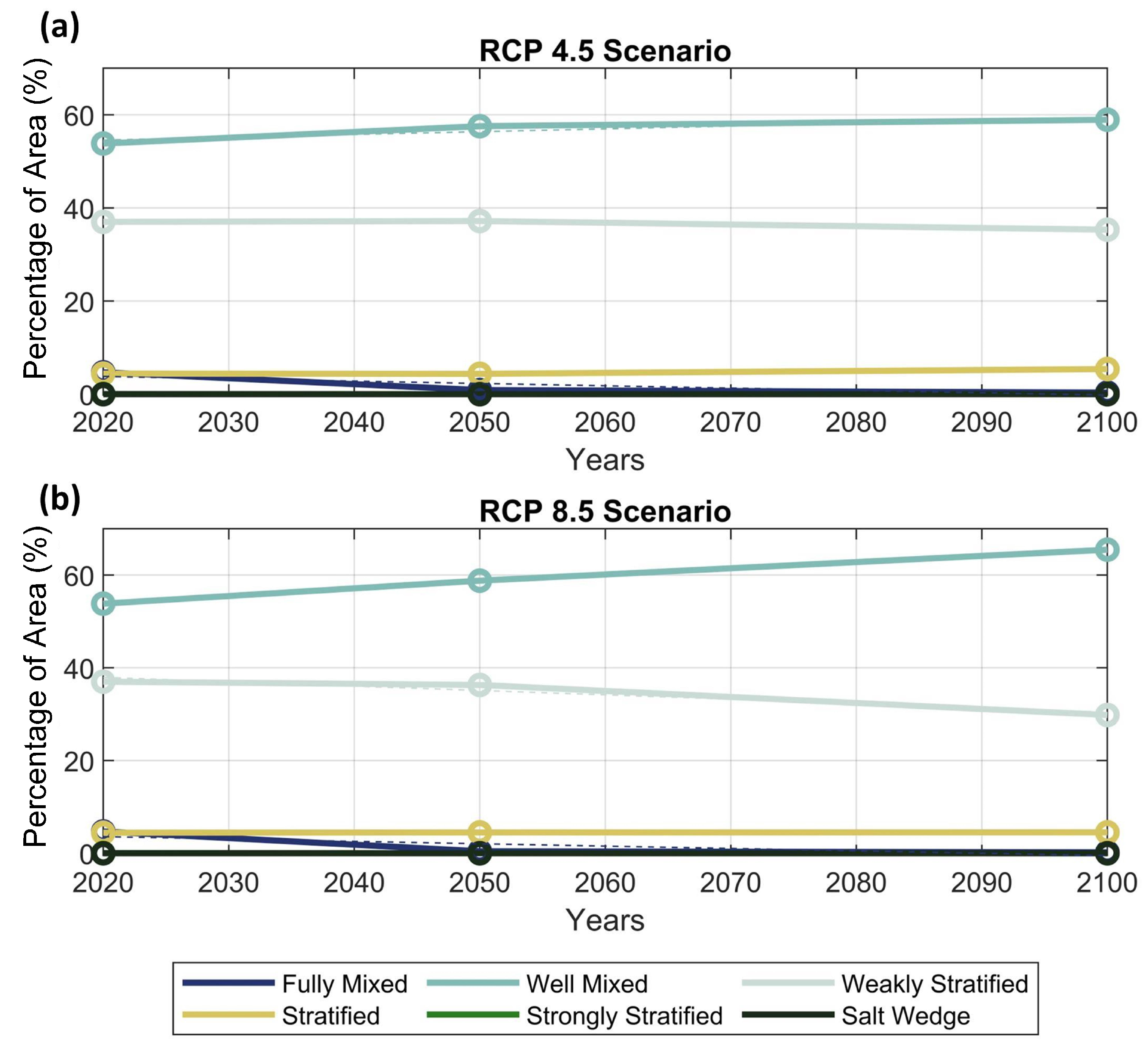
4.3. Dynamic Classification of Estuarine Vertical Structure and Projected Modifications under Climate Change

As was mentioned, this study has focused on estuaries where astronomical tides and river discharges are the most important forcing factors explaining the stratification and mixing variability. These types of estuaries are distributed worldwide, so a methodology to classify their vertical mixing classes as well as their potential modifications due to climate change could help researchers, technicians and/or policymakers to diagnose potential issues more efficiently.
With large intertidal zones, large changes in river flows and a highly variable tidal range, the vertical mixing of these estuaries primarily depend on the tide, which determines the spatial variation of the mixing zone with its rise and descent (ebb–flood cycle). The regulation of mixing and stratification is modulated in time by the spring–neap cycle, as described by [64]. In addition, the spring–neap cycle affects the length and location of the mixing fronts [26]. However, when a river flood occurs, these extraordinary contributions of freshwater flush move the mixing zone towards the estuarine mouth and can even move all the brackish water in the estuary seaward if, at the same time, river flood events occur with ebb tides. This behavior has recently been reported in other estuaries [59,65]. In the case of SE, this can be attributed to the dominance of both river flow and tidal flow during the river flood events with higher control of river flow over the tidal flow because the SE geometry (small estuary) is highly sensitive to the water volume introduced into the system.
Figure 8 shows the percentage of area in each vertical mixing class for the climate change projections in the RCP 4.5 (a) and RCP 8.5 (b) scenarios. Through this figure it is possible to observe the trend of each vertical mixing class.
As shown in Figure 8, the most probable vertical mixing class of SE in the 2020 scenario is well mixed because of low flow contributions during most of the year, which means that areas of high stratification cannot occur. However, weakly stratified zones are observed at the mouth of the estuary and in the intertidal zones, because of estuarine water outflowing to the sea. On the other hand, in the intermediate zone of the estuary there is a zone classified as stratified, where the confluence between seawater and river water usually occurs. Finally, the only areas classified as fully mixed are found upstream of the estuary, where the river enters the estuary and where the tide is not usually present, and in the levee, areas scattered throughout the estuary.
Climate change projections show a significant decrease in the areas classified as fully mixed, from 4.7% for the 2020 scenario to 0.9%, 0.4%, 0.3% and 0.2% for the RCP 4.5 and RCP 8.5 scenarios for the years 2050 and 2100, respectively. The sea level rise will increase the depths, reducing the tidal marshal zones, making mixing and stratification processes in these areas more likely to occur. The reason behind these causes is the fact that sea level rise will increase the water column, and therefore create more pronounced stratification patterns back inland from the estuary as seen in the various studies analyzed in the region surrounding the study area, such as the NW Atlantic coast of Portugal [66,67] or the UK coast [68]. This is especially noticeable in the intertidal zones, where in the 2020 scenario there were fully mixed zones that have now been replaced by weakly stratified zones. On the other hand, In the well mixed zones, there is a clear increase in their presence, with the most probable area of this state reaching 53.8% in 2020 and 65.5% in the RCP 8.5 scenario in the year 2100. This result is in line with what was observed in [26], where it was seen that the decrease in flow will reduce the mixing zones, and these will move further upstream. As far as the weakly stratified class is concerned, no significant changes are observed in percentage of area, with all scenarios in the range of 37%, except in the RCP 8.5 scenario of 2100, which drops to 29.8% due to this more significant decrease in river inputs. Finally, the area classified as stratified remains constant at around 4.5% in all scenarios, although as the projections progress, this area tends to move upstream of the estuary.
Equation (4) and Table 4 present the linear trends calculated for each vertical mixing class as a percentage of the estuarine area in each class. It is noteworthy that no analysis has been conducted regarding strongly stratified and salt wedge classes, as these classes only have a local influence in certain high flow events (>50 m3/s), being insignificant in a whole year study (0.03% of the area of strongly stratified class for the 2020 scenario and 0% for strongly stratified and salt wedge in the four projected scenarios).
P r o j e c t e d   %   o f   a r e a = a P r o j e c t e d   y e a r + b
To apply Equation (4), the vertical mixing class to be analyzed can be selected and the parameters listed in Table 3 can be used to obtain a projection in the selected year.
As shown in Figure 8, the fully mixed and weakly stratified zones tend to disappear because their m-terms are negative for both scenarios (RCP 4.5 and RCP 8.5). Moreover, it can be observed that this trend is similar in both scenarios. This may be associated with a decreased freshwater inflow to the estuary and increased tidal excursion along the estuary, producing a shift of the river/estuarine front upstream of the zones in line with the results observed by [69], which leads to the fully mixed zones disappearing. On the other hand, there is an increase in the number of zones classified as well mixed, especially in the RCP 8.5 scenario. Finally, the zones classified as stratified tend to remain the same or increase slightly in the RCP 4.5 scenario.

5. Conclusions

In a modern-day Tower of Babel, an ever-increasing confusion has been caused by terminology, use and estimation of vertical mixing classes, despite valuable efforts towards a sounder theoretical framework. Therefore, this study presents a proposal for the homogenization of the terminology used to define these vertical mixing classes based on an easily interpretable physical variable such as the density of the water column. With this, it is possible to quantify vertical mixing classes based on the slopes of the density profile (m) and its relationship with the potential energy anomaly (ϕ). This physical approach, based on the slope of the density profile and relating it to the potential energy anomaly, makes it easy to implement, unlike other classifications that require the estimation or assumption of certain parameters that are difficult to measure or calculate.
Finally, the values of the potential energy anomaly have been quantified like other widely used parameters, such as the Richardson number. The magnitude of the potential energy anomaly has been classified in ranges that have not been found to date to link potential energy anomaly with vertical mixing classes. This could lead to better understanding and applicability of this parameter.
As far as the Suances estuary is concerned, it can be seen how in the 2020 scenario the zones classified as well mixed were predominant in the estuary, occupying 53.8% of the area, and how these vertical mixing class will grow in the projected scenarios up to 20%. On the other hand, there is a decrease of between 5% (2050 RCP 4.5 scenario) and 20% (2100 RCP 8.5 scenario) in the zones classified as weakly stratified. Additionally, there is a decrease of around 90% in the zones classified as fully mixed, showing how the estuary will tend towards homogenization in the well mixed class because of climate change. Regarding the strongly stratified and salt wedge classes, no relevance is observed at the annual scale. However, the influence of the strongly stratified and salt wedge classes is significant in specific high flow events (>50 m3/s), where these vertical mixing classes occur. Finally, it is remarkable how the decrease in the forcings as well as the rise in sea level makes the areas classified as stratified tend to move upstream of the estuary, displacing the starting point from km 4 to km 2 of the A-A′ section (see Figure 1a,d).
Finally, the application of artificial neural networks to the Suances estuary has allowed the relation of the large amount of available data (>40 million values) of the potential energy anomaly and the water column density slope, giving relationships that fit very closely to the realistic distributions, with values of R ranging from 0.57 to 0.83. The use of artificial neural networks in this study has proved successful and gives reason to extend their use in other fields of application when it is necessary to relate a large amount of data with nonlinear relationships.

Supplementary Materials

The following supporting information can be downloaded at: https://www.mdpi.com/article/10.3390/w15183294/s1. Figure S1. Occurrence probability (a–f) and maximum persistence in hours (g–l) for each vertical mixing class in the Suances estuary: fully mixed (a,g); well mixed (b,h); weakly stratified (c,i); stratified (d,j); strongly stratified (e,k) and salt wedge (f,l) for the 2050 RCP 4.5 scenario. Figure S2. Occurrence probability (a to f) and maximum persistence in hours (g–l) for each vertical mixing class in the Suances estuary: fully mixed (a,g); well mixed (b,h); weakly stratified (c,i); stratified (d,j); strongly stratified (e,k) and salt wedge (f,l) for the 2050 RCP 8.5 scenario. Figure S3. Occurrence probability (a–f) and maximum persistence in hours (g–l) for each vertical mixing class in the Suances estuary: fully mixed (a,g); well mixed (b,h); weakly stratified (c,i); stratified (d,j); strongly stratified (e,k) and salt wedge (f,l) for the 2100 RCP 4.5 scenario. Figure S4. Occurrence probability (a–f) and maximum persistence in hours (g–l) for each vertical mixing class in the Suances estuary: fully mixed (a,g); well mixed (b,h); weakly stratified (c,i); stratified (d,j); strongly stratified (e,k) and salt wedge (f,l) for the 2100 RCP 8.5 scenario.

Author Contributions

Conceptualization, J.L. and J.F.B.; methodology, J.L. and J.F.B.; software, J.L.; validation, J.L.; formal analysis, J.L. and J.F.B.; investigation, J.L. and J.F.B.; resources, J.L. and J.F.B.; data curation, J.L. and J.F.B.; writing—original draft preparation, J.L.; writing—review and editing, J.F.B., J.G.-A. and A.G.; visualization, J.L.; supervision, J.F.B.; project administration, A.G.; funding acquisition, J.L. and A.G. All authors have read and agreed to the published version of the manuscript.

Funding

This research was funded by PID2021-127358NB-I00-MCIN/AEI/10.13039/501100011033 and by FEDER as a way of making Europe. Moreover, the research was also funded by RTI2018-095304-B-I00-MCIU/AEI/FEDER,UE. Finally, this study was also financed by the 2i program of the Provincial Council of Bizkaia (Spain) with expedient number 6/12/2i/2019/153.

Data Availability Statement

Data are available on request due to privacy restrictions. The data presented in this study are available on request from the corresponding author. The data are not publicly available due to these data are being used in our subsequent research efforts.

Conflicts of Interest

The authors declare no conflict of interest.

References

  1. Simpson, J.H.; Hughes, D.G.; Morris, N.C.G. The relation of seasonal stratification to tidal mixing on the continental shelf. Deep-Sea Res. 1977, 24, 327–340. [Google Scholar]
  2. Geyer, W.; Scully, M.; Ralston, D. Quantifying vertical mixing in estuaries. Environ. Fluid Mech. 2008, 8, 495–509. [Google Scholar] [CrossRef]
  3. Bárcena, J.F.; Camus, P.; García, A.; Álvarez, C. Selecting model scenarios of real hydrodynamic forcings on mesotidal and macrotidal estuaries influenced by river discharges using K-means clustering. Environ. Model. Softw. 2015, 68, 70–82. [Google Scholar] [CrossRef]
  4. Zhang, R.; Hong, B.; Zhu, L.; Gong, W.; Zhang, H. Responses of estuarine circulation to the morphological evolution in a 1 convergent, microtidal estuary. Ocean Sci. 2022, 18, 213–231. [Google Scholar] [CrossRef]
  5. Couceiro, M.A.; Schettini, C.A.; Siegle, E. Modeling an arrested salt-wedge estuary subjected to variable river flow. Reg. Stud. Mar. Sci. 2021, 47, 101993. [Google Scholar] [CrossRef]
  6. Khadami, F.; Kawanisi, K.; Al Sawaf, M.B.; Gusti, G.N.N.; Xiao, C. Spatiotemporal Response of Currents and Mixing to the Interaction of Tides and River Runoff in a Mesotidal Estuary. Ocean Sci. J. 2022, 57, 37–51. [Google Scholar] [CrossRef]
  7. Ralston, D.K.; Geyer, W.R.; Lerczak, J.A. Structure, variability, and salt flux in a strongly forced salt wedge estuary. J. Geophys. Res. Atmos. 2010, 115, C06005. [Google Scholar] [CrossRef]
  8. Rijnsburger, S.; Flores, R.P.; Pietrzak, J.D.; Horner-Devine, A.R.; Souza, A.J. The Influence of Tide and Wind on the Propagation of Fronts in a Shallow River Plume. J. Geophys. Res. Oceans 2018, 123, 5426–5442. [Google Scholar] [CrossRef]
  9. Ross, L.; Valle-Levinson, A.; Sottolichio, A.; Huybrechts, N. Lateral variability of subtidal flow at the mid-reaches of a macrotidal estuary. J. Geophys. Res. Oceans 2017, 122, 7651–7673. [Google Scholar] [CrossRef]
  10. Bárcena, J.F.; García, A.; García, J.; Álvarez, C.; Revilla, J. Surface analysis of free surface and velocity to changes in river flow and tidal amplitude on a shallow mesotidal estuary: An application in Suances Estuary (Nothern Spain). J. Hidrology 2012, 420, 301–308. [Google Scholar] [CrossRef]
  11. García, A.; Juanes, J.A.; Álvarez, C.; Revilla, J.A.; Medina, R. Assesment of the response of a shallow macrotidal estuary to changes in hydrological and wastewater inputs through numerical modelling. Ecol. Model. 2010, 221, 1194–1208. [Google Scholar] [CrossRef]
  12. Vijith, V.; Sundar, D.; Shetye, S. Time-dependence of salinity in monsoonal estuaries. Estuar. Coast. Shelf Sci. 2009, 85, 601–608. [Google Scholar] [CrossRef]
  13. Buschman, F.A.; Hoitink, A.J.F.; van der Vegt, M.; Hoekstra, P. Subtidal water level variation controlled by river flow and tides. Water Resour. Res. 2009, 45, 601–608. [Google Scholar] [CrossRef]
  14. Warner, J.C.; Geyer, W.R.; Lerczak, J.A. Numerical modeling of an estuary: A comprehensive skill assessment. J. Geophys. Res. Atmos. 2005, 110, C5. [Google Scholar] [CrossRef]
  15. Decastro, M.; Gomez-Gesteira, M.; Prego, R.; Alvarez, I. Ria–ocean exchange driven by tides in the Ria of Ferrol (NW Spain). Estuar. Coast. Shelf Sci. 2004, 61, 15–24. [Google Scholar] [CrossRef]
  16. Geyer, W.R.; Ralston, D.K.; Chen, J. Mechanisms of Exchange Flow in an Estuary with a Narrow, Deep Channel and Wide, Shallow Shoals. J. Geophys. Res. Oceans 2020, 125, e2020JC016092. [Google Scholar] [CrossRef]
  17. Becker, M.L.; Luettich, R.A., Jr.; Mallin, M.A. Hydrodynamic behavior of the Cape Fear River and estuarine system: A synthesis and observational investigation of discharge–salinity intrusion relationships. Estuar. Coast. Shelf Sci. 2010, 88, 407–418. [Google Scholar] [CrossRef]
  18. Uncles, R.; Stephens, J.; Law, D. Turbidity maximum in the macrotidal, highly turbid Humber Estuary, UK: Flocs, fluid mud, stationary suspensions and tidal bores. Estuar. Coast. Shelf Sci. 2006, 67, 30–52. [Google Scholar] [CrossRef]
  19. Du, J.; Park, K.; Shen, J.; Dzwonkowski, B.; Yu, X.; Yoon, B.I. Role of Baroclinic Processes on Flushing Characteristics in a Highly Stratified Estuarine System, Mobile Bay, Alabama. J. Geophys. Res. Oceans 2018, 123, 4518–4537. [Google Scholar] [CrossRef]
  20. Pritchard, D. Estuarine hydrography. Adv. Geophys. 1952, 1, 243–280. [Google Scholar] [CrossRef]
  21. Hansen, D.V.; Rattray, M. New dimensions in estuary classification. Limnol. Oceanogr. 1966, 11, 319–326. [Google Scholar] [CrossRef]
  22. Geyer, W.R.; MacCready, P. The Estuarine Circulation. Annu. Rev. Fluid Mech. 2014, 46, 175–197. [Google Scholar] [CrossRef]
  23. Guha, A.; Lawrence, G.A. Estuary Classification Revisited. J. Phys. Oceanogr. 2013, 43, 1566–1571. [Google Scholar] [CrossRef]
  24. Vijith, V.; Shetye, S. A stratification prediction diagram from characteristics of geometry, tides and runoff for estuaries with a prominent channel. Estuar. Coast. Shelf Sci. 2012, 98, 101–107. [Google Scholar] [CrossRef]
  25. Valle-Levinson, A. Dynamics-based classification of semienclosed basins. Reg. Stud. Mar. Sci. 2021, 46, 101866. [Google Scholar] [CrossRef]
  26. Lupiola, J.; Bárcena, J.F.; García-Alba, J.; García, A. A numerical study of the mixing and stratification alterations in estuaries due to climate change using the potential energy anomaly. Front. Mar. Sci. 2023, 10, 1206006. [Google Scholar] [CrossRef]
  27. Yang, F.; Ji, X.; Zhang, W.; Zou, H.; Jiang, W.; Xu, Y. Characteristics and Driving Mechanisms of Salinity Stratification during the Wet Season in the Pearl River Estuary, China. J. Mar. Sci. Eng. 2022, 10, 1927. [Google Scholar] [CrossRef]
  28. Zhang, J.; Cheng, L.; Wang, Y.; Jiang, C. The Impact of Tidal Straining and Advection on the Stratification in a Partially Mixed Estuary. Water 2023, 15, 339. [Google Scholar] [CrossRef]
  29. Yamaguchi, R.; Suga, T.; Richards, K.J.; Qiu, B. Diagnosing the development of seasonal stratification using the potential energy anomaly in the North Pacific. Clim. Dyn. 2019, 53, 4667–4681. [Google Scholar] [CrossRef]
  30. Lenoch, L.K.; Survey, U.G.; Stumpner, P.R.; Burau, J.R.; Loken, L.; Sadro, S. Dispersion and Stratification Dynamics in the Upper Sacramento River Deep Water Ship Channel. San Fr. Estuary Watershed Sci. 2021, 19, 1–29. [Google Scholar] [CrossRef]
  31. Hamada, T.; Kim, S. Stratification potential-energy anomaly index standardized by external tide level. Estuar. Coast. Shelf Sci. 2021, 250, 107138. [Google Scholar] [CrossRef]
  32. Simpson, J.H.; Crisp, D.J.; Hearn, C. The shelf-sea fronts: Implications of their existence and behaviour. Philos. Trans. R. Soc. Lond. Ser. A Math. Phys. Sci. 1981, 302, 531–546. [Google Scholar] [CrossRef]
  33. González, M.; Medina, R.; Gonzalez-Ondina, J.; Osorio, A.; Méndez, F.J.; García, E. An integrated coastal modeling system for analyzing beach processes and beach restoration projects, SMC. Comput. Geosci. 2007, 33, 916–931. [Google Scholar] [CrossRef]
  34. Bárcena, J.F.; García, A.; Gómez, A.G.; Álvarez, C.; Juanes, J.A.; Revilla, J.A. Spatial and temporal flushing time approach in estuaries influenced by river and tide. An application in Suances Estuary (Northern Spain). Estuar. Coast. Shelf Sci. 2012, 112, 40–51. [Google Scholar] [CrossRef]
  35. Bárcena, J.F.; García-Alba, J.; García, A.; Álvarez, C. Analysis of stratification patterns in river-influenced mesotidal and macrotidal estuaries using 3D hydrodynamic modelling and K-means clustering. Estuar. Coast. Shelf Sci. 2016, 181, 1–13. [Google Scholar] [CrossRef]
  36. Bárcena, J.F.; Gómez, A.G.; García, A.; Álvarez, C.; Juanes, J.A. Quantifying and mapping the vulnerability of estuaries to point-source pollution using a multi-metric assessment: The Estuarine Vulnerability Index (EVI). Ecol. Indic. 2017, 76, 159–169. [Google Scholar] [CrossRef]
  37. Nicholson, J.; Broker, I.; Roelvink, J.A.; Price, D.; Tanguy, J.M.; Moreno, L. Intercomparison of coastal area morphodynamic models. Coast. Eng. 1997, 31, 97–123. [Google Scholar] [CrossRef]
  38. Lesser, G.R.; Roelvink, J.A.; van Kester, J.A.; Stelling, G.S. Development and validation of a three-dimensional morphological model. Coast. Eng. 2004, 51, 883–915. [Google Scholar] [CrossRef]
  39. Chung, T. Computational Fluid Dynamics; Cambridge University Press: Cambridge, UK, 2002; 1012p. [Google Scholar]
  40. Stelling, G. On the Construction of Computational Methods for Shallow Water Flow Problems. Ph.D. Thesis, TUDelft, Delft, The Netherlands, 1983. Available online: http://resolver.tudelft.nl/uuid:d3b818cb-9f91-4369-a03e-d90c8c175a96 (accessed on 6 July 2021).
  41. Stelling, G.; Leendertse, I. Approximation of Convective Processes by Cyclic ADI Methods. In Proceedings of the 11th International Conference on Estuarine and Coastal Modeling, American Society of Civil Engineers, Reston, VA, USA; 1991; pp. 771–782. [Google Scholar]
  42. UNESCO. Background papers and supporting data on the international equation of state. Tech. Rep. UNESCO 1981, 31, 174. [Google Scholar]
  43. Rodi, W. Examples of calculation methods for flow and mixing in stratified fluids. J. Geophys. Res. Atmos. 1987, 92, 5305–5328. [Google Scholar] [CrossRef]
  44. García-Alba, J.; Gómez, A.; Sámano, M.; García, A.; Juanes, J. A 3-d model to analyze environmental effects of dredging operations–application to the port of Marin, Spain. Adv. Geosci. 2014, 39, 95–99. Available online: http://hdl.handle.net/10902/4596 (accessed on 10 December 2022). [CrossRef]
  45. Jiménez, M.; Castanedo, S.; Zhou, Z.; Coco, G.; Medina, R.; Rodriguez-Iturbe, I. Scaling properties of tidal networks. Water Resour. Res. 2014, 50, 4585–4602. [Google Scholar] [CrossRef]
  46. Sotillo, M.G.; Cailleau, S.; Lorente, P.; Levier, B.R.; Aznar, R.; Reffray, G.; Amo-Baladrón, A.; Chanut, J.; Benkiran, M.; Alvarez-Fanjul, E. The MyOcean IBI Ocean Forecast and Reanalysis Systems: Operational products and roadmap to the future Copernicus Service. J. Oper. Oceanogr. 2015, 8, 63–79. [Google Scholar] [CrossRef]
  47. Álvarez, C.; Garcia, E.; Prieto, C.; Rojo, J.; Tejerina, B. Aplicación de un modelo logístico triparamétrico a la estimación de caudales diarios en la cuenca del río Nam Ngum (Laos). In Proceedings of the IV Jornadas de Ingeniería del Agua: “La Precipitación y los Procesos Erosivos”, Córdoba, Spain, 21–22 October 2015; Volume B.8, pp. 255–268. [Google Scholar]
  48. OECC. Fundación Biodiversidad Visor de escenarios de cambio climático de AdapteCCa. Available online: http://escenarios.adaptecca.es (accessed on 10 December 2022).
  49. IPCC. Summary for Policymakers. In IPCC Special Report on the Ocean and Cryosphere in a Changing Climate; Po, H.-O., Roberts, D.C., Masson-Delmotte, V., Zhai, P., Tignor, M., Poloczanska, E., Mintenbeck, K., Alegría, A., Nicolai, M., Okem, A., et al., Eds.; Cambridge University Press: Cambridge, UK; New York, NY, USA, 2019; pp. 3–35. [Google Scholar] [CrossRef]
  50. Skliris, N.; Marsh, R.; Mecking, J.V.; Zika, J.D. Changing water cycle and freshwater transports in the Atlantic Ocean in observations and CMIP5 models. Clim. Dyn. 2020, 54, 4971–4989. [Google Scholar] [CrossRef]
  51. Kang, K.R.; Di Iorio, D. Depth- and current-induced effects on wave propagation into the Altamaha River Estuary, Georgia. Estuar. Coast. Shelf Sci. 2007, 66, 395–408. [Google Scholar] [CrossRef]
  52. Jay, D.A.; Smith, J.D. Residual circulation in shallow estuaries: Highly stratified estuaries, narrow estuaries. J. Geophys. Res. Atmos. 1990, 95, 711–731. [Google Scholar] [CrossRef]
  53. Cook, T.L.; Sommerfield, C.K.; Wong, K.-C. Observations of tidal and springtime sediment transport in the upper Delaware Estuary. Estuar. Coast. Shelf Sci. 2007, 72, 235–246. [Google Scholar] [CrossRef]
  54. Geyer, W.R.; Trowbridge, J.H.; Bowen, M.M. The Dynamics of a Partially Mixed Estuary. J. Phys. Oceanogr. 2000, 30, 2035–2048. [Google Scholar] [CrossRef]
  55. Uncles, R.J. Physical properties and processes in the Bristol Channel and Severn Estuary. Mar. Pollut. Bull. 2010, 61, 5–20. [Google Scholar] [CrossRef]
  56. Harcourt-Baldwin, J.-L.; Diedericks, G. Numerical modelling and analysis of temperature controlled density currents in Tomales Bay, California. Estuar. Coast. Shelf Sci. 2006, 66, 417–428. [Google Scholar] [CrossRef]
  57. Noernberg, M.A.; Rodrigo, P.A.; Luersen, D.M. Seasonal and fortnightly variability of the hydrodynamic regime at Babitonga Bay, Southern of Brazil. Reg. Stud. Mar. Sci. 2020, 40, 101518. [Google Scholar] [CrossRef]
  58. Xing, Y.; Ai, C.; Jin, S. A three-dimensional hydrodynamic and salinity transport model of estuarine circulation with an application to a macrotidal estuary. Appl. Ocean Res. 2013, 39, 53–71. [Google Scholar] [CrossRef]
  59. Zachopoulos, K.; Kokkos, N.; Sylaios, G. Salt wedge intrusion modeling along the lower reaches of a Mediterranean river. Reg. Stud. Mar. Sci. 2020, 39, 101467. [Google Scholar] [CrossRef]
  60. Grabemann, I.; Uncles, R.J.; Krause, G.; Stephens, J.A. Behaviour of Turbidity Maxima in the Tamar (U.K.) and Weser (F.R.G.) Estuaries. Estuar. Coast. Shelf Sci. 1997, 45, 235–246. [Google Scholar] [CrossRef]
  61. The MathWorks Inc. MATLAB. (2022); Version 9.12.0 (R2022a); The MathWorks Inc.: Natick, MA, USA, 2022; Available online: https://www.mathworks.com (accessed on 10 December 2022).
  62. García-Alba, J.; Bárcena, J.F.; Ugarteburu, C.; García, A. Artificial neural networks as emulators of process-based models to analyse bathing water quality in estuaries. Water Res. 2019, 150, 283–295. [Google Scholar] [CrossRef]
  63. García-Alba, J.; Bárcena, J.F.; Pedraz, L.; Fernández, F.; García, A.; Mecías, M.; Costas-Veigas, J.; Samano, M.L.; Szpilman, D. SOSeas Web App: An assessment web-based decision support tool to predict. J. Oper. Oceanogr. 2021, 16, 155–174. [Google Scholar] [CrossRef]
  64. MacCready, P.; Geyer, W.R.; Burchard, H. Estuarine Exchange Flow Is Related to Mixing through the Salinity Variance Budget. J. Phys. Oceanogr. 2018, 48, 1375–1384. [Google Scholar] [CrossRef]
  65. Otero, L.J.; Hernandez, H.I.; Higgins, A.E.; Restrepo, J.C.; Álvarez, O.A. Interannual and seasonal variability of stratification and mixing in a high-discharge micro-tidal delta: Magdalena River. J. Mar. Syst. 2021, 224, 103621. [Google Scholar] [CrossRef]
  66. Pereira, H.; Sousa, M.C.; Vieira, L.R.; Morgado, F.; Dias, J.M. Modelling Salt Intrusion and Estuarine Plumes under Climate Change Scenarios in Two Transitional Ecosystems from the NW Atlantic Coast. J. Mar. Sci. Eng. 2022, 10, 262. [Google Scholar] [CrossRef]
  67. Menten, G.; Melo, W.; Pinho, J.; Iglesias, I.; Carmo, J.A.D. Simulation of Saltwater Intrusion in the Minho River Estuary under Sea Level Rise Scenarios. Water 2023, 15, 2313. [Google Scholar] [CrossRef]
  68. Robins, P.E.; Skov, M.W.; Lewis, M.J.; Giménez, L.; Davies, A.G.; Malham, S.K.; Neill, S.P.; McDonald, J.E.; Whitton, T.A.; Jackson, S.E.; et al. Impact of climate change on UK estuaries: A review of past trends and potential projections. Estuar. Coast. Shelf Sci. 2016, 169, 119–135. [Google Scholar] [CrossRef]
  69. Ma, M.; Zhang, W.; Chen, W.; Deng, J.; Schrum, C. Impacts of morphological change and sea-level rise on stratification in the Pearl River Estuary. Front. Mar. Sci. 2023, 10, 1072080. [Google Scholar] [CrossRef]
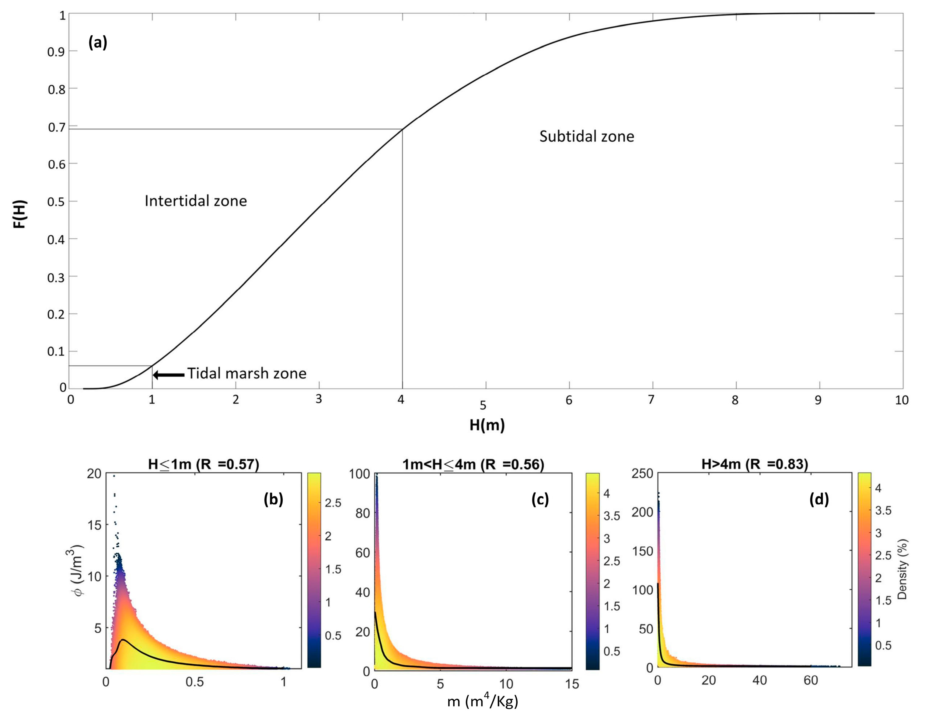
Figure 1. (a) Location of Cantabria in Spain and (b) the Saja-Besaya river basin, (c) bathymetry used in the 3D hydrodynamic model, the model mesh grid and the open boundaries and (d) longitudinal section of the Suances estuary (A-A′ profile).
Water 15 03294 g001
Figure 2. Proposed estuarine classification according to their vertical structures based on the density profile slopes and their graphical representation. The six left panels represent each of the proposed vertical mixing classes. Right panels from top to bottom: (1) classification and denomination of the proposed vertical mixing classes; (2) representation of the slope gradients in degrees; (3) graphical explanation of how m is calculated.
Water 15 03294 g002
Figure 3. Methodology to obtain the relationship between the density profile slope and the potential energy anomaly.
Water 15 03294 g003
Figure 4. Results of the ANN adjustment. (a) ECDF function of the depths of each estuarine cell over the simulated period and the proposed depth ranges to distinguish between estuarine zones; density scatter of the ϕ and m-values from the results obtained from the model simulation and curve fitted by ANNs (black lines) in the tidal marsh zone (b), intertidal zone (c) and subtidal zone (d).
Water 15 03294 g004
Figure 5. Occurrence probability (af) and maximum persistence in hours (gl) for each vertical mixing class in the Suances estuary: fully mixed (a,g); well mixed (b,h); weakly stratified (c,i); stratified (d,j); strongly stratified (e,k) and salt wedge (f,l).
Water 15 03294 g005
Figure 6. Most probable vertical mixing class in the Suances estuary during: (a,b) the year 2020; (c,d) 2050 RCP 4.5; (e,f) 2050 RCP 8.5; (g,h) 2100 RCP 4.5 and (i,j) 2100 RCP 8.5 climate change scenarios. The outer part of the estuary (see Figure 1a,d) is shown in panels (a,c,e,g,i) and the inner part of the estuary (see Figure 1a,d) is shown in panels (b,d,f,h,j).
Water 15 03294 g006
Figure 7. Variability of vertical mixing classes in the Suances estuary based on the diagram proposed by (a) [24] and (b) [25]. Figure adapted with permission from Ref. [24], 2021, Elsevier and from Ref. [25], 2021, Elsevier.
Water 15 03294 g007
Figure 8. Percentage of area in each vertical mixing class from analyzing a full year of results for: (a) RCP 4.5 and (b) RCP 8.5. Dashed lines indicate the interpolation of the results.
Water 15 03294 g008
Table 1. Adjustment methods used with the errors of each one of them.
Adjustment MethodR (H ≤ 1 m)R (1 m < H ≤ 4 m)R (H > 4 m)
Polynomial0.310.230.29
Exponential0.310.290.69
Linear0.270.150.19
Logarithmic0.300.260.55
Power0.280.250.68
ANN0.570.560.83
Table 2. Proposed potential energy anomaly classification in the SE.
Vertical Mixing Classesϕ (H ≤ 1 m)ϕ (1 m < H ≤ 4 m)ϕ (H > 4 m)
Fully Mixedϕ = 0ϕ = 0ϕ = 0
Well Mixed0 < ϕ ≤ 1.00 < ϕ ≤ 2.70 < ϕ ≤ 8.3
Weakly Stratified1.0 < ϕ ≤ 1.22.7 < ϕ ≤ 9.88.3 < ϕ ≤ 34.1
Stratified1.2 < ϕ ≤ 2.19.8 < ϕ≤ 19.434.1 < ϕ ≤ 70.1
Strongly Stratified2.1 < ϕ19.4 < ϕ ≤ 29.970.1 < ϕ ≤ 104.7
Salt Wedge-29.9 < ϕ104.7 < ϕ
Table 3. Analysis of the estuarine slopes with the terms used in their works, calculated as the maximum slope of each density or salinity profile, and the comparison with the classification proposed in this study.
EstuaryReferenceSlopeLiterature ClassificationProposed Classification
Altamaha[51]3.6MixedWell Mixed
0.63Weakly StratifiedWeakly Stratified
0.05Strongly StratifiedStrongly Stratified
0.15Highly StratifiedStrongly Stratified
Babitonga bay[57]0.95Weakly StratifiedWeakly Stratified
0.92Weakly StratifiedWeakly Stratified
0.33StratifiedStratified
0.34StratifiedStratified
Cape Fear[17]0.39Partially MixedStratified
0.48Partially MixedStratified
0.56Partially MixedStratified
0.47Partially MixedStratified
Columbia[52]3Weakly StratifiedWell Mixed
3Weakly StratifiedWell Mixed
4.25Weakly StratifiedFully Mixed
0.35Substantial StratificationStratified
0.66Substantial StratificationWeakly Stratified
0.53Substantial StratificationStratified
Delaware[53]8.5MixedFully Mixed
2.48Weakly StratifiedWell Mixed
28MixedFully Mixed
4Weakly StratifiedWeakly Stratified
0.22Weakly StratifiedStrongly Stratified
Hudson[54]0.24StratifiedStrongly Stratified
[14]0.22Strongly StratifiedStrongly Stratified
1.02Weakly StratifiedWeakly Stratified
Humber[18]2.1Well MixedWell Mixed
9.75Well MixedFully Mixed
Mandovi[12]21Well MixedFully Mixed
13.83Well MixedFully Mixed
0.09Salt WedgeStrongly Stratified
0.19Salt WedgeStrongly Stratified
1.82Partially MixedWeakly Stratified
6.66Well MixedFully Mixed
Merrimack[7]0.15Strongly StratifiedStrongly Stratified
0.19Strongly StratifiedStrongly Stratified
0.18Strongly StratifiedStrongly Stratified
0.24StratifiedStrongly Stratified
0.63StratifiedStratified
0.35StratifiedStratified
[2]0.18Highly StratifiedStrongly Stratified
Oujiang[58]7.6Well MixedFully Mixed
7.95Well MixedFully Mixed
6.6Well MixedFully Mixed
1.88Well MixedWeakly Stratified
0.34Partial MixedStratified
0.45Partial MixedStratified
Ria Ferrol[15]6.6Well MixedFully Mixed
Severn[55]18.6Well MixedFully Mixed
Strymon[59]0.02Salt WedgeSalt Wedge
0.027Salt WedgeStrongly Stratified
0.015Salt WedgeSalt Wedge
0.016Salt WedgeSalt Wedge
Tamar[60]0.1StratifiedStrongly Stratified
Tomales Bay[56]0.29StratifiedStratified
Table 4. Quantification of climate change effect according to RCP 4.5 and RCP 8.5 projections on the percentage of estuarine area modified for every vertical mixing class.
Vertical Mixing ClassesRCP 4.5RCP 8.5
abRabR
Fully mixed−0.05104.810.85−0.0509106.40.81
Well mixed0.0601−66.8340.920.1443−237.421.00
Weakly stratified−0.022783.2770.89−0.0939227.60.96
Stratified0.013−22.0550.910.00092.61450.90
Disclaimer/Publisher’s Note: The statements, opinions and data contained in all publications are solely those of the individual author(s) and contributor(s) and not of MDPI and/or the editor(s). MDPI and/or the editor(s) disclaim responsibility for any injury to people or property resulting from any ideas, methods, instructions or products referred to in the content.

