Article

Towards Adaptive Water Management—Optimizing River Water Diversion at the Basin Scale under Future Environmental Conditions

1
Department of Computational Landscape Ecology, Helmholtz-Centre for Environmental Research—UFZ, 04318 Leipzig, Germany
2
IHCantabria—Instituto de Hidráulica Ambiental, Universidad de Cantabria, 39011 Santander, Spain
*
Author to whom correspondence should be addressed.
Water 2023, 15(18), 3289; https://doi.org/10.3390/w15183289
Submission received: 28 July 2023 / Revised: 11 September 2023 / Accepted: 15 September 2023 / Published: 18 September 2023
(This article belongs to the Special Issue Integrated Water Resources Modeling and Management)

Abstract

:
The degree of success of river water diversion planning decisions is affected by uncertain environmental conditions. The adaptive water management framework incorporates this uncertainty at all stages of management. While the most effective form of adaptive management requires experimental comparison of practices, the use of optimization modeling is convenient for conducting exploratory simulations to evaluate the spatiotemporal implications of current water diversion management decisions under future environmental changes. We demonstrate such an explorative modeling approach by assessing river water availability for diversion in a river basin in Northern Spain under two future environmental scenarios that combine climate and land use change. An evolutionary optimization method is applied to identify and reduce trade-offs with Supporting Ecosystem Services linked to environmental flow requirements for relevant local freshwater species. The results show that seasonal shifts and spatial heterogeneity of diversion volumes are the main challenges for the future diversion management of the Pas River. Basin-scale diversion management should take into account the seasonal planning horizon and the setting of tailored diversion targets at the local-level to promote the implementation of adaptive management. The presented assessment can help with strategic placement of diversion points and timing of withdrawals, but it also provides deeper insight into how optimisation can support decision-making in managing water diversion under uncertain future environmental conditions.

1. Introduction

The “natural flow paradigm” [1] is acknowledged as the basic concept for a thriving river ecosystem; however, recognizing that certain key flow components must be conserved presents a unique challenge for managing river water resources sustainably. Currently, the challenges related to water resource management and its allocation are increasing each year globally due to several pressures, such as climate change and population growth, but also due to trade and energy crises, food production, water scarcity, and pandemics, to name a few [2,3]. In Europe, there are significant differences between countries in terms of both the intensity of the pressures mentioned above, especially climate change extremes [4], and the degree of effectiveness of the water management strategies employed [5]. Enhancing water management efficiency requires anticipating the consequences of management outcomes and future environmental circumstances. To achieve this, we need advanced modeling approaches that can assess and guide decision-making in current and future scenarios.
The water management encompasses a range of interventions aimed at regulating the river system, which involve constructing dams to control water flow or diverting river water. Through water intakes, water diversion alters the flow regime of the river (i.e., its magnitude, seasonality, and variability) [6], potentially compromising the integrity and functionality of the river ecosystem and the services it provides [7,8,9,10,11,12,13]. The concept of environmental or ecological flows (e-flows) is recognized as a valuable instrument for achieving sustainable water resource management or sustainable water diversion, as it considers the ‘quantity, quality and timing of flows that are needed to sustain the ecosystem’ [10,14]. The ongoing intensification of environmental changes related to climate and land use leads to uncertainty in the timing and location of river flow components alteration manifestation (i.e., e-flows). As a consequence, modeling approaches providing means for exploring spatiotemporal implications of current water diversion management decisions under future environmental changes could provide water managers with reliable information for strategic water diversion planning [15,16,17,18,19].
The water diversion management strategies implemented so far are, to some extent, supported by the incorporation of the Integrated Water Resource Management (IWRM) concept [20,21]. While the latter remains a cornerstone of water management approaches, it has evolved into a more articulated paradigm: the “adaptive” water management based on the “learning by doing” cycle, which better meets the need to deal with the increasing uncertainty associated with future changes and management outcomes [20,21,22,23,24]. While a management strategy or decision is assessed in the outer loop, uncertainty within the cycle is addressed through inner loops of minor adjustments to the management approach as functional outcomes become available (for a detailed explanation, see: [16,25]). However, this inherently implies that adaptive management of water resources involves implementing a particular management strategy and repeatedly adjusting it to achieve the desired success or management objective. Indeed, “the most effective form of adaptive management employs management programs that are designed to experimentally compare selected policies or practices by evaluating alternative hypotheses about the system being managed” [26,27]. However, comparing policies and practices in the actual world is time- and resource-consuming and not very cost-effective, making it highly unlikely. Nevertheless, using models that consider real-world conditions to conduct experimental simulations allows these hypotheses to be tested before implementation takes place. Moreover, this approach enables the identification of space and time dimensions that would enable the implementation of an adaptive management cycle.
Many modeling approaches to predict water management outcomes under uncertainty are available nowadays [19,28,29,30,31,32]. Modeling and simulating are generally subject to uncertainties arising from various sources (see [19,32]). One way to tackle the uncertainty associated with water diversion management outcomes is to evaluate management decisions under different environmental change scenarios. Optimization modeling is a versatile tool for this purpose and has been used extensively to model water-management problems [33,34]. It represents a prescriptive type of modeling [30] and is flexible in terms of the type, size, and scale of the problem but does not require extensive training compared to using software. Ultimately, optimization is suitable for analyzing solutions to water-management problems through the employment of system perceptions (i.e., real-world system representation as we perceive it to be), preferences (i.e., preferred solutions based on personal interests and priorities), and scenarios (i.e., plausible real-world conditions) [33,35].
Optimization has been used in studies assessing changes in riparian areas at the river network segment scale [36]; however, the authors are not aware that an optimization assessment has been carried out for river water diversion at each segment of a river basin network considering future environmental changes. To bridge this gap, in this paper, we performed an optimization assessment for the Pas River basin in Northern Spain. Through this study, we aimed to showcase the applicability of the optimization approach at the river network scale with river segment resolution. More specifically, the modeling exercise aimed to (1) design an optimization model for river flow diversion and ecosystem services (ES) supply capacity at the basin scale under climate and land use change scenarios, (2) identify spatial and temporal patterns in the optimization results, and (3) provide recommendations for basin-scale water diversion management and modeling to relevant experts. The presented approach was designed to consider local hydrological conditions and plausible future scenarios while addressing the environmental flow requirements of key biological groups (i.e., Supporting ES). The assessment performed with the presented approach aimed to identify spatiotemporal scales that increase the robustness of current diversion management decisions to climate and land-use changes, with the ultimate goal of facilitating the identification of scales that enable adaptive management.
The paper is organized as follows: Section 2 introduces the case study and the framework of the optimization problem (Section 2.1 and Section 2.2) through the stages of problem perception and problem definition. A suite of representative results is presented in Section 3. Section 4 discusses the spatial and temporal scales of change. Based on the explorative modeling assessment, we provided recommendations for both management and modeling (Section 5).
Using the case application example, this study provides greater insight into how optimization can support decision-making on water diversion management under uncertain future environmental conditions. Moreover, it further supports the identification of temporal and spatial scales relevant to the implementation of an adaptive approach for diversion management planning at the basin scale, while also highlighting the importance of incorporating instream ecological requirements into model development.

2. Materials and Methods

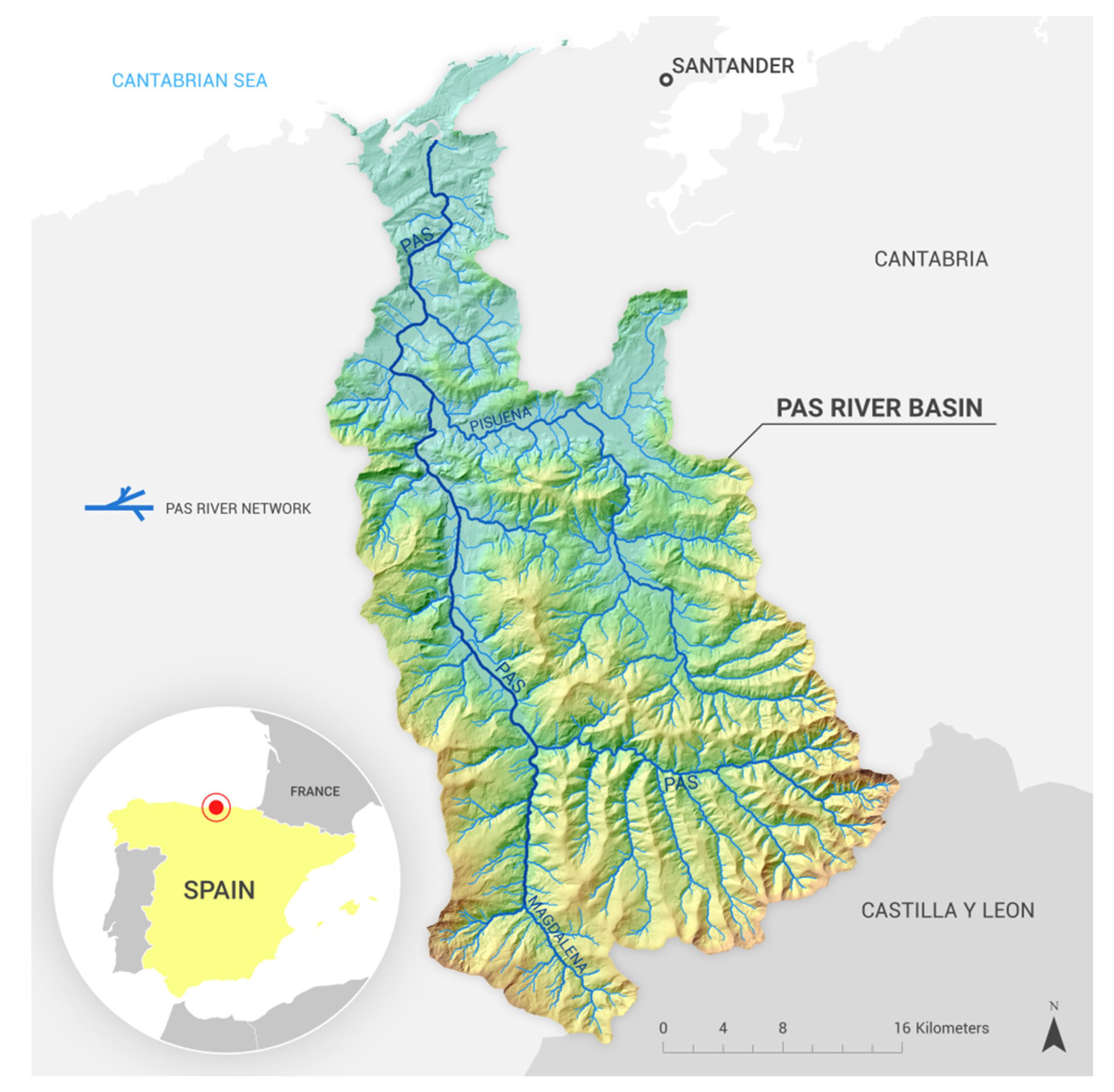
2.1. The Pas River Basin

The Pas River basin (Figure 1) is located in the North of Spain (Cantabrian region) and covers an area of 650 km2 (approx.) with an average elevation of 446 m. The Pas River is characterized by a length of 57 km and a mean slope of 34%. Its network comprises three main rivers (Pas, Pisueña, and Magdalena) that drain into the Cantabrian Sea (Northeast Atlantic). With a mean annual precipitation of 1300 mm, the region’s temperate climate provides significant precipitation throughout the year, generating a mean annual daily flow of 14 m3/s close to the river mouth. The river supplies drinking water to the population of the different municipalities in the region, including the metropolitan area of Santander (>170,000 inhabitants) and its surroundings. Water abstraction from the Pas River is carried out by daily diversion of river surface water (by cross-channel weirs and pumps) at multiple locations throughout the network to satisfy bid-based municipal water allocations. Moreover, the Pas River is the habitat for iconic species such as the Atlantic salmon or the EU-protected alder-ash riparian forests. It is expected that increasing human water demands and changing environmental conditions, such as reduced forest cover in the catchment, reduced precipitation, and higher temperatures from climate change, will lead to growing pressure on the ecological integrity of the Pas River ecosystem [37,38]. The intensification of these drivers can affect the provision of essential Ecosystem Services (ES) in the whole basin, such as those related to regulating and maintaining key ecological processes, conditions, and habitats (i.e., Supporting ES). In this study, a set of 230 target sites (i.e., individual river segments with a maximum length of 500 m, hereafter referred to as RS) were extracted from the cartographic information of the river network data by considering only river segments that were of stream order ≥ 4. Each RS of the set considered in the assessment carries individual hydrological information.

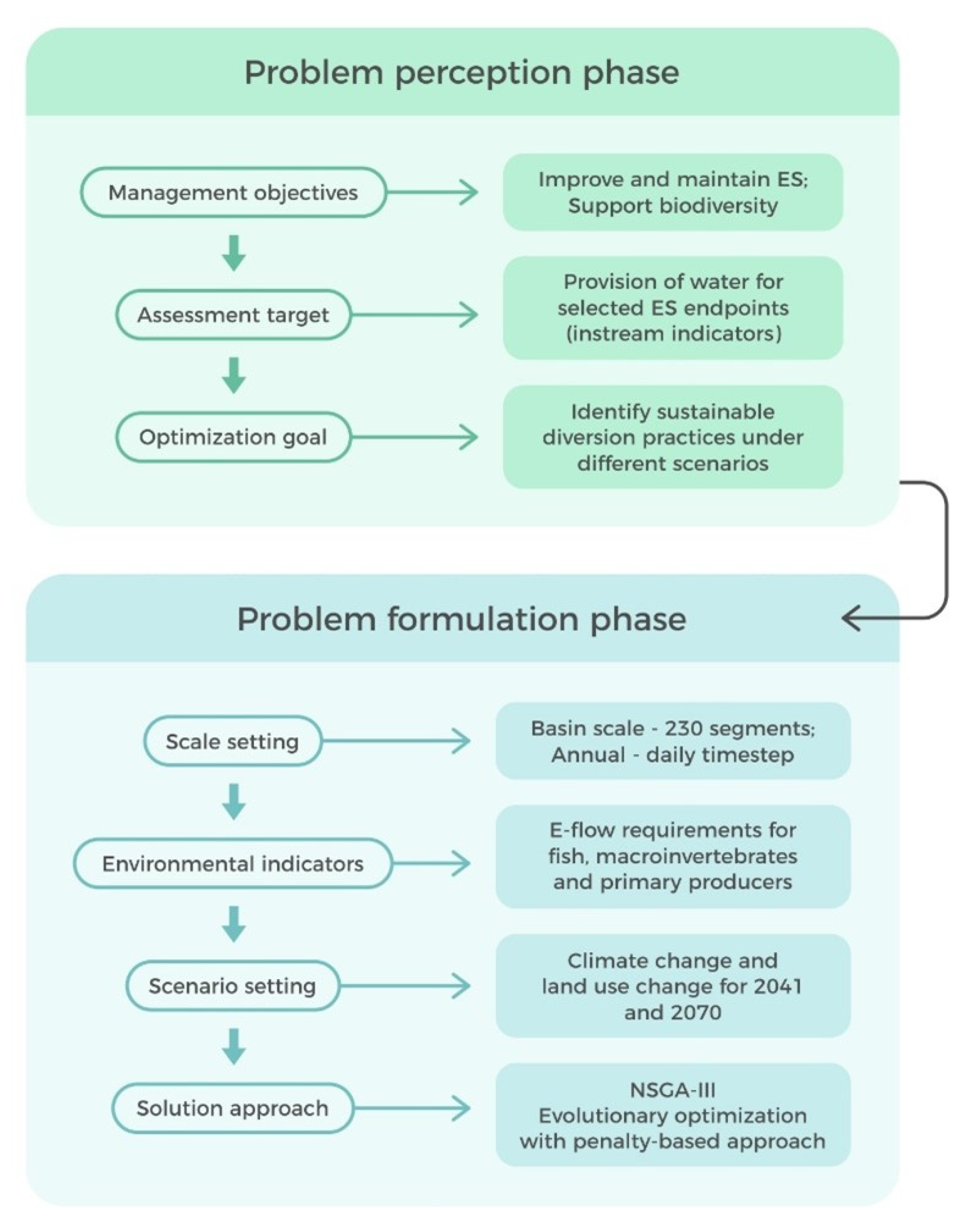
2.2. Problem Perception and Problem Formulation Phase for the Pas River Basin

An optimization assessment for water management typically starts with the identification and contextualization of a water management problem by defining objectives, targets, and goals [39], followed by the definition of the optimization model in terms of simulation assumptions and conditions [33,34]. These two phases can be described as the problem perception and problem formulation phases (see [33,40]), as illustrated in Figure 2. The two-step process is presented for the Pas River basin.

2.2.1. Problem Perception: Objectives and Optimization Goals

Contextualization helps to identify important values for river water management. Although a participatory approach can be used to contextualize the management problem [41], for simplicity, we formulated the overall management priorities for the Pas River basin as municipal water diversion planning to sustain ecosystem processes.
As part of the problem perception phase, we considered the improvement or maintenance of ES supporting the biodiversity in the Pas River basin while simultaneously providing sufficient water for the municipalities as the primary management-planning objective (Figure 2, top box). With this management objective in mind, we considered the provision of adequate instream hydrological conditions as an assessment target. Such conditions are the basis for setting the optimization goals to meet the ecohydrological requirements for key instream ES indicators (fish, macroinvertebrates, and primary producers; see Section “Environmental Indicators—Definition of Relevant Ecosystem Services for the Pas River”).

2.2.2. Problem Formulation

Based on the optimization goals identified in the problem perception phase, the problem formulation phase (Figure 2, bottom box) envisaged the following methodological steps. Regarding the modeling scale setting, the entire river basin network is considered to be the appropriate scale for both management and modeling. A spatial resolution of 500 m segments was set to allow local scale exploration on a daily time step within the year. The length choice was based on an existing Pas river network data layer. The next step consists of the processing of plausible environmental change scenarios (i.e., reference historical and future conditions of climate and land use) as a testing ground for the considered management planning objectives (i.e., optimization objectives) at two time points (2041 and 2070). In the following, the definition of expert-knowledge-based e-flow requirements (including the related timeframe) for key instream biological groups (fish, macroinvertebrates, and primary producers) underlying the Supporting ES indicators was carried out. Finally, an appropriate solution approach (i.e., evolutionary optimization) was chosen for the optimization problem to minimize the violations of the target hydrological metrics while maximizing the total water available for municipal consumption (see Section “Solution Approach to the Optimization Problem”).

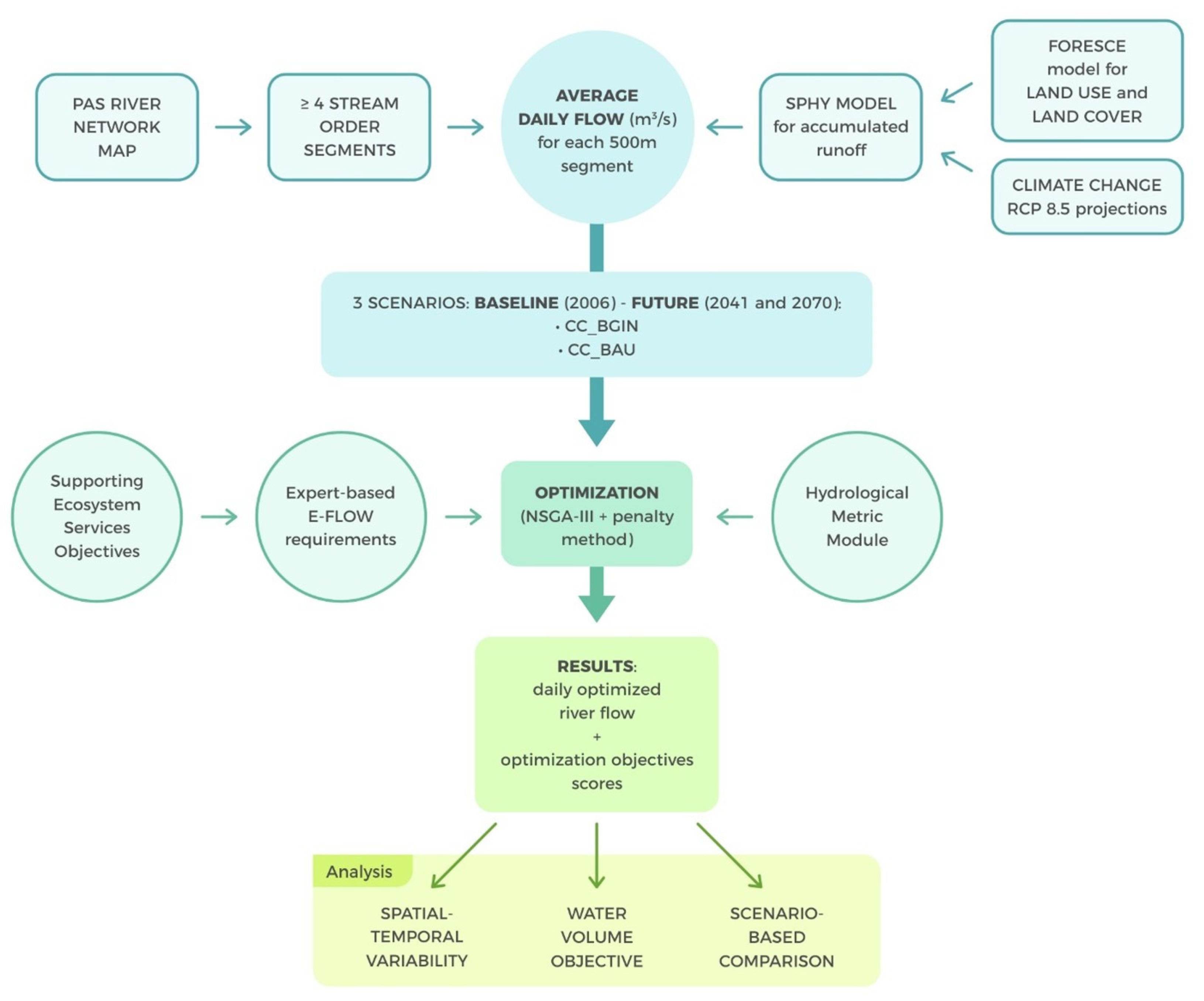
Scale and Scenario Setting

Land cover can change the magnitude and variability of instream flow attending to its influence on several runoff processes in the catchment [42,43,44,45]. Hence, different land cover and climate change scenarios can be used to simulate the resulting river runoff in the basin.
To capture changes in river runoff throughout space and time, we set the spatial scale of the assessment to the stream order ≥ 4 river network composed of 500 m long RS at the daily time step. The hydrological data used for optimization simulation were provided by the Instituto de Hidráulica Ambiental - Universidad de Cantabria (IHCantabria) and developed under the [46] for three environmental scenarios in the basin, considering historical (baseline) conditions and two plausible future conditions (Table 1). Figure 3 shows an overview flowchart of the main steps related to the problem formulation phase. The environmental scenarios accounted for land use (LU) and land cover (LC) changes and future climate change projections:
-
The LU and LC scenarios were developed using the process-based model framework FORE-SCE Model (Forecasting scenario for land change modeling) [47,48]. The FORE-SCE Model simulated current land use and cover by processing elevation, slope, and orientation and modeled fire recurrence. Furthermore, it models the influence of socioeconomic drivers obtained from interviews with local stakeholders and experts in agricultural and urban development policy fields. The input LU and LC maps were derived from historical remote sensing data (Landsat/Sentinel-2 imageries) for the 1990s, 2000s, and 2018 at a spatial resolution of 10 m.
-
For climate projections, historical data (from 1950 to 2018) and future data (from 2041 to 2070) on temperature and precipitation were used. See the procedure described in [49].
-
The final accumulated river surface runoff data (i.e., the resulting flow in the river) were produced by applying the distributed hydrological model SPHY (Spatial Processes in Hydrology; [50]) at a spatial resolution of 100 m and at the daily time step. Historical precipitation and temperature data for the period 1950 to 2018 were retrieved from the E-OBS v20e database [51] and resampled to produce a spatial resolution of ~1 km. [49] performed a statistical downscaling of precipitation and temperature with Ordinary Least Squares with yearly daily means using latitude, elevation, and Euclidean distance to the coastline as explanatory variables. For future scenarios, climatic datasets from a five-member ensemble of GCM-RCM chain simulations were retrieved for the development of climate change projections for the Pas catchment [49]. Further details of the procedure to develop climatic historical and future series can be found in [49]. Details of the model parameterization are provided in Table S1 in the Supplementary Materials. As shown in Table S2 in the Supplementary Materials, the results of the SPHY simulation (which are used by the optimization model) are characterized by a decline in precipitation and an increase in temperature and water demand due to land use changes. This, in turn, leads to a rise in actual evapotranspiration, causing a decrease in average instream flow in the Pas River basin, with a mean flow reduction rate of 25% between the basin outlets in the 1980–2012 and the 2041–2070 periods.
Table 1. Details of the scenarios considered in the optimization assessment for the Pas River basin.
Timeframe of
Source Data
Considered Period for ModelingScenario NameDescription
Historical1980–2012
  • 1/10/2005–30/9/2006
Present day (PR)This scenario represents present-day land cover and present-day climate. It is used as a comparison to the historical conditions.
Future2041–2070
  • 1/10/2041–30/9/2042
  • 1/10/2069–30/9/2070
BAU future (CC_BAU)This scenario assumes river discharge is affected by Business as Usual (BAU) future land cover and future climate (RCP 8.5; [49]. It considers the evolution of present-day land use and land cover conditions. In particular, forest patches (monoculture planted forest) development is implemented but not prioritized with the presence of shrubs and rushes. In the upper basin, there is a significant rural abandonment with forest recovery from pastureland, whereas the lower basin is characterized by urban area expansion and agricultural intensification.
Nature-based solutions prioritization (CC_BGIN)This scenario assumes an investment in nature-based solutions and an RCP 8.5 climate change intensity conditions [49]. Concerning the “future conditions” scenario, we have a modification of the rules for land use-land cover evolution (e.g., no fires and forest transitions are favored in places where it can have the highest impact on regulatory ES). This results in a prevalence of hill-side forests (e.g., oak, beech, chestnut, birch species) and riparian forests (e.g., willows, ash, alders).
To obtain the hydrological time series for the hydrological year, starting on 1 October and ending on 30 September, with a resolution of 500 m, each RS was linked to the nearest cell value of each scenario dataset (i.e., raster layer of simulated daily averaged accumulated surface runoff for the period 2041–2070). Two time points were considered for each scenario (i.e., 2041 and 2070) to explore the scenario-related simulation outputs of the water diversion planning objectives defined in Section “Solution Approach to the Optimization Problem”.
The choice of 31 years between the considered time points was intended to capture all possible changes in the basin based on the pre-set conditions to facilitate results comparison. Moreover, we believe this gap can be useful for management purposes. For reference, a hydrological series belonging to the year 2006 was extracted from the historical scenario and used as a present-day baseline. This particular year was chosen because it was the closest representation of a year with normal water conditions. For further insights into these results, we refer to the percent coverage distribution for the different land cover types under each scenario provided in Table S3 in the Supplementary Materials.

Environmental Indicators—Definition of Relevant Ecosystem Services for the Pas River

The ecosystem services (ES) concept emphasizes the significance of essential environmental assets and lends itself as an indicator of sustainable management strategies’ effectiveness at broader scales [52]. River ES supply is heavily reliant on the maintenance of in-stream conditions, as the ecological processes and functions are strongly connected to specific attributes of the flow regime [10,53]. As a result, in order to safeguard and preserve ES, hydrological conditions can be elicited to prioritize target ecological processes and functions and species requirements [9,10,11,13].
In this study, we defined three Supporting ES indicators by explicitly associating them with specific environmental flow (e-flow) requirements for key ecosystem components representing three levels of the river ecosystem food web. The Supporting ES category was chosen because the flow attributes underlying the supporting services can be easily related to the e-flow needed for habitats, life stages, and processes. Moreover, while there is a higher emphasis on Provisioning ES, as it provides the most evident benefit to society [9], Supporting ES can be a valuable indicator for river diversion management as it helps to define minimum standards for sustainable river water diversion.
We assumed that failure to meet the specified e-flow requirements would adversely affect the supply capacity of a specific Supporting ES. This simplification was essential since the optimization simulation we presented cannot quantify the reduction in the supply of Supporting ES and is not meant to explicitly account for synergies and linkages between different categories of ES. E-flows for key ecological components of the river ecosystem (fish, macroinvertebrates, and primary producers) were incorporated into the optimization assessment by considering distinct ecological endpoints as targets. Such ecological endpoints correspond with development stages (e.g., fish spawning) or taxonomic indicators (e.g., highest macroinvertebrate richness) connected to flow events or conditions in a specific time window throughout the hydrological year. We used a set of flow indices based on expert judgment as limiting conditions to diversion to represent hydrological thresholds for the selected ecological endpoints, reflecting Supporting ES supply. In other words, river flow optimized for diversion takes into account the hydrological conditions that must be met to sustain Supporting ES supply in the basin. More specifically, the Supporting ES considered were: Provision of habitat conditions for fish, Life-supporting conditions for macroinvertebrates, and Primary productivity. A description of the considered Supporting ES is shown in Table 2.
The definition of e-flow requirements underlying the Supporting ES indicators was obtained from [35]. However, to reflect more realistic conditions and in the light of novel evidence data, the hydrological and temporal thresholds were adjusted for this study. A summary of the e-flow requirements and thresholds used in this study is available in Table S4 in the Supplementary Materials. For a detailed description, please refer to [35].

Solution Approach to the Optimization Problem

Optimization models are computational tools that solve conflicting objectives, such as those related to water diversion management and planning in large river basins. Such conflicts often arise between the demands for river water to support the river ecosystem and for human use on the other side (for additional examples of water management conflicts, see [33]).
Before defining the technical features of the optimization model, we evaluated different solutions in the sense of a solution concept to better reflect the modeling needs and increase transparency in the model development process (sensu [33]). One solution to the problem follows a top-down approach, limiting the daily water demand (i.e., diversion) based on the annual water demand of all municipalities in the basin. The remaining daily river flow would be tested against the defined e-flow requirements. However, with this approach, it is more likely that ecosystem needs will not be met, and quantifying medium- to long-term needs is complex and adds to existing uncertainty. On the other hand, a bottom-up approach that matches e-flow requirements with available flow increases the chances of maintaining ES and, in a cross-scenario assessment, can identify diversion planning needs for environmental change adaptation. Hence, we decided to follow the latter approach.
Based on the selected Supporting ES and linked hydrological indicators, the optimization problem was characterized by four conflicting objectives (i.e., three for ES and one for the human supply). The human supply objective corresponds to the maximum amount of water that can be diverted from the river to meet human needs (i.e., municipal) as described in Sub-section S5 of Section B of the Supplementary Materials. The optimization model was set to maximize the flow (in m³/s) that can be diverted for human supply while minimizing the non-compliance of defined e-flow requirements underlying the three Supporting ES. A penalty-based solution approach was implemented to penalize e-flow objective functions when a violation of the specified constraints (i.e., constraints to the water flowing in the river and potentially available for diversion) was detected. In this way, we formulated an unconstrained optimization problem but considered certain conditions that had to be met to obtain solutions with minor violations. In the penalty method, which is integrated into the objective functions, each flow condition that is below the threshold is penalized by the algorithm based on the degree of the violation. Scaling between zero and one (i.e., best and worst result, respectively) is applied by normalizing the violation based on the individual constraint features. For a detailed explanation of unconstrained optimization and penalty methods, see [54,55]. The mathematical equations defining the optimization problem are presented in Section B of the Supplementary Materials.
Evolutionary optimization was used to solve such a non-linear optimization problem, following the approach of [35]. The optimization model was developed using the Pymoo (Multi-Objective Optimization in Python) framework version 0.4.1. [56] for the NSGA-III (Non-Dominated Sorting Genetic Algorithm III). The genetic algorithms (GA) at the base of the Pymoo optimization framework are very versatile, as they allow the simultaneous optimization of multiple objectives by imitating the process of natural selection of eliciting chromosomes throughout the search process [57]. The NSGA-III [58,59] provides a good chance of rapidly approximating a globally optimal solution. A hydrological metric module was run with the Pymoo optimization framework to calculate the hydrological indicators used for the e-flow requirements at each generation. An initial random population of “optimal” discharge volumes (in m3/s) is generated by the algorithm. The fitness of the residual discharge in the river (the difference between the scenario-based reference discharge in the river and the “optimal” discharge volume) is evaluated at each generation based on the degree of penalty violations for each optimization objective.
In the present study, the optimization model framework was run once for each independent RS within the considered time point and scenarios (i.e., five total model runs per scenario setup), generating unique results for each RS. The output of each model run was 230 optimal discharge volumes (i.e., one for each RS) for each scenario. The choice to run the optimization algorithm only once for each RS and scenario was based on the algorithm performance reported in the initial study by [35]. The study by [35] showed that a model set up envisaging 1000 generations (for 100 individuals) was appropriate for the convergence of the solution front to the ideal (i.e., its approximation). This was confirmed by a Running Metric Indicator [60] real-time measuring the objectives space from one generation to another that found similar patterns in the results from multiple simulations. The Running Metric is useful when termination criteria are not stated. An example of the convergence is given in Figure S1 of the Supplementary Materials. The final population of optimization scores was produced by implementing a preference-neutral approach by averaging the optimization objectives scores of the optimal population.

3. Results

3.1. Performance of the Optimization Objectives

As a first step in the analysis of the results, we evaluated the performance of the optimization objectives under the different scenarios, i.e., the total water volume available for consumption (i.e., municipal supply) while maintaining the prescribed diversion limits. The simulation results showed that the optimization objective (i.e., the total volume of river water in Hm3/y) can satisfy the water demand of the municipalities in the Pas River basin of the projected water demand for the year 2040 (i.e., around 7 Hm3/y) [61]. However, the water volumes differed significantly between the scenarios considered. While the baseline simulations (for the year 2006) predicted an average of 91.1 Hm³/y available for diversion, the future scenarios (for the year 2041) predicted 86.9 and 86.7 Hm³/y for the CC_BGIN and CC_BAU, respectively. For the same scenarios under future 2070 conditions, the model simulated 67.4 and 70.4 Hm³/y available for diversion. These results can be linked to the ability of the SPHY model to generate projected hydrological data to capture interactions between flow and land cover (e.g., the extent of forest cover vs. maturity).
On the other hand, the optimization results for the selected ES indicators along the river network (see Figures S2–S4 of the Supplementary Materials, Figure 4 shows results for Habitat condition provision for fish life-stages ES) showed the highest scores (i.e., least optimal results) for the provision of suitable habitat conditions for the different life stages of fish. This was observed in particular for the downstream river segments of the basin. At the same time, the highest heterogeneity of optimization scores was achieved in the upstream reaches in both the future BGIN_CC and BAU_CC scenarios. Optimization scores are absolute values that measure the conditions for achieving ES objectives. Values closest to zero represent the optimal conditions for ES for a given model simulation. While higher scores (>3.0) in the 2006 baseline scenario (PR) indicate existing hydrological pressure on the specific indicator, the reduction (scores between 0.9–1.6) in the optimization scores in the future scenarios increased the capacity of the river system to provide habitat conditions for fish. Conversely, a reverse pattern emerged for the ES indicator primary productivity, where the results showed the highest optimization scores in the upstream reaches. Interestingly, the macroinvertebrate objective was zero at each RS and scenario, indicating that the baseline and projected river flow could meet the defined instream conditions. However, this result may also be due to the type of hydrological indicator considered for the specific optimization objective. Furthermore, small inlets close to the downstream segments of the main river network were characterized by reduced optimized discharge with respect to the remaining river network due to their reduced discharge and variability.

3.2. Spatial and Temporal Distribution of Water Available for Diversion in the Pas River Basin

The second objective of the assessment was to evaluate the spatiotemporal distribution of water available for diversion in the Pas River basin after optimization. In the first step, we investigated the spatial distribution of the optimized daily river discharge available for diversion. The daily values of the river flow optimized for diversion in the Pas River basin can be accessed as an interactive map for each scenario at the following link: https://doi.org/10.6084/m9.figshare.19636449.v4 (accessed on 27 July 2023) [62]. The monthly averaged static maps of optimized instream flow for the baseline year (2006), and the 2041–2070 CC_BAU and CC_BGIN scenarios are available in Figures S5–S9 of the Supplementary Materials. Upstream river segments showed higher variation in the water volumes optimized for diversion than downstream segments. Upon comparison of the different scenarios, it is evident that the observed pattern remained consistent across all environmental conditions considered in the simulation. This consistency could be attributed to the chosen hydrological indicator (i.e., cumulative runoff for each segment of the river) and the anticipated increase in flow magnitude as the river network approached its outlets. Lastly, we analyzed the simulation results by reviewing the seasonal river discharge averages to explore which time scales were particularly relevant for management and policy. Figure 5 depicts these findings. The results showed a decrease in the average optimized discharge for the fall season for both scenarios in 2070. However, a slightly higher average optimized discharge was observed for the spring and summer seasons. In all future scenarios (2041–2070), there was a decrease in the average flow available for diversion during winter. Although there were minor differences in the overall trends between the BGIN_CC and BAU_CC scenarios, the variations were not significant.

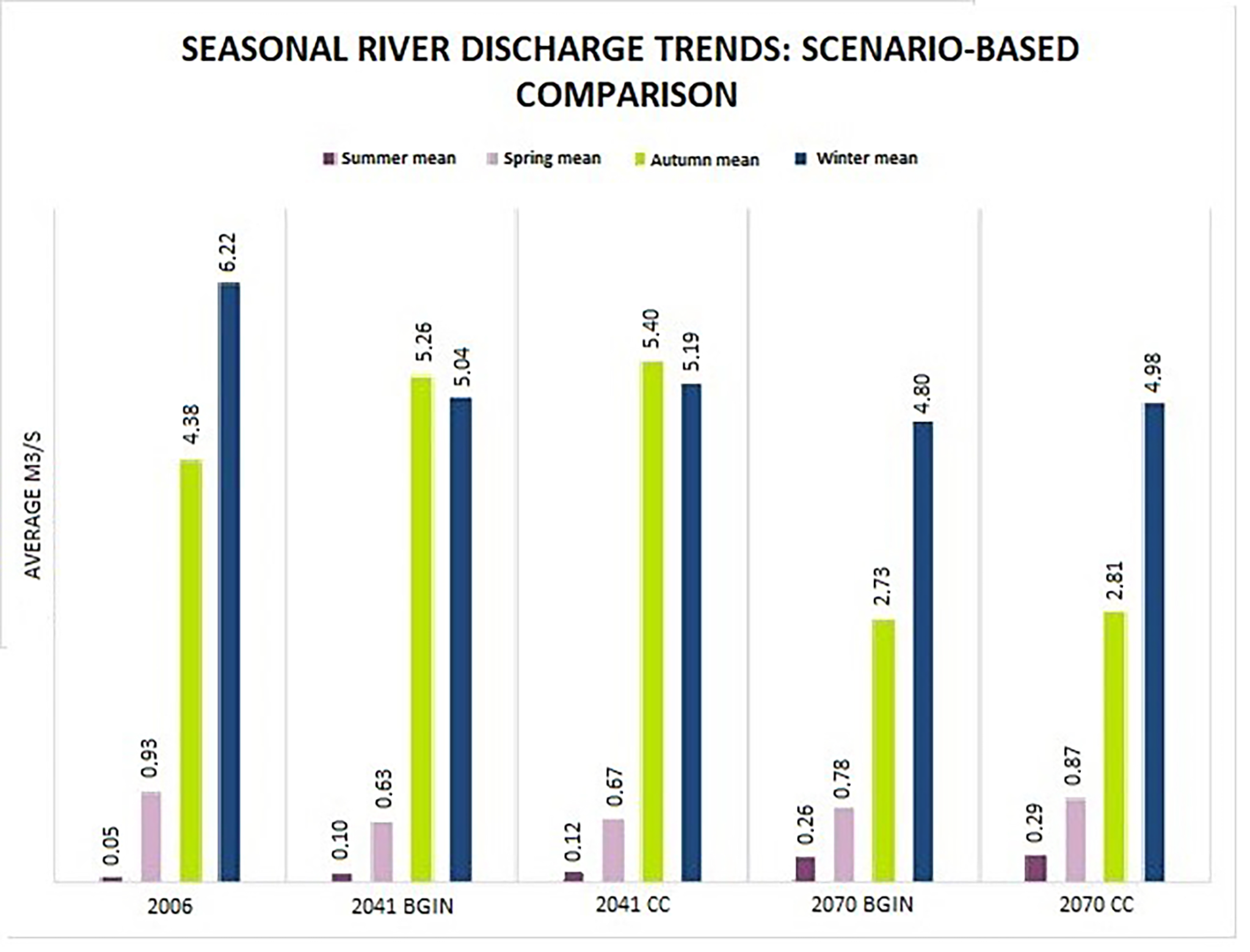
3.3. Comparison of Results within the Different Scenarios

To understand the rate of variability in average discharge values throughout the year, we processed the results as a frequency distribution of average discharge values under each scenario. An illustration of this for the baseline scenario can be found in Figure 6. Additional findings are available in Figures S10–S13 in the Supplementary Materials). The results show that the most significant variability in optimized average discharge values throughout the basin is likely to occur from December to March, whereas the period spanning May to October proved to be the most stable.
Due to the amount of data generated, four RS were selected to illustrate in detail the results of different locations along the river network and to analyze the results at different locations in the river network (see Figure S10 in the Supplementary Materials). To examine the interannual trends, we plotted the natural flow against the flow resulting from the optimization simulation and available for abstraction for the four representative RS (Figure 7 and Figure S14); see “A-B-C-D” in Figure 8 as an example for the BGIN_CC scenario of the year 2041 (other results are available in Figures S15–S18 of the Supplementary Materials). The comparison of the natural flow and the optimized flow for diversion between scenarios shows that for most of the year, a sufficient portion of the river flow is available for diversion (i.e., the optimized flow mainly follows the natural flow regime), demonstrating a reduced trade-off between objectives (i.e., municipal supply and ecosystem services). However, during the driest periods of the year, a larger proportion of the flow is needed to maintain and meet ecological thresholds. Notably, in the 2041 scenarios, the model identified a lower optimal discharge during the dry months despite a prominent natural flow, indicating a greater trade-off based on ecological needs and defined requirements.

4. Discussion

4.1. Spatial and Temporal Scale Considerations of Water Available for Diversion

Knowledge of the future spatial and temporal variability of water available for consumptive needs (e.g., drinking water) provides an advantage for water diversion management that aims at reducing uncertainty in management outcomes. Although it is not possible to provide absolute results (because we cannot reduce all potential sources of uncertainty; [31,63]), evaluating objectives under a range of scenarios can help identify appropriate management strategies in the present to achieve long-term diversion goals. From a spatial perspective, typically most basin management strategies focus on the entire network or significant parts to achieve specific downstream abstraction objectives [64]. Our results showed that while river water optimized for diversion can meet annual municipal water supply under all scenarios, the average daily and monthly optimized flow can vary significantly at different locations in the river network, which poses a challenge for maintaining adequate conditions for ES throughout the year and providing supply during dry periods. To address this, diversion management can define site-specific water supply targets and support the ecosystems’ hydrological needs. Furthermore, river and land management planning could consider relocating abstraction-dependent facilities downstream where discharge is more stable. From the temporal perspective, our study has found that downstream river segments maintain a more stable optimized discharge throughout the year compared to upstream river segments, which experience greater variability. This pattern was observed across all scenarios and can be attributed to the higher sensitivity of upstream reaches to climate events. However, more research is needed to evaluate the influence of land cover and instream flow in these areas. Although these results are related to our case study, they underline the importance of analyzing temporal hydrological patterns across the entire river network.
Our study suggests that the main challenges for basin management under the scenarios considered are related to the pronounced seasonal differences in optimized discharge at each river segment, leading to spatial heterogeneity across the network. Incorporating these spatial and temporal aspects into management planning, for example, by distinguishing between river segments that exhibit the greatest variation in streamflow over the year, would help reduce the risk of major trade-offs in river water allocation in future diversion programs and promote the implementation of adaptive management.

4.2. Supporting Ecosystem Services Objectives across Scenarios

Our study assessed the future sustainability of diversion decisions by examining optimization scores change between time points in the short and medium term (i.e., 2041 and 2070) and scenarios at each river segment. In regulated basins, maintaining conditions for fish is typically a critical water management objective because of their intrinsic value and connection to other ES supply (e.g., fisheries, recreational) [8]. Fish species require a range of specific hydrological conditions for each life stage. The ES objective ‘provision habitat conditions for fish life stages’ showed high optimization scores (i.e., least optimal result) in the downstream reaches in the baseline scenario. These scores decreased in both CC_BGIN and CC_BAU scenarios, with slight additional improvement (i.e., slightly lower scores) for the year 2070. While downstream reaches are usually characterized by more stable discharge, this result could be related to the simulation conditions. However, it is crucial to take into account the influence of severe occurrences on hydrological behavior. Such events might have disturbed the timely flows of freshwater and peak flows, resulting in affecting the model’s fish requirements. Conversely, the ES of ‘primary productivity’ required stable low-flow minimum conditions throughout determined periods in the year, resulting in a higher score for upstream reaches in both scenarios and time points. This indicates that water-diversion-planning trade-offs involve the priority of supplying low flows upstream of the river network while ensuring that peak flows downstream are maintained. Other studies also found that upstream water abstraction impairs downstream ecological functions and can expose the basin to water scarcity [65]. On the one hand, our results confirm that even enough natural discharge downstream of the river is not sufficient to ensure the achievement of optimal scores for all ES objectives considered. However, this could also be related to the differences in the formulation of the equations at the base of the optimization objectives (e.g., the indicators chosen). A possible solution could be distinguishing areas where ES are generated and consumed, as suggested by the study of [9]. This can likely reduce this bias by regarding only locations where Supporting ES are generated.
The Supporting ES objectives scores showed significant variability in their specific supply capacity (Provision of habitat conditions for fish ES, Life-supporting conditions for macroinvertebrates ES, Primary Productivity ES) throughout the network, while the comparison of the scenarios (CC_BAU and CC_BGIN) did not show any noticeable difference. Instead, trade-offs were found to be inherent in the spatial and temporal dimensions of diversion planning. Thus, the failure to recognize the spatial variability of discharge conditions for each RS under consideration may result in overlooking hotspots of reduced supply that must be investigated to achieve long-term management objectives. While the results of implementing such goals need to be monitored to verify their durability in the real world, the results of our study showed that, overall, the considered e-flow requirements (i.e., hydrological indices associated with ecological processes) can provide a good compromise for diversion water management needs to ensure sufficient river water for key ecosystem endpoints and municipal needs.

4.3. Optimization Set-Up and Scenarios for Water Diversion Management at Different Scales

Defining a set of plausible conditions under which the model will “operate” or be tested is the second step after defining the model. In optimization, this usually corresponds to establishing rules and objectives and then running the model for specific input conditions (e.g., hydrological, climatic, and LU and LC patterns) [33,34]. The input conditions can be calibrated based on projected changes in environmental drivers (i.e., scenarios) that could affect the system. Critical drivers of change in river basins (and the water they provide) include, in particular, land use and climate change [66,67,68], which introduce a large degree of uncertainty in the results obtained. While uncertainty can be treated in different ways in optimization modeling, [69] points out that “decision-makers are not particularly interested in uncertainty per se […]. Rather, they are interested in knowing whether particular decision strategies are robust across a range of possibilities”. This range of possibilities can be more or less roughly represented by scenarios, which can be used to identify management plans and strategies independent of future conditions [63].
Based on our explorative research and acknowledging the results from [35], optimizing environmental change scenarios (i.e., input hydrological conditions, in the case of optimization applied for diversion) at large scales such as river basins and sub-basins can lead to more effective identification of patterns of spatial-temporal changes in water availability for diversion to prioritize hotspots for shortages. On the other hand, once hotspots have been identified, river-segment-specific hydrological features can be tested by modifying optimization constraints (i.e., limiting conditions), for example, by relating hydrological patterns to the response of adjacent habitats, species requirements, and landscape features (e.g., mountains slopes). However, both assessment scales would benefit from good-quality input data and assumptions about system processes (i.e., knowledge of how the system behaves). While the former can be controlled to some extent through careful selection and pre-processing, the latter will always be affected by some degree of uncertainty (i.e., aleatory uncertainty as opposed to epistemic uncertainty; [40,63]) which cannot be eliminated. Another solution to reduce uncertainty is to run the model multiple times. However, this would significantly increase the computational effort and long post-processing times, especially for large river basins. We acknowledge that simplified assumptions about future climate and environmental system states and a few model runs have been made in this study. In addition, the inclusion of an optimization module to take into account the cumulative impact of diverting river water from upstream river segments on the downstream discharge would allow an improved assessment of river flow available for diversion. Therefore, while the exploratory assessment has some limitations that can be addressed in future applications, our modeling application can still provide a simple means for examining the implications of water diversion management decisions by incorporating segment-level information. It is worth noting that the results do not offer an exact representation of the optimized daily flow behavior for each scenario but rather should be used to derive the uncertainty space for implementing future water availability for diversion. To make informed decisions for adaptation of management programs to future conditions (i.e., through informed decisions), it is vital to have a broader view of detailed river flow information such as river segment data at basin scales. Assessing water diversion at small scales provides limited information to managers and reduces their ability to take effective action when changes occur [70].

4.4. Considerations on Optimization Indicators for Ecological Endpoints

To effectively manage the impact of river water diversion on instream ecosystems, it is crucial to identify the hydrological conditions that are necessary to support ecological endpoints. The literature provides many examples of hydrological conditions linked to specific ecosystem components (especially biological groups or species) through e-flows (the magnitude, timing, and rate of change), which can be linked to indicators for supporting ES. Regardless of which concept better fits the management needs of the particular case study, to define ecological instream flow requirements for optimization modeling, we recommend taking the following considerations based on our study: (1) Focusing solely on keystone species or relevant ecosystem components in the basin is convenient for optimization, as it can capture the most critical hydrological components, but it may miss other important hydrological processes. In this case, the choice is either to justify the selection of a limited number of ecosystem components or to expand the range of hydrological processes considered in the optimization model, which would require more modeling efforts. (2) Our study results show that optimization scores for supporting ES objectives are unevenly distributed across the basin and scenarios. This suggests that while the scenarios help test the appropriateness of overall management objectives in light of future changes, more insight can be gained by targeting locally tailored ecological objectives. For example, prioritizing some ecosystem components and their hydrological requirements downstream of the river network while focusing on others upstream. (3) Consider the possibility of ecological process adaptation. More specifically, if the time horizon considers long-term management objectives, it should be recognized that some species adaptation may have occurred by the end of the planned management period while management outcomes are manifested. The failure to account for potential ecosystem adaptations when applying optimization models can skew the assessments and render results useless. Although this may be one of the most challenging tasks for modern water management, many recommendations have already been made in the current literature to account for these changes [71]. However, more precise information is needed this can be achieved with optimization.

5. Recommendations

Based on the results of the exploratory optimization assessment conducted in this study, a series of recommendations were formulated for both water managers and water management analysts/modelers. These recommendations aim to facilitate basin-scale diversion management planning and enable the adoption of an adaptive management approach (see Table 3).

6. Conclusions

This study considered the Pas River basin as a test site to examine the spatial and temporal implications of river water diversions. The objective of the optimization assessment was to identify future challenges for diversion planning, taking into account the hydrological requirements for key instream supporting ecosystem services and the annual municipal water demand. Two future environmental change (land use, climate) scenarios were considered. While the daily river water available for diversion was found to meet municipal needs under the considered scenarios, the study results showed that seasonal shifts and spatial heterogeneity in diversion volumes and the optimal provision of ecosystem services represent the most significant challenges for medium- to long-term diversion management. Based on our findings, we provided considerations and recommendations for organizing river water diversion management efforts at the basin scale to achieve an adaptive approach. Diversion planning should consider the seasonal time frame for setting diversion targets and consider site-specific ecological goals that maintain the provision of supporting ecosystem services.
While the assessment presented in this study can assist in pinpointing viable diversion locations and strategizing withdrawal timing, forthcoming investigative analyses using optimization should incorporate the effects of severe climate change events and insights from enhanced land cover-hydrology modeling. This entails taking into account the holistic influence of land cover in a given region on river discharge at a designated site and the maturity of local forests. Moreover, conducting several simulations can help mitigate any uncertainties related to data in subsequent practical applications.

Supplementary Materials

The following supporting information can be downloaded at: https://www.mdpi.com/article/10.3390/w15183289/s1, Section A, Table S1: SPHY model (see Section “Scale and scenario setting”) input type and their values for the generation of the surface runoff for the river network in the considered case study area; Table S2: Variation of the environmental parameters for the present (1980–2012) and future (2041–2070) time periods considered in the study; Table S3: Percentage cover for each class and each scenario considered in the optimization simulation; Table S4: Summary of the e-flow requirements (EFR) considered in the study. The EFR define the hydrological conditions to be conserved in the river during the daily diversion operations throughout the year. The table shows the duration, the hydrological metric used, and the month of the year relevant for each EFR. Legend: %MMF = percentage value of mean monthly flow; Qm7 = 7 times the median annual flow; Q75 = the flow value that is exceeded 25% of the time; %MYF = percentage value of the mean yearly flow; Section B, Figure S1: The Running Metric Indicator (Blank and Deb, 2020) for a test RS simulation. The ∆f indicator measures the convergence of the objective space at each generation. Section C, Figure S2: Maps showing the spatial distribution of the optimization objective scores for the Habitat condition provision for fish life-stages ES under each considered scenario; Figure S3: Maps showing the spatial distribution of the optimization objective scores for the life-supporting conditions for Macroinvertebrate taxa richness ES under each considered scenario; Figure S4: Maps showing the spatial distribution of the optimization objective scores for the Primary productivity ES under each considered scenario; Figure S5: Monthly averaged optimized instream flow for the PR scenario (2006); Figure S6: Monthly averaged optimized instream flow for the CC_BAU 2041 scenario; Figure S7: Monthly averaged optimized instream flow for the CC_BGIN 2041 scenario; Figure S8: Monthly averaged optimized instream flow for the CC_BGIN 2070 scenario; Figure S9: Monthly averaged optimized instream flow for the CC_BAU 2070 scenario; Figure S10: Heatmap showing the average optimized discharge (in m3/s) value (on the x-axis) for each month (on the y-axis) for the 2041 BGIN_CC scenario; Figure S11: Heatmap showing the average optimized discharge (in m3/s) value (on the x-axis) for each month (on the y-axis) for the 2041 BAU_CC scenario; Figure S12: Heatmap showing the average optimized discharge (in m3/s) value (on the x-axis) for each month (on the y-axis) for the 2070 BGIN_CC scenario; Figure S13: Heatmap showing the average optimized discharge (in m3/s) value (on the x-axis) for each month (on the y-axis) for the 2070 BAU_CC scenario; Figure S14: Location of the representative points in the basin elicited for results presentation and discussion; Figures S15 and S16: Flow series showing the daily profile of the discharge (in m3/s) optimized for diversion (light blue thin line) plotted with respect to the river natural discharge (purple background shape) for the each of the four RS locations analyzed under the Baseline 2006 (PR) scenario (top) and 2041 BAU_CC scenario (bottom); Figures S17 and S18: Flow series showing the daily profile of the discharge (in m3/s) optimized for diversion (light blue thin line) plotted with respect to the river natural discharge (purple background shape) for the each of the four RS locations analyzed under the 2070 BGIN_CC (top) and 2070 BAU_CC scenario (bottom).

Author Contributions

Conceptualization, D.D. and M.V.; Methodology, D.D.; Formal Analysis, D.D.; Resources, F.J.P. and J.B.; Data Curation, D.D.; Writing—Original Draft Preparation, D.D.; Writing—Review and Editing; D.D., M.V., F.W., F.J.P. and J.B.; Visualization, D.D.; Supervision, M.V. and F.W. All authors have read and agreed to the published version of the manuscript.

Funding

This paper was an output of the Euro-FLOW project and received funding from the European Union’s Horizon 2020 Research and Innovation Programme under the Marie Skłodowska-Curie grant, agreement no. 765553. This publication is also part of the I+D+I project RIFFLE PID2020-114427RJ-I00 funded by MCIN/AEI/10.13039/501100011033.

Data Availability Statement

Input scenario-based hydrological data: Restrictions apply to the availability of these data. Data were obtained from IHCantabria and are available on request with the permission of IHCantabria. Python code: The code employed in this study is available on request from the corresponding author. This restriction is applied because part of the code was not developed by the authors.

Acknowledgments

We would like to thank Avril Horne from the University of Melbourne (Australia) for her valuable input during the early stages of paper development.

Conflicts of Interest

The authors declare no conflict of interest.

References

  1. Poff, N.; Allan, J.D.; Bain, M.; Karr, J.; Prestegaard, K.; Richter, B.; Sparks, R.; Stromberg, J. The Natural Flow Regime: A Paradigm for River Conservation and Restoration. Bioscience 1997, 47, 769–784. [Google Scholar] [CrossRef]
  2. Alamanos, A.; Koundouri, P. Emerging Challenges and the Future of Water Resources Management. HydroLink 2023, 4, 116–120. [Google Scholar]
  3. Grison, C.; Koop, S.; Eisenreich, S.; Hofman, J.; Chang, I.-S.; Wu, J.; Savic, D.; van Leeuwen, K. Integrated Water Resources Management in Cities in the World: Global Challenges. Water Resour. Manag. 2023, 37, 2787–2803. [Google Scholar] [CrossRef]
  4. Moghim, S.; Teuling, A.J.; Uijlenhoet, R. A Probabilistic Climate Change Assessment for Europe. Int. J. Climatol. 2022, 42, 6699–6715. [Google Scholar] [CrossRef]
  5. Ziolkowska, J.R.; Ziolkowski, B. Effectiveness of Water Management in Europe in the 21st Century. Water Resour. Manag. 2016, 30, 2261–2274. [Google Scholar] [CrossRef]
  6. Stewardson, M.J.; Acreman, M.; Costelloe, J.F.; Fletcher, T.D.; Fowler, K.J.A.; Horne, A.C.; Liu, G.; McClain, M.E.; Peel, M.C. Understanding Hydrological Alteration. In Water for the Environment: From Policy and Science to Implementation and Management; Elsevier Inc.: Amsterdam, The Netherlands, 2017; pp. 37–64. ISBN 9780128039458. [Google Scholar]
  7. Rolls, R.J.; Bond, N.R. Environmental and Ecological Effects of Flow Alteration in Surface Water Ecosystems. In Water for the Environment: From Policy and Science to Implementation and Management; Elsevier Inc.: Amsterdam, The Netherlands, 2017; pp. 65–82. ISBN 9780128039458. [Google Scholar]
  8. Watz, J.; Aldvén, D.; Andreasson, P.; Aziz, K.; Blixt, M.; Calles, O.; Lund Bjørnås, K.; Olsson, I.; Österling, M.; Stålhammar, S.; et al. Atlantic Salmon in Regulated Rivers: Understanding River Management through the Ecosystem Services Lens. Fish Fish. 2022, 23, 478–491. [Google Scholar] [CrossRef]
  9. Alan Yeakley, J.; Ervin, D.; Chang, H.; Granek, E.F.; Dujon, V.; Shandas, V.; Brown, D. Ecosystem Services of Streams and Rivers. In River Science; John Wiley & Sons, Ltd.: Chichester, UK, 2016; pp. 335–352. [Google Scholar]
  10. Gilvear, D.J.; Beevers, L.C.; O’Keeffe, J.; Acreman, M. Environmental Water Regimes and Natural Capital. In Water for the Environment; Horne, A.C., Webb, J.A., Stewardson, M.J., Richter, B., Acreman, M., Eds.; Elsevier: Amsterdam, The Netherlands, 2017; pp. 151–171. [Google Scholar]
  11. Jähnig, S.C.; Carolli, M.; Dehnhardt, A.; Jardine, T.; Podschun, S.; Pusch, M.; Scholz, M.; Tharme, R.E.; Wantzen, K.M.; Langhans, S.D. Ecosystem Services of River Systems—Irreplaceable, Undervalued, and at Risk. In Encyclopedia of Inland Waters; Elsevier: Amsterdam, The Netherlands, 2022; pp. 424–435. [Google Scholar]
  12. Rosero-López, D.; Knighton, J.; Lloret, P.; Encalada, A.C. Invertebrate Response to Impacts of Water Diversion and Flow Regulation in High-altitude Tropical Streams. River Res. Appl. 2020, 36, 223–233. [Google Scholar] [CrossRef]
  13. Ferreira, V.; Albariño, R.; Larrañaga, A.; LeRoy, C.J.; Masese, F.O.; Moretti, M.S. Ecosystem Services Provided by Small Streams: An Overview. Hydrobiologia 2022, 850, 2501–2535. [Google Scholar] [CrossRef]
  14. Arthington, A.H. Environmental Flows; University of California Press: Berkeley, CA, USA, 2012; ISBN 9780520273696. [Google Scholar]
  15. Fowler, K.; Peel, M.; Saft, M.; Nathan, R.; Horne, A.; Wilby, R.; McCutcheon, C.; Peterson, T. Hydrological Shifts Threaten Water Resources. Water Resour Res. 2022, 58, e2021WR031210. [Google Scholar] [CrossRef]
  16. Horne, A.C.; Webb, J.A.; Mussehl, M.; John, A.; Rumpff, L.; Fowler, K.; Lovell, D.; Poff, L.R. Not Just Another Assessment Method: Reimagining Environmental Flows Assessments in the Face of Uncertainty. Front Environ. Sci 2022, 10, 808943. [Google Scholar] [CrossRef]
  17. John, A.; Nathan, R.; Horne, A.; Stewardson, M.; Angus Webb, J. How to Incorporate Climate Change into Modelling Environmental Water Outcomes: A Review. J. Water Clim. Change 2020, 11, 327–340. [Google Scholar] [CrossRef]
  18. Judd, M.; Bond, N.; Horne, A.C. The Challenge of Setting “Climate Ready” Ecological Targets for Environmental Flow Planning. Front Environ. Sci. 2022, 10, 21. [Google Scholar] [CrossRef]
  19. Lowe, L.; Szemis, J.; Webb, J.A. Uncertainty and Environmental Water. In Water for the Environment: From Policy and Science to Implementation and Management; Elsevier Inc.: Amsterdam, The Netherlands, 2017; pp. 317–344. ISBN 9780128039458. [Google Scholar]
  20. Delavari Edalat, F.; Abdi, M.R. Adaptive Water Management; International Series in Operations Research & Management Science; Springer International Publishing: Cham, Germany, 2018; Volume 258, ISBN 978-3-319-64142-3. [Google Scholar]
  21. Pahl-Wostl, C.; Kabat, P.; Möltgen, J. Adaptive and Integrated Water Management: Coping with Complexity and Uncertainty; Springer: Berlin/Heidelberg, Germany, 2008; ISBN 9783540759409. [Google Scholar]
  22. Allan, C.; Watts, R.J. Revealing Adaptive Management of Environmental Flows. Environ. Manag. 2018, 61, 520–533. [Google Scholar] [CrossRef] [PubMed]
  23. Pahl-Wostl, C.; Lebel, L.; Knieper, C.; Nikitina, E. From Applying Panaceas to Mastering Complexity: Toward Adaptive Water Governance in River Basins. Environ. Sci. Policy 2012, 23, 24–34. [Google Scholar] [CrossRef]
  24. Sendzimir, J.; Jeffrey, P.; Aerts, J.; Berkamp, G.; Cross, K.; Pahl-Wostl, C.; Sendzimir, J.; Jeffrey, P.; Aerts, J.; Berkamp, G.; et al. Research, Part of a Special Feature on New Methods for Adaptive Water Management Managing Change toward Adaptive Water Management through Social Learning. Ecol. Soc. 2007, 12, 30. [Google Scholar]
  25. Webb, J.A.; Watts, R.J.; Allan, C.; Warner, A.T. Principles for Monitoring, Evaluation, and Adaptive Management of Environmental Water Regimes. In Water for the Environment: From Policy and Science to Implementation and Management; Elsevier Inc.: Amsterdam, The Netherlands, 2017; pp. 599–623. ISBN 9780128039458. [Google Scholar]
  26. Allan, C.; Curtis, A. Nipped in the Bud: Why Regional Scale Adaptive Management Is Not Blooming. Env. Manag. 2005, 36, 414–425. [Google Scholar] [CrossRef]
  27. Pahl-Wostl, C. Transitions towards Adaptive Management of Water Facing Climate and Global Change. Proc. Water Resour. Manag. 2007, 21, 49–62. [Google Scholar] [CrossRef]
  28. Badham, J.; Elsawah, S.; Guillaume, J.H.A.; Hamilton, S.H.; Hunt, R.J.; Jakeman, A.J.; Pierce, S.A.; Snow, V.O.; Babbar-Sebens, M.; Fu, B.; et al. Effective Modeling for Integrated Water Resource Management: A Guide to Contextual Practices by Phases and Steps and Future Opportunities. Environ. Model. Softw. 2019, 116, 40–56. [Google Scholar] [CrossRef]
  29. Borgomeo, E. Water Resource System Modelling for Climate Adaptation. In Proceedings of the Climate Adaptation Modelling; Kondrup, C., Mercogliano, P., Bosello, F., Mysiak, J., Scoccimarro, E., Rizzo, A., Ebrey, R., Ruiter, M.d., Jeuken, A., Watkiss, P., Eds.; Springer International Publishing: Cham, Germany, 2022; pp. 141–147. [Google Scholar]
  30. Candido, L.A.; Coêlho, G.A.G.; de Moraes, M.M.G.A.; Florêncio, L. Review of Decision Support Systems and Allocation Models for Integrated Water Resources Management Focusing on Joint Water Quantity-Quality. J. Water Resour. Plan Manag. 2022, 148, 03121001. [Google Scholar] [CrossRef]
  31. Kirchner, M.; Mitter, H.; Schneider, U.A.; Sommer, M.; Falkner, K.; Schmid, E. Uncertainty Concepts for Integrated Modeling—Review and Application for Identifying Uncertainties and Uncertainty Propagation Pathways. Environ. Model. Softw. 2021, 135, 104905. [Google Scholar] [CrossRef]
  32. Refsgaard, J.C.; van der Sluijs, J.P.; Højberg, A.L.; Vanrolleghem, P.A. Uncertainty in the Environmental Modelling Process—A Framework and Guidance. Environ. Model. Softw. 2007, 22, 1543–1556. [Google Scholar] [CrossRef]
  33. Derepasko, D.; Guillaume, J.H.A.; Horne, A.C.; Volk, M. Considering Scale within Optimization Procedures for Water Management Decisions: Balancing Environmental Flows and Human Needs. Environ. Model. Softw. 2021, 139, 104991. [Google Scholar] [CrossRef]
  34. Horne, A.; Szemis, J.M.; Kaur, S.; Webb, J.A.; Stewardson, M.J.; Costa, A.; Boland, N. Optimization Tools for Environmental Water Decisions: A Review of Strengths, Weaknesses, and Opportunities to Improve Adoption. Environ. Model. Softw. 2016, 84, 326–338. [Google Scholar] [CrossRef]
  35. Derepasko, D.; Peñas, F.J.; Barquín, J.; Volk, M. Applying Optimization to Support Adaptive Water Management of Rivers. Water 2021, 13, 1281. [Google Scholar] [CrossRef]
  36. Witing, F.; Forio, M.A.E.; Burdon, F.J.; Mckie, B.; Goethals, P.; Strauch, M.; Volk, M. Riparian Reforestation on the Landscape Scale: Navigating Trade-offs among Agricultural Production, Ecosystem Functioning and Biodiversity. J. Appl. Ecol. 2022, 59, 1456–1471. [Google Scholar] [CrossRef]
  37. Pérez Silos, I. Hacia Una Gestión Dinámica e Integral Del Paisaje En Cuencas de Montaña: Definición de Una Estrategia Adaptativa a Los Retos Derivados Del Cambio Global; Universidad de Cantabria: Santander, Spain, 2022. [Google Scholar]
  38. Belmar, O.; Barquín, J.; Álvarez-Martínez, J.M.; Peñas, F.J.; Del Jesus, M. The Role of Forest Maturity in Extreme Hydrological Events. Ecohydrology 2018, 11, e1947. [Google Scholar] [CrossRef]
  39. Horne, A.C.; Konrad, C.; Webb, J.A.; Acreman, M. Visions, Objectives, Targets, and Goals. In Water for the Environment: From Policy and Science to Implementation and Management; Elsevier Inc.: Amsterdam, The Netherlands, 2017; pp. 189–199. ISBN 9780128039458. [Google Scholar]
  40. Maier, H.R.; Kapelan, Z.; Kasprzyk, J.; Kollat, J.; Matott, L.S.; Cunha, M.C.; Dandy, G.C.; Gibbs, M.S.; Keedwell, E.; Marchi, A.; et al. Evolutionary Algorithms and Other Metaheuristics in Water Resources: Current Status, Research Challenges and Future Directions. Environ. Model. Softw. 2014, 62, 271–299. [Google Scholar] [CrossRef]
  41. Pahl-Wostl, C.; Mostert, E.; Tàbara, D. The Growing Importance of Social Learning in Water Resources Management and Sustainability Science. Ecol. Soc. 2008, 13, 24. [Google Scholar] [CrossRef]
  42. Kumar, M.; Denis, D.M.; Kundu, A.; Joshi, N.; Suryavanshi, S. Understanding Land Use/Land Cover and Climate Change Impacts on Hydrological Components of Usri Watershed, India. Appl. Water Sci. 2022, 12, 39. [Google Scholar] [CrossRef]
  43. Zeiger, S.; Hubbart, J. Assessing Environmental Flow Targets Using Pre-Settlement Land Cover: A SWAT Modeling Application. Water 2018, 10, 791. [Google Scholar] [CrossRef]
  44. Sampurno Bruijnzeel, L.A. Land Use and Landcover Effects on Runoff Processes: Forest Harvesting and Road Construction. In Encyclopedia of Hydrological Sciences; John Wiley & Sons, Ltd: Chichester, UK, 2005. [Google Scholar]
  45. Qazi, N.Q.; Bruijnzeel, L.A.; Rai, S.P.; Ghimire, C.P. Impact of Forest Degradation on Streamflow Regime and Runoff Response to Rainfall in the Garhwal Himalaya, Northwest India. Hydrol. Sci. J. 2017, 62, 1114–1130. [Google Scholar] [CrossRef]
  46. The ALICE Project. Available online: https://www.project-alice.com (accessed on 21 July 2023).
  47. Sohl, T.L.; Sayler, K.L.; Drummond, M.A.; Loveland, T.R. The FORE-SCE Model: A Practical Approach for Projecting Land Cover Change Using Scenario-Based Modeling. J. Land Use Sci. 2007, 2, 103–126. [Google Scholar] [CrossRef]
  48. Sohl, T.; Sayler, K. Using the FORE-SCE Model to Project Land-Cover Change in the Southeastern United States. Ecol. Model. 2008, 219, 49–65. [Google Scholar] [CrossRef]
  49. Fonseca, A.; Santos, J.A.; Mariza, S.; Santos, M.; Martinho, J.; Aranha, J.; Terêncio, D.; Cortes, R.; Houet, T.; Palka, G.; et al. Tackling Climate Change Impacts on Biodiversity towards Integrative Conservation in Atlantic Landscapes. Glob. Ecol. Conserv. 2022, 38, e02216. [Google Scholar] [CrossRef]
  50. Terink, W.; Lutz, A.F.; Simons, G.W.H.; Immerzeel, W.W.; Droogers, P. SPHY v2.0: Spatial Processes in HYdrology. Geosci. Model Dev. 2015, 8, 2009–2034. [Google Scholar] [CrossRef]
  51. Cornes, R.C.; van der Schrier, G.; van den Besselaar, E.J.M.; Jones, P.D. An Ensemble Version of the E-OBS Temperature and Precipitation Data Sets. J. Geophys. Res. Atmos. 2018, 123, 9391–9409. [Google Scholar] [CrossRef]
  52. Hauck, J.; Schweppe-Kraft, B.; Albert, C.; Görg, C.; Jax, K.; Jensen, R.; Fürst, C.; Maes, J.; Ring, I.; Hönigová, I.; et al. The Promise of the Ecosystem Services Concept for Planning and Decision-Making. GAIA Ecol. Perspect. Sci. Soc. 2013, 22, 232–236. [Google Scholar] [CrossRef]
  53. Ibáñez, C. Special Issue: Environmental Flows, Ecological Quality, and Ecosystem Services. Water 2021, 13, 2760. [Google Scholar] [CrossRef]
  54. Coello Coello, C.A.; Aguirre, A.H.; Zitzler, E. Evolutionary Multi-Objective Optimization. Eur. J. Oper. Res. 2017, 181, 1617–1619. [Google Scholar] [CrossRef]
  55. Coello Coello, C.A.; Van Veldhuizen, D.A.; Lamont, G.B. Evolutionary Algorithms for Solving Multi-Objective Problems; Genetic Algorithms and Evolutionary Computation; Springer: Boston, MA, USA, 2002; Volume 5, ISBN 978-1-4757-5186-4. [Google Scholar]
  56. Blank, J.; Deb, K. Pymoo: Multi-Objective Optimization in Python. IEEE Access 2020, 8, 89497–89509. [Google Scholar] [CrossRef]
  57. Cavazzuti, M. Optimization Methods; Springer: Berlin/Heidelberg, Germany, 2013; ISBN 978-3-642-31186-4. [Google Scholar]
  58. Jain, H.; Deb, K. An Evolutionary Many-Objective Optimization Algorithm Using Reference-Point Based Nondominated Sorting Approach, Part II: Handling Constraints and Extending to an Adaptive Approach. IEEE Trans. Evol. Comput. 2014, 18, 602–622. [Google Scholar] [CrossRef]
  59. Deb, K.; Jain, H. An Evolutionary Many-Objective Optimization Algorithm Using Reference-Point-Based Nondominated Sorting Approach, Part I: Solving Problems With Box Constraints. IEEE Trans. Evol. Comput. 2014, 18, 577–601. [Google Scholar] [CrossRef]
  60. Blank, J.; Deb, K. A Running Performance Metric and Termination Criterion for Evaluating Evolutionary Multi- and Many-Objective Optimization Algorithms. In Proceedings of the 2020 IEEE Congress on Evolutionary Computation (CEC), Glasgow, UK, 19–24 July 2020; IEEE: New York, NY, USA, 2020; pp. 1–8. [Google Scholar]
  61. Gobierno de Cantabria. Plan General De Abastecimiento Y Saneamiento De Cantabria—Part. 1 Memoria; Gobierno de Cantabria: Cantabria, Spain, 2020. [Google Scholar]
  62. Derepasko, D.; Witing, F.; Peñas, F.J.; Barquin, J.; Volk, M. Optimized River Flow (Daily Time Step); Figshare: London, UK, 2022. [Google Scholar]
  63. Maier, H.R.; Guillaume, J.H.A.; van Delden, H.; Riddell, G.A.; Haasnoot, M.; Kwakkel, J.H. An Uncertain Future, Deep Uncertainty, Scenarios, Robustness and Adaptation: How Do They Fit Together? Environ. Model. Softw. 2016, 81, 154–164. [Google Scholar] [CrossRef]
  64. Gawne, B.; Capon, S.J.; Hale, J.; Brooks, S.S.; Campbell, C.; Stewardson, M.J.; Grace, M.R.; Stoffels, R.J.; Guarino, F.; Everingham, P. Different Conceptualizations of River Basins to Inform Management of Environmental Flows. Front. Environ. Sci. 2018, 6, 111. [Google Scholar] [CrossRef]
  65. Alvarez-Garreton, C.; Boisier, J.P.; Billi, M.; Lefort, I.; Marinao, R.; Barría, P. Protecting Environmental Flows to Achieve Long-Term Water Security. J. Environ. Manag. 2023, 328, 116914. [Google Scholar] [CrossRef]
  66. Gedefaw, M.; Denghua, Y.; Girma, A. Assessing the Impacts of Land Use/Land Cover Changes on Water Resources of the Nile River Basin, Ethiopia. Atmosphere 2023, 14, 749. [Google Scholar] [CrossRef]
  67. Iqbal, M.; Wen, J.; Masood, M.; Masood, M.U.; Adnan, M. Impacts of Climate and Land-Use Changes on Hydrological Processes of the Source Region of Yellow River, China. Sustainability 2022, 14, 14908. [Google Scholar] [CrossRef]
  68. Kaushal, S.; Gold, A.; Mayer, P. Land Use, Climate, and Water Resources—Global Stages of Interaction. Water 2017, 9, 815. [Google Scholar] [CrossRef]
  69. McIntosh, B.S.; Ascough, J.C.; Twery, M.; Chew, J.; Elmahdi, A.; Haase, D.; Harou, J.J.; Hepting, D.; Cuddy, S.; Jakeman, A.J.; et al. Environmental Decision Support Systems (EDSS) Development—Challenges and Best Practices. Environ. Model. Softw. 2011, 26, 1389–1402. [Google Scholar] [CrossRef]
  70. Capon, S.J.; Leigh, C.; Hadwen, W.L.; George, A.; McMahon, J.M.; Linke, S.; Reis, V.; Gould, L.; Arthington, A.H. Transforming Environmental Water Management to Adapt to a Changing Climate. Front. Environ. Sci. 2018, 6, 80. [Google Scholar] [CrossRef]
  71. Judd, M.; Horne, A.C.; Bond, N. Perhaps, Perhaps, Perhaps: Navigating Uncertainty in Environmental Flow Management. Front. Environ. Sci. 2023, 11, 222. [Google Scholar] [CrossRef]
Figure 1. The Pas River basin case study in the Cantabrian region (Northern Spain).
Water 15 03289 g001
Figure 2. Summary of the optimization assessment steps implemented in this study throughout the problem perception and formulation phases (adapted from [33]).
Water 15 03289 g002
Figure 3. Flowchart of the steps implemented during the problem formulation phase.
Water 15 03289 g003
Figure 4. Maps showing the spatial distribution of the optimization objective scores for the Habitat condition provision for fish life-stages ES under each considered scenario. Values closest to zero indicate the best achievement of the objective at a specific RS. The classification scheme follows the quantile chromatic classification approach: Red shades = highest scores (worst results), light-green shades = lowest scores (best results). Note: each map presents min-max values that differ from each other as the figure aims to highlight scenario-specific spatial variation of the scores.
Water 15 03289 g004
Figure 5. The histogram shows the scenario-based comparison of the optimized seasonal river discharge values expressed as average seasonal flow (in m³/s) for the entire river network. CC=CC_BAU (business-as-usual land cover under RCP 8.5 climate forcing scenario; BGIN=CC_BGIN (prevalence of nature-based solutions under RCP 8.5 climate forcing scenario.
Water 15 03289 g005
Figure 6. Heatmap showing the average optimized discharge (in m³/s) value (on the x-axis) for each month (on the y-axis) for the baseline scenario in 2006 for the entire river network. On the right-hand side of the box is a color-based classification of the frequency of occurrence of each range of values; at the top of the box, a boxplot shows the yearly quartiles, extremes, and outliers. The figure highlights periods (months) of greater or lower variability suggesting critical months of the year (hence providing a temporal implication for diversion) for diversion planning, which, in our view, would require additional exploration.
Water 15 03289 g006
Figure 7. Four representative RS in the basin.
Water 15 03289 g007
Figure 8. Flow series showing the daily profile of the discharge (in m³/s) optimized for diversion (light blue thin line) plotted against the river’s natural discharge (purple background shape). Example of four selected river sections (RS locations “A,” “B,” “C,” “D”) analyzed under the 2041 BGIN_CC scenario. More pronounced differences between the lines indicate the highest trade-off periods between the natural discharge and water for municipal use.
Water 15 03289 g008
Table 2. Description of the river Supporting ES indicators linked with the e-flow requirements considered in the study.
Supporting Ecosystem ServiceIndicator Description
Provision of habitat conditions for fishHydrological regimes linked with the maintenance of habitat conditions that support main life stages (i.e., migration, spawning, hatching, recruitment), especially during dry periods, and ensuring the occurrence of peak flows (e.g., for migration).
Life-supporting conditions for macroinvertebratesFlow magnitude and variability conditions. Based on the occurrence of high flow events that promote the highest taxa occurrence probability (itself based on the Intermediate Disturbance Hypothesis; [52].
Primary productivityHydrological conditions of minimum flow during dry periods fostering the maintenance of primary producers (i.e., establishment success and their ability to develop cover).
Table 3. Summary of recommendations to support water managers and optimization modelers in addressing water management problems to increase the potential for incorporating adaptive management approaches.
UserIssueDescription
Policy and Decision-makers in the frame of water managementSpatial domain1. Considering river segment-specific hydrological conditions when developing a diversion management plan can help identify areas of more stable discharge conditions for consumptive use.
Temporal domain2. Management planning should account for changes in diversion conditions throughout the year by retailoring objectives to seasonal scales.
Future environmental conditions3. When planning diversion management, seasonal shifts due to climate and LULC change must be predicted, incorporated, and aligned with future management objectives.
Ecosystem services4. Management planning should consider appropriate ES supply indicators and conditions based on the location of the river segment and the conservation objectives.
MixedForest indicators5. The effects of forest cover prioritization on available river water for diversion would be more evident if forest maturity rather than forest extent is prioritized.
Optimization modelers for water management/water management analystsImportance of input data quality for optimization assessments6. Incorporate predictions of ecological adaptation to environmental changes for specific water management horizon.
Selection of the most appropriate scale7. Basin-scale modeling supports management scenario testing, while reach-scale modeling is more appropriate for constraint testing.
Output type8. As large scales require extensive input data, setting clear objectives can help to process the volume of output data and clear communication of results.
ES indicators9. Prioritize the hydrological requirements of some species downstream of the river network while focusing on others upstream, for example, by applying weights.
Disclaimer/Publisher’s Note: The statements, opinions and data contained in all publications are solely those of the individual author(s) and contributor(s) and not of MDPI and/or the editor(s). MDPI and/or the editor(s) disclaim responsibility for any injury to people or property resulting from any ideas, methods, instructions or products referred to in the content.

