Article

Simulation of Solute Transport under Changing Gradient of Water Table

School of Geology and Mining Engineering, Xinjiang University, Urumqi 830017, China
*
Author to whom correspondence should be addressed.
Water 2023, 15(18), 3187; https://doi.org/10.3390/w15183187
Submission received: 30 July 2023 / Revised: 1 September 2023 / Accepted: 5 September 2023 / Published: 7 September 2023

Abstract

:
Solute transport in aquifers is usually controlled by dynamic changes in groundwater tables. The influence mechanism of surface hydrological processes, especially precipitation, on solute transport under different water table conditions has not been studied much. Prior to the direct application of the existing solute transport mechanisms and models to the solute transport process, the following questions need to be addressed: (1) Do surface hydrological conditions (e.g., precipitation) cause changes in the gradient of the water table within a specific region? (2) If the gradient of the water table does change, how does the change influence solute transport and distribution in the aquifer? The objective of this study is to investigate how precipitation impacts the gradient of water table and to analyze how the solute transport is influenced by the change in the gradient of water table. To achieve this, we employed an analytical solute transport model for the time-varying gradient of a water table through continuous multipoint monitoring of the groundwater table data. Further, the model was applied to indoor experiments to simulate solute transport with and without precipitation. Finally, the mechanism of solute transport in the aquifer under the changing gradient of the water table was analyzed using mathematical and physical models, and the modeling results were compared with those from a numerical model to analyze the modeling reliability. The results showed that precipitation changed the previously stable gradient of the water table, which further altered the gradient of the water table and the transport path of the tracer. The tracer transport direction was primarily controlled by the flow direction in the sandy aquifer trough without precipitation. However, the route of the tracer transport was consistent with the direction of the change in the water table gradient due to precipitation. The small discrepancy between the results from the analytical and numerical models indicates that the model employed in this study is reliable.

1. Introduction

Groundwater pollution has been experiencing a continuous increase due to population growth and human activities in recent decades, and this has spurred much research globally. Pollutants are carried by precipitation to aquifers through either soil infiltration or surface water recharge, resulting in the deterioration of the groundwater quality [1]. Groundwater pollution poses serious threats to aquifer systems and drinking water safety [2]. Groundwater safety is a top priority in soil and groundwater pollution management. Understanding the mechanism of solute transport in groundwater can help to improve solute transport and diffusion models and theories, offering practical and theoretical benefits for removing pollutants from aquifers.
Many insightful studies have been conducted regarding solute transport in groundwater. Chen et al. [3] studied the influence of hydraulic conductivity on the numerical simulation of groundwater systems. They used the Monte Carlo method to fully account for the structuredness and randomness of the hydrological and geological parameters of the aquifer in order to realistically depict the solute transport process in the aquifer. Xu [4] used the FEFLOW software v7.0 to predict pollutant transport and diffusion caused by pollutant leakage in regions covered by aeolian and marine deposits. The pollutant transport and diffusion processes across the areas were characterized. In the past three decades, Fischer et al. [5] have conducted research on solute transport and they revealed complex interactions among groundwater ecosystems; attempts to scale and predict these processes have been limited by the difficulty of measuring and extrapolating hydrodynamic and subterranean features, and by the qualitatively confusing analyses derived from poorly constrained parametric interpretations of model-based approaches. Modeling the longitudinal dispersion and transport of solutes is of great importance to evaluating the risks from the accidental release of hazardous contaminants in watercourses [6]. The longitudinal solute transport is traditionally described by the one-dimensional advection-dispersion equation (ADE) [7]. The ADE holds for solute transport in groundwater with impermeable boundaries after the initial mixing period. In order to improve the ADE, a wide variety of field, laboratory, and theoretical investigations have been conducted [8,9,10,11]. These investigations have resulted in several useful mathematical models for simulating solute transport in groundwater. Boano et al. [12] presented a continuous time random walk (CTRW)-based model. A prerequisite for applications of the CTRW model is a user-specified RTD function or an array of RTD functions, along with all of the parameters involved in the RTD functions. In essence, the CTRW model and other widely used models only yield the type of RTD specified by the user or implied within them.
With the exception of the convection-diffusion mechanism, it has been found that fluctuations in the water table also have an impact on the solute transport process. For example, Attie et al. [13] and Boumaiza et al. [14] used modeling to analyze instantaneous changes in the non-aqueous phase liquid (NAPL) thickness in water wells caused by water table fluctuations. Guo et al. [9] found that water table fluctuations shortened or elongated the transport route of the dissolved phase in the NAPL. In addition, the dissolved phase was carried to the unsaturated zone under conditions suitable for the transition from saturation to unsaturation. Their experimental data demonstrated a similar situation where, under water table fluctuations, the residual saturation of NAPL decreased. The size of the soil microbial communities and water table fluctuations were identified as important influencing factors in NAPL removal [15]. Recently, Pan et al. [16] used a numerical multiphase flow model for a vadose zone to show that changes in the moisture content due to water table fluctuations had direct controlling effects on the transport law and distribution characteristics of NAPL.
These studies suggest that simulation techniques are effective in depicting the groundwater solute process. It is also necessary to consider the influence of water table-related factors on the solute transport process. Whether the changing of the gradient of the water table within a specific region has an impact on the solute transport process in groundwater still needs to be explored. It is generally believed that the route of solute transport in the saturated zone (convection process) is mainly influenced by hydraulic gradient, which is controlled by the topographic gradient. However, if the direction of the water table changes—that is, if the water table swings—a gradient will be generated in the water table. In that case, the hydraulic gradient not only depends on the topographic gradient, but also on the gradient of the water table due to the changing direction. Consequently, the solute transport route changes as well. Prior to the direct application of the existing solute transport mechanisms and models to the solute transport process, the following questions need to be addressed: (1) Do surface hydrological conditions (e.g., precipitation) cause changes in the gradient of the water table within a specific region? (2) If the gradient of the water table does change, how does the change influence the solute transport and distribution in the aquifer? The objective of this study is to investigate how precipitation impacts the gradient of water table and to analyze how the solute transport is influenced by the change in the gradient of water table. To this end, we performed continuous multipoint monitoring of the groundwater table data to find the appropriate theory and method that considers the influence of the change in the gradient of the water table [17]. Further, we employed an analytical solute transport model under a time-changing gradient of the water table, which was then verified through experiments. The modeling results were compared with those from a numerical model to analyze the modeling reliability. On this basis, we discuss the mechanism by which the time-varying gradient of the water table influenced the solute transport process. Whether the surface hydrological process could influence the gradient of the water table and the changing gradient of water could impact solute transport have not been considered in the area of solute transport, and this is the main novelty of this study. As the main goal of this study is to analyze how precipitation impacts the gradient of water and to solve how solute transport is influenced by the changing gradient of the water table, the complex features of aquifers are not the major concern. Therefore, the hypothesis that the aquifer within which the solute transport is homogeneous and isotropic was made in order to perform the study. The present study will contribute to our understanding of the influence mechanism of surface hydrological conditions on solute transport.

2. Research Methodology

2.1. Analytical Model

The mathematical model used for the present study was based on [17]. The data were collected via continuous multipoint monitoring of the groundwater table to quantify the change in the gradient of the water table. We estimated the hydraulic gradient in the x - and y -directions in the model, and further employed Darcy’s law to determine the route of the solute transport. First, the water table level ( h ) was obtained from the monitored groundwater table data at a specific time interval ( i ) in several observation wells using the regression method:
h ( x , y ) i = A i x + B i y + C
where x and y are the coordinates; A and B are the gradients in the x - and y -directions, respectively; C is a constant, defined as the elevation of the water table above the origin (0, 0).
With the elevation of the water table given, the hydraulic gradients in the x - and y -directions at a specific time interval can be solved using the above formula. When the aquifer parameters are known, we assume that there is a mass point on the water table. The initial position of this mass point at a time step i is defined as follows:
x 0 = x i n i t i a l , y 0 = y i n i t i a l
The variation in the mass point of the solute being transported over time may be written as follows:
x i + 1 = x i + Δ x i , y i + 1 = y i + Δ y i
where
Δ x i = K A i φ Δ t i , Δ y i = K B i φ Δ t i
Δ t is the time step [T]; K is the hydraulic conductivity coefficient [L/T]; φ is effective porosity. The water table position corresponding to each time step can be determined using the regression method based on the data from the continuous multipoint monitoring. Both the position of the solute mass point and the transport path can be estimated using the above formula.

2.2. Materials and Method

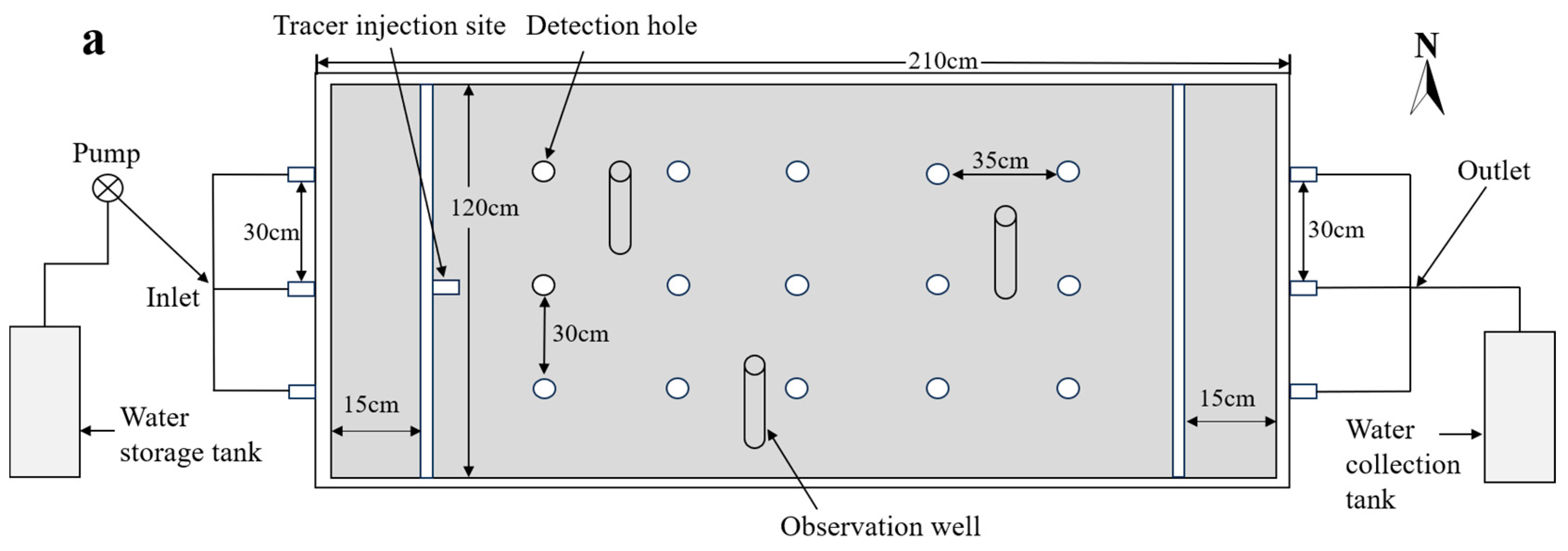
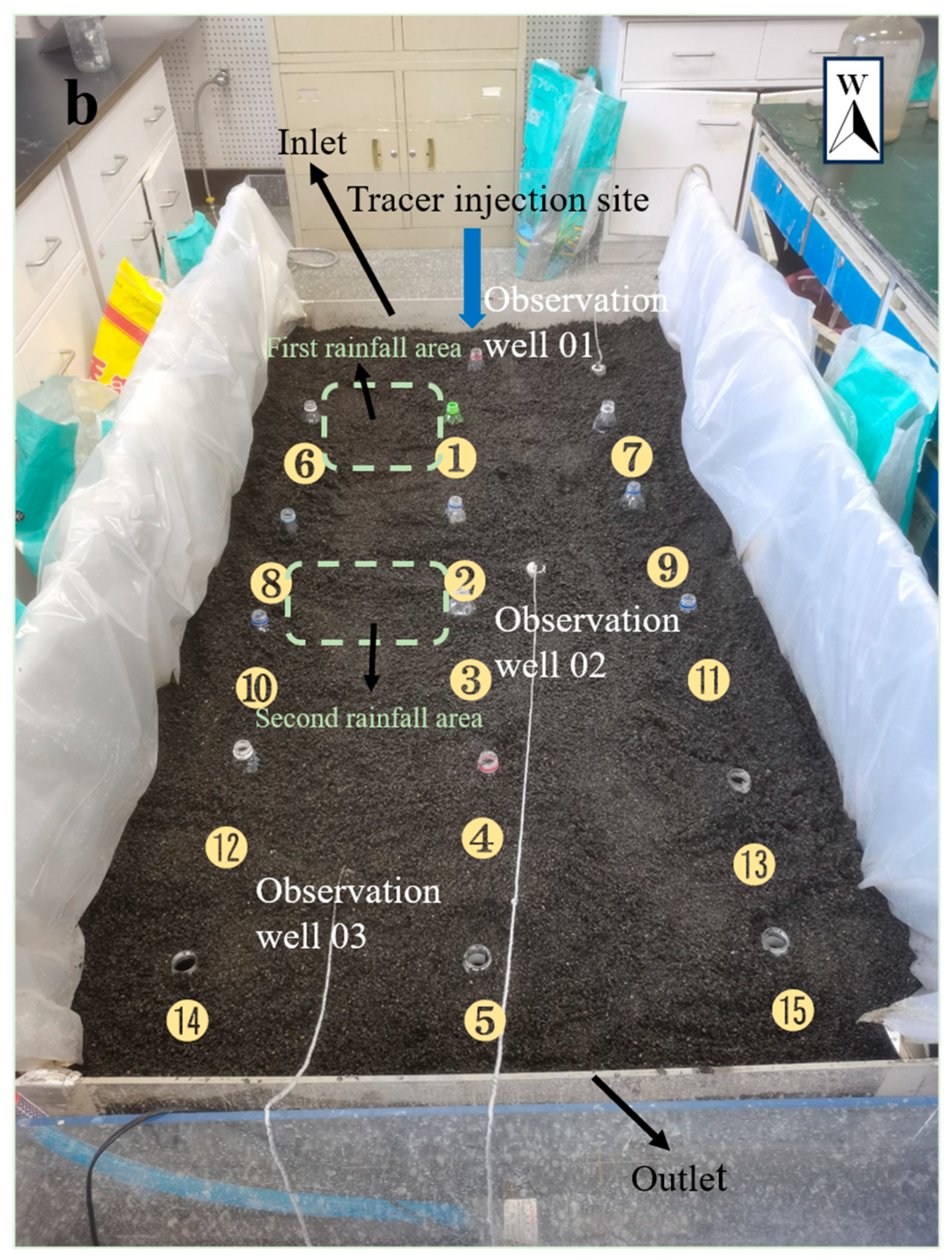
2.2.1. Experimental Materials and Equipment

Fine-to-medium natural quartz was used as the transport medium, with a median particle size of 0.44 mm. NaCl solution (with a concentration of 17 g/L) was prepared as a tracer. The sand was placed in a water tank to be cleaned repeatedly until the water was clear and free of impurities [18]. Then, the sand was put into an oven to air dry at 150 °C three times; after cooling, the preliminary sand sample was obtained. The sample was further passed through a 60-mesh vibrating screen to obtain the medium-to-fine sand (0.1~0.3 mm) with a density of 1.5 g/m3. After that, the sample was flatly placed in the sand box, and the box was shaken; every 3 cm sand was placed to ensure that the sample at the bottom of the box was free of voids. After the sample was paved to 18 cm, water was injected through the inlet till the water level was up to 10 cm.
The test equipment used for this study is shown in Figure 1. The test equipment, which is 2.4 m in length, 1.2 m in height, and 0.6 m in width, was made of 7 mm-thick tempered glass and sealed with Teflon glue and silica gel. An inlet and outlet were installed in front of and behind the test equipment, respectively. Both the inlet and outlet were located about 0.15 m from the front and back ends of the flow cell. A tracer injection port was installed on the inlet side. One side of the flow cell (the inlet side) was raised by 2 cm to achieve a hydraulic gradient of 5‰. The sealed flow cell was then filled with natural quartz to a thickness of 18 cm [19]. Next, the sand-packed flow cell was sprayed with water to remove any impurities introduced during the filling process or present in natural quartz itself. Water was injected into the sand-packed flow cell using a piston pump, with the flow rate set to 2 L/min. Water injection stopped when the water level reached 10 cm to simulate the water table aquifer. On the upper boundary of the medium and in the flow direction, one observation well was set up in the upper, middle, and lower positions, respectively. A HOBO water level logger was placed into each well. It was ensured that the three observation wells were not located along one straight line, but rather at the three vertices of a triangle to determine the water table. Along the upper interface of the medium, 15 tracer concentration detection holes were arranged uniformly. The holes aligned in a straight line with the tracer injection port were primary holes, and those on either side were secondary holes. At a height of 20–30 cm above the medium, a sprinkler head was installed to simulate precipitation. The ambient temperature was controlled at (23 ± 1) °C to ensure that the experiment proceeded smoothly. The key parameters of the flow cell are shown in Table 1. A mild precipitation rate (0.1006 m3/h) and a long-length time step to detect the water level were selected to prevent the formation of groundwater mound.

2.2.2. Experimental Methods

1.
Determination of hydraulic conductivity and porosity
First, the hydraulic conductivity of the medium was determined using a soil column infiltration test device through a constant head hydraulic conductivity test. The inside of the soil column infiltration test device was packed with sand to a height of 18 cm (with a cross-sectional area of 78.5 cm2). The valve was turned on so that the water passed through the sandy medium from top to bottom, and the water was finally discharged from the outlet. After the difference in the hydraulic head Δ h and the seepage quantity Q stabilized, the quantity Q 1 of water flowing through the medium within time Δ t was determined. Then, we estimated the hydraulic conductivity k of the medium to be 12 m/d using Darcy’s law.
Next, the porosity of the sandy medium was measured using the oven drying method. First, the medium sample (1200 g) was placed into an oven and dried continuously at 120 °C for 12 h until the sample was completely dry. The sample was taken out, left to cool, and injected with water until saturation. The volume ratio of water to the medium sample was measured to obtain the medium porosity of 0.4445. The key parameters of the medium are shown in Table 2.
2.
Determination of gradient of water table
Water was injected into the sand layer via the inlet. The outlet was opened when the water level rose steadily to 10 cm above the ground. The inlet flow rate was adjusted so that the water table stabilized at 10 cm above the ground. The test for measuring the gradient of the water table without precipitation lasted 45 min. During the test, data were acquired by each of the three water level loggers once every 3 min. Water table data at three different positions of the water table aquifer—namely, the upper, middle, and lower regions—were collected simultaneously using the three water level loggers. In this way, we obtained the instantaneous equation for the water table position. The correct instantaneous water table equation could be derived by setting the sampling frequency to once every three min. In addition, we observed the changes in the gradient of the water table in the absence of precipitation.
The test for measuring the gradient of the water table with precipitation lasted for 40 min, with a precipitation intensity of 0.1006 m3h−1. The three water level loggers were configured to collect data once every 20 s. Thus, 363 groups of data were collected during the experimental period. Measures were taken to prevent the outcrop of the aquifer in areas exposed to precipitation, which was important for preventing the formation of surface runoff, thereby ensuring experimental accuracy. First, the sandy medium was sprayed with water to simulate precipitation in the upstream position of the flow cell in the flow direction. Subsequently, the medium was sprayed uniformly with water in the middle position for 15 min. The intensity of the two precipitation episodes remained constant, and the total area affected by precipitation was 0.16 m2. Both precipitation episodes lasted for 15 min. The sampling frequency of the three water level loggers was further increased to obtain more water level data during the precipitation. These data can be used to improve the simulation of the changes in the gradient of the water table with precipitation. Moreover, the water table aquifer had already reached a steady state before the two precipitation episodes. Therefore, the precipitation was sufficient to induce significant changes in the aquifer.
The water table data measured in the three observation wells with and without precipitation were substituted into Equation (1) in Section 2.1 to determine the time-varying gradient of the water table under the two precipitation conditions.
3.
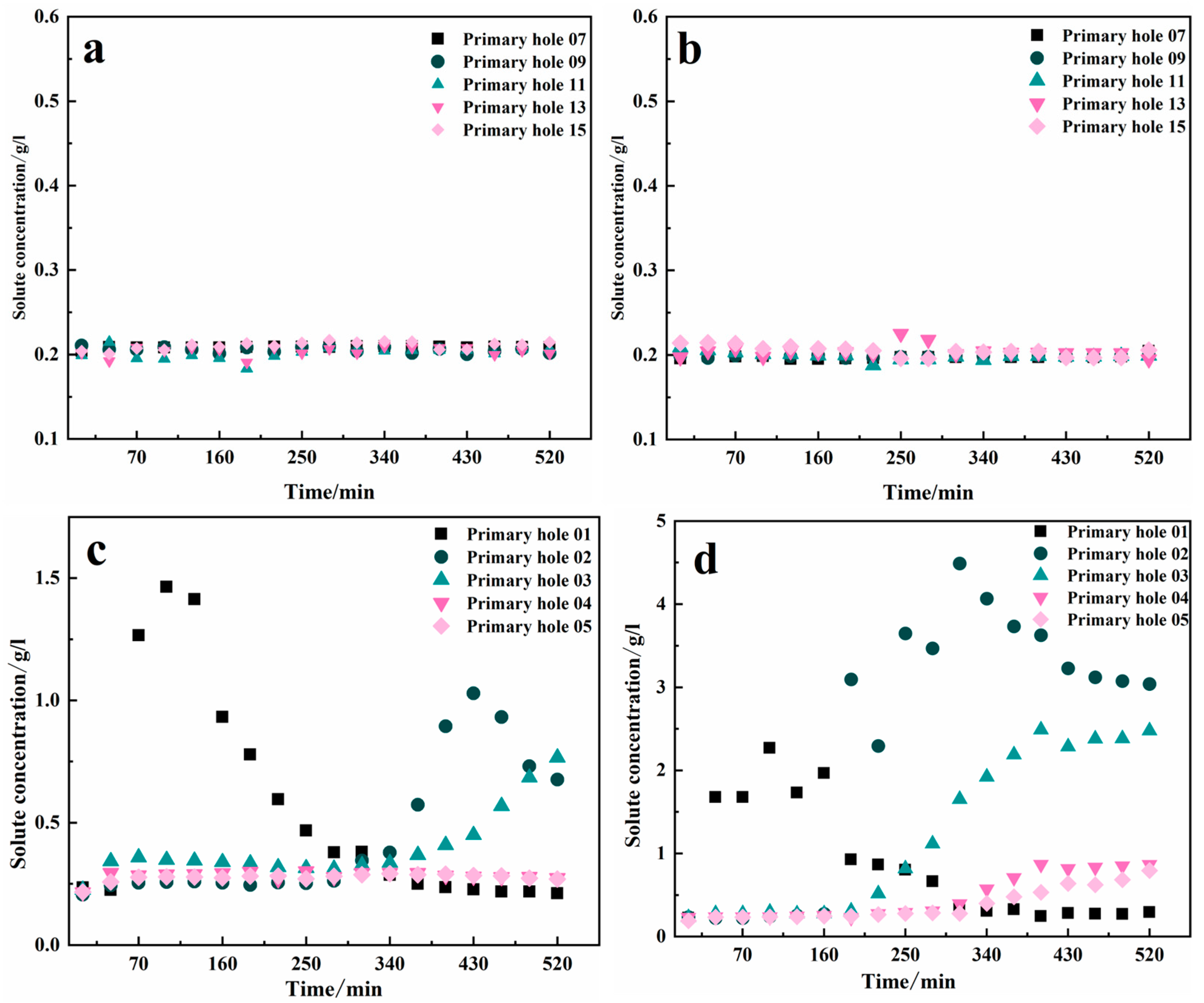
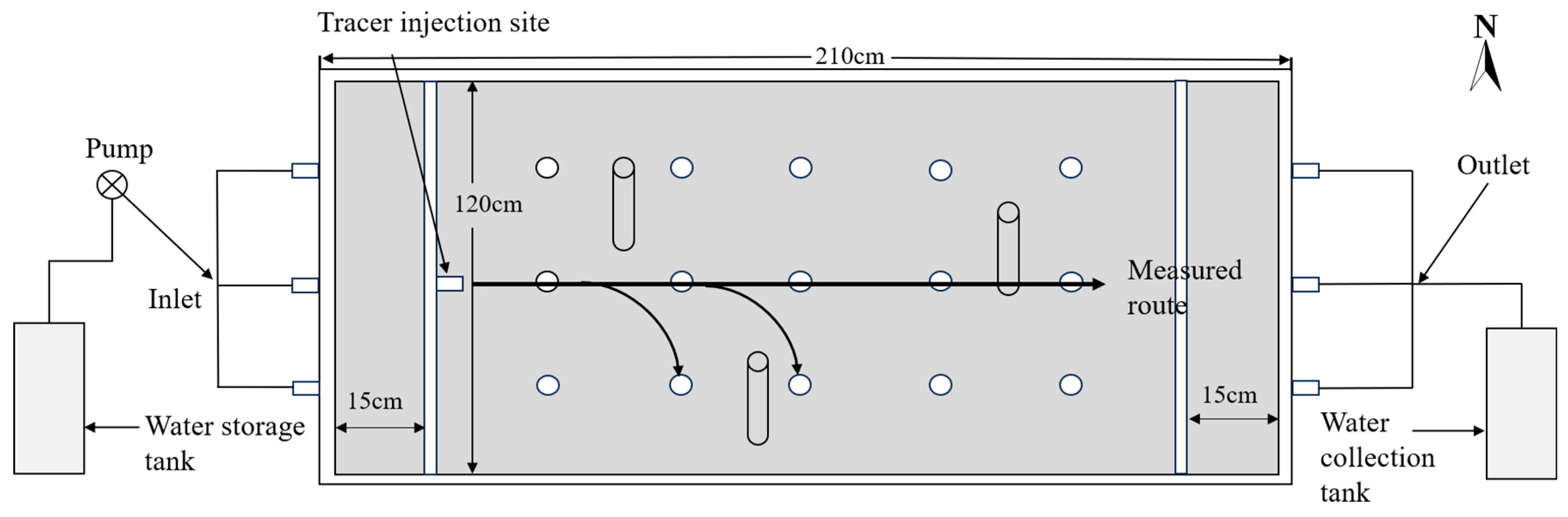
Determination of tracer concentration and route of tracer transport
The test lasted for 12.5 h, and the time interval for data collection by the three water level loggers was consistently 30 min. The blank concentration of water injected into the sandy medium was 0.25 g/L, and the concentration of the injected tracer was 17 g/L. In the first 4.5 h, the tracer concentration was determined once every 30 min, and nine groups of data were collected in total. In the next 8 h, the tracer concentration was determined once every 1 h, and eight groups of data were collected. The water table data and the corresponding tracer concentration data were introduced into the mathematical model in Section 2.1 to obtain the route of the tracer transport at different time steps. See Section 3.3.
The duration (12.5 h) and precipitation intensity (0.22 m3/h) were the same for the tracer transport experiment with and without precipitation. Water table data were collected using the three water level loggers at a time interval of 1 min. The first precipitation episode began when the experiment had proceeded for 130 min. This episode lasted for 15 min and stopped when the experiment had continued for 145 min. The water table began to recover, and the water table data were collected continuously despite the discontinuation of precipitation. The second episode lasting for 15 min began when the experiment had continued for 155 min. The two episodes were spaced 10 min apart.

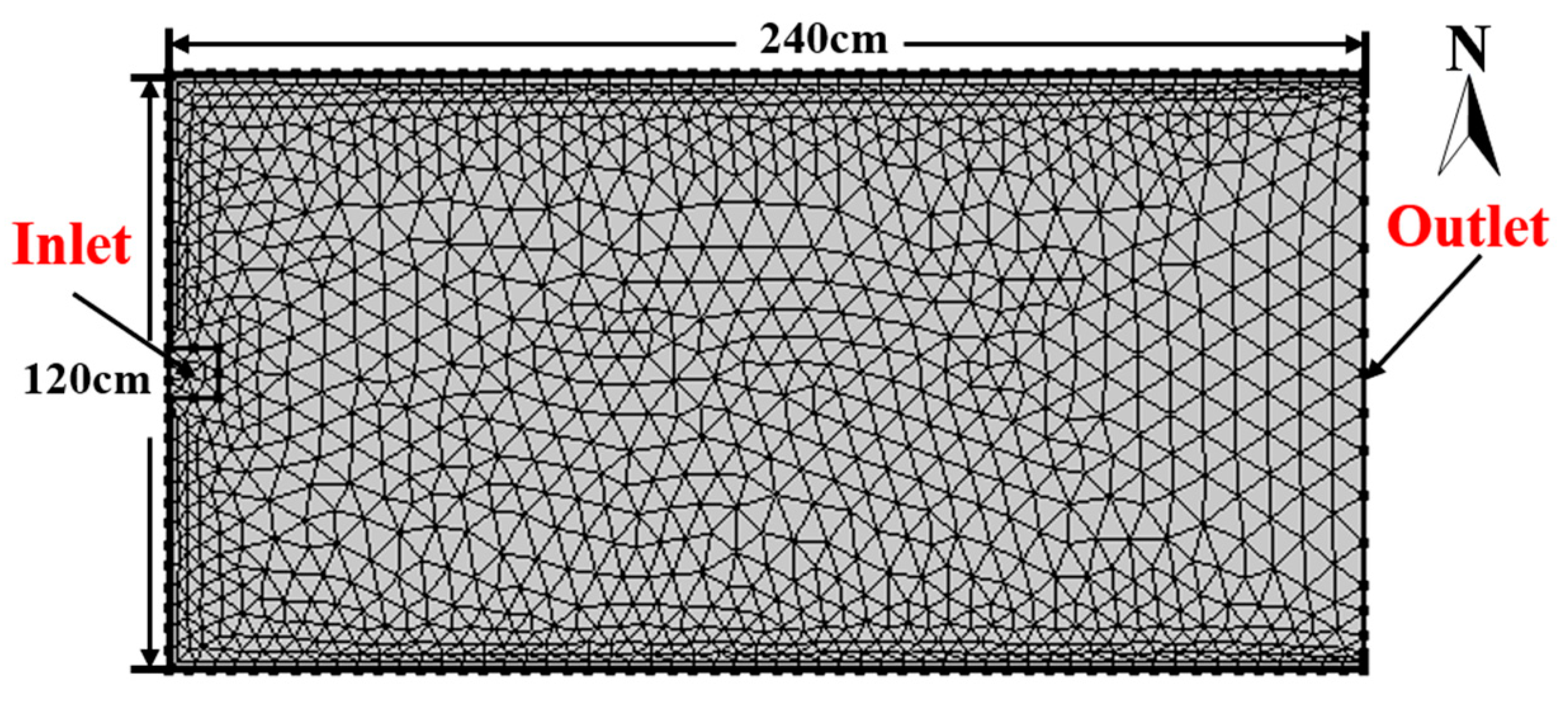
2.3. Numerical Model

To test the reliability of the analytical model, COMSOL Multiphysics 6.0 was employed to simulate the route of the tracer transport with and without the influence of precipitation. The elements and grid set up in the model are presented in Table 3 and Figure 2. The dimension of the model, which was 120 cm × 240 cm, was determined using the same method as the physical model. The laminar module and fluid flow tracking module were applied to simulate particle tracking with and without the influence of precipitation, respectively. Without the influence of precipitation, the velocity field was used to control the variation in velocity. Based on the hydrogeology data from the physical model, the velocity field can be obtained. Then, the route of the particle transport can be simulated given the length of the time step. For the condition with the influence of precipitation, the time-varying gradient of the water table from the physical model needs to be imported into the numerical model to solve the route of the particle transport. The transient solver was applied to acquire the distribution of particles with different velocities. The stability calculation method and mesh refinement processing were employed to guarantee the accuracy of the modeling results. The tolerance was set as 0.01.
The laminar flow module in COMSOL was employed to simulate groundwater flow. The velocities with and without precipitation were entered into the module to simulate groundwater flow. The velocity was calculated based on Darcy’s law. Because coefficients A and B in Equation (1) represent the gradient along the x - and y -directions, respectively, the velocities along the x - and y -directions can be calculated once A and B are obtained. The velocities were then entered into the module to track the particles, and the results were compared with those from the analytical model.

3. Results

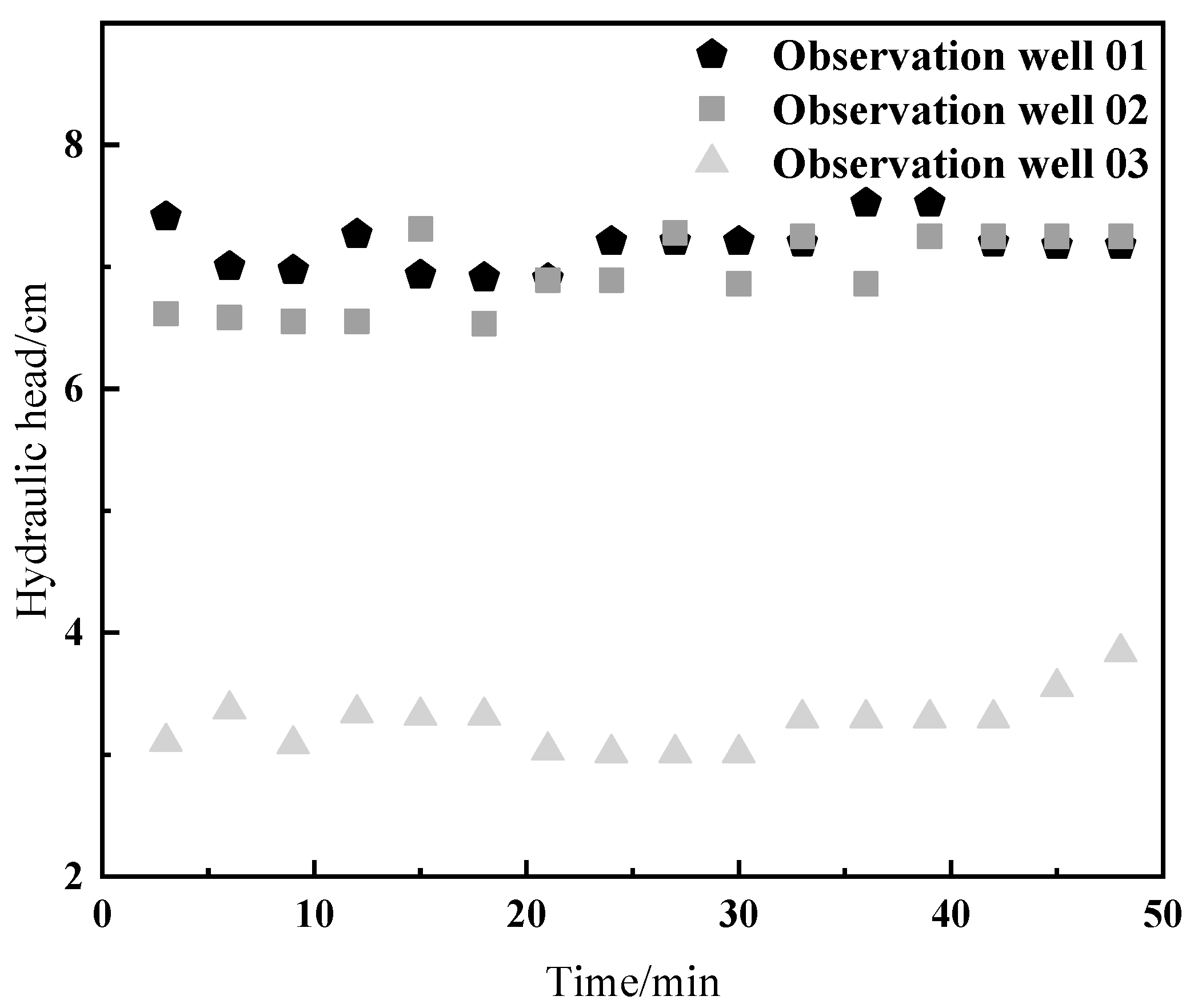
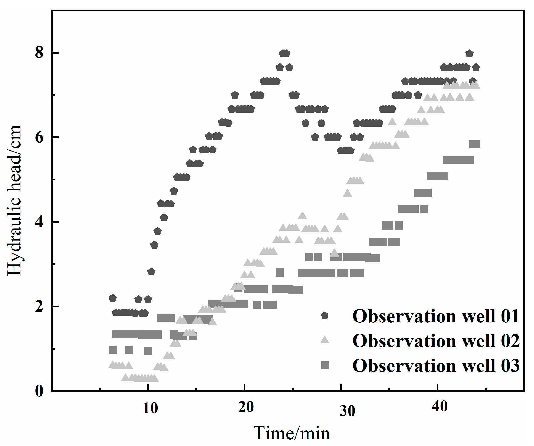
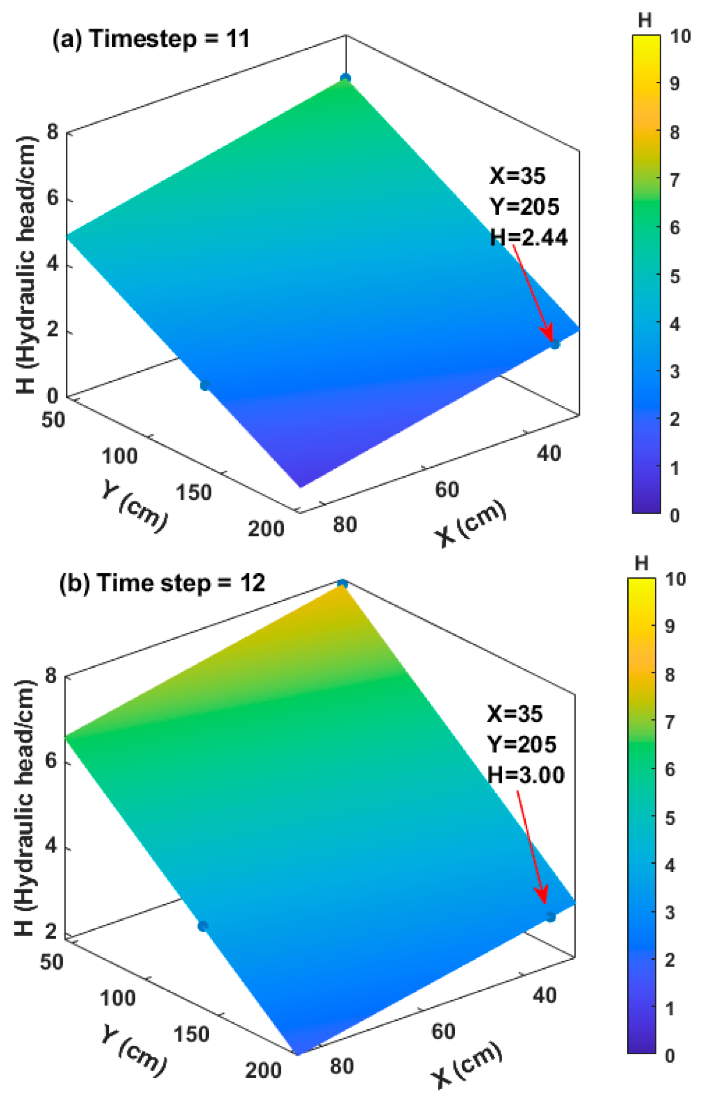
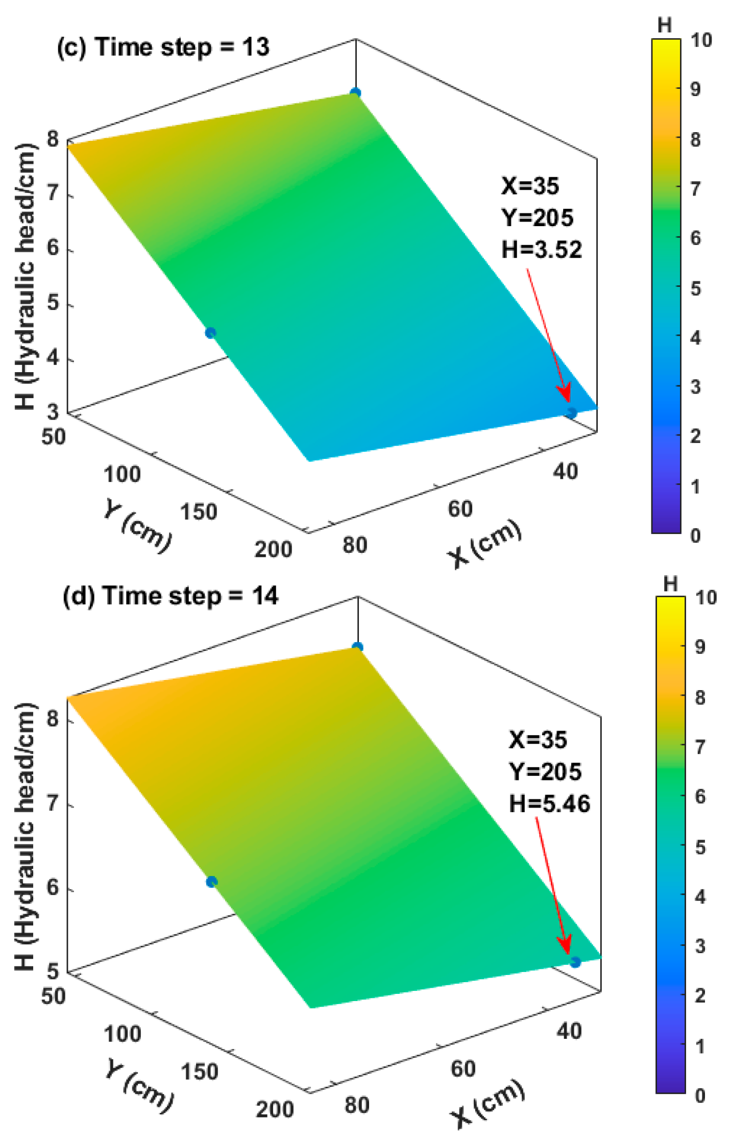
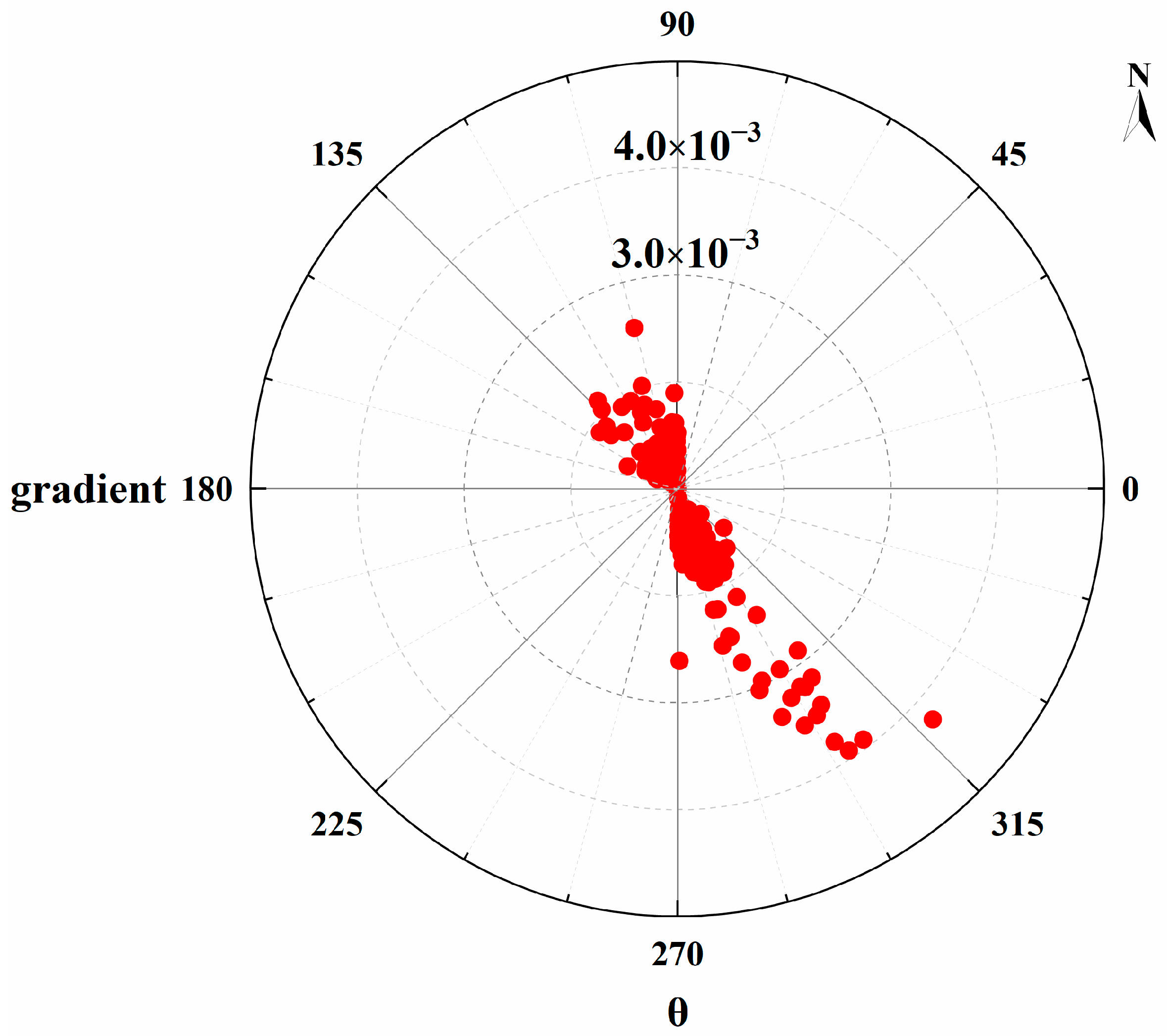
3.1. Changes in the Gradient of Water Table in the Absence of Precipitation

The water table data in the three observation wells in the absence of precipitation are shown in Figure 3. The water table data measured by the three water level loggers fluctuated within narrow margins. Specifically, each group of measurements fluctuated by less than 1 cm.
Figure 4 shows the results obtained from the mathematical model in Section 2.2 at four consecutive time steps. If the same water level data were selected, e.g., (30, 195), the biggest range of variation in the water level is only 0.38 cm, which is quite slight. Hence, these results also demonstrated a slight variation in the gradient of the water table over time without precipitation.

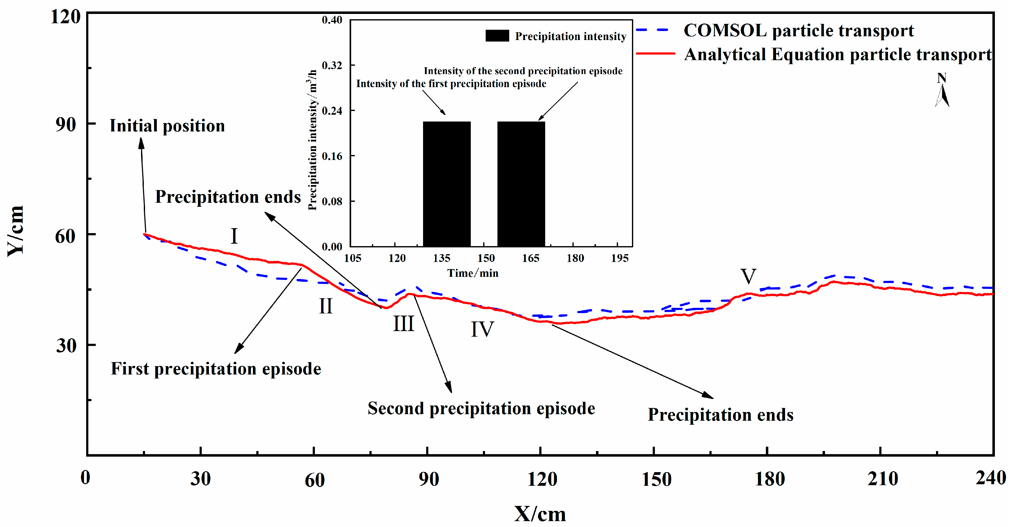
3.2. Changes in the Gradient of Water Table with Precipitation

The water table data in the three observation wells with precipitation are shown in Figure 5. The water table data measured in the three observation wells varied dramatically. The water table in observation well 01 varied within the range of 939 cm to 945 cm. The water table in observation well 02 varied within the range of 938.5 cm to 943 cm. The water table in observation well 03 varied within the range of 937.5 cm to 945 cm. The water table data rose more quickly in observation wells 01 and 02, which lay closer to the areas exposed to precipitation. By contrast, observation well 03 was further away from the areas exposed to precipitation, and the water table rose slowly.
Figure 6 shows the changes in the gradient of the water table at four consecutive time steps with precipitation. In this case, for the first time step, if the water level data at the same point as that of Figure 3 were selected, the water level was lifted from 6.65 cm to 7.66 cm. For the second time step, the water level was lowered due to the impact of precipitation. This was similar to the water level in the subsequent time steps. The gradient of the water table changed more significantly in the presence of precipitation, which indicated the importance of precipitation in changing the gradient of the water table.

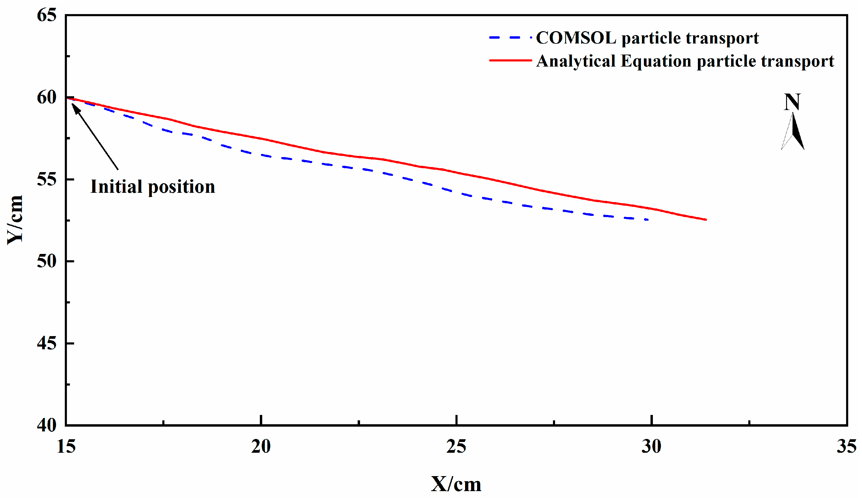
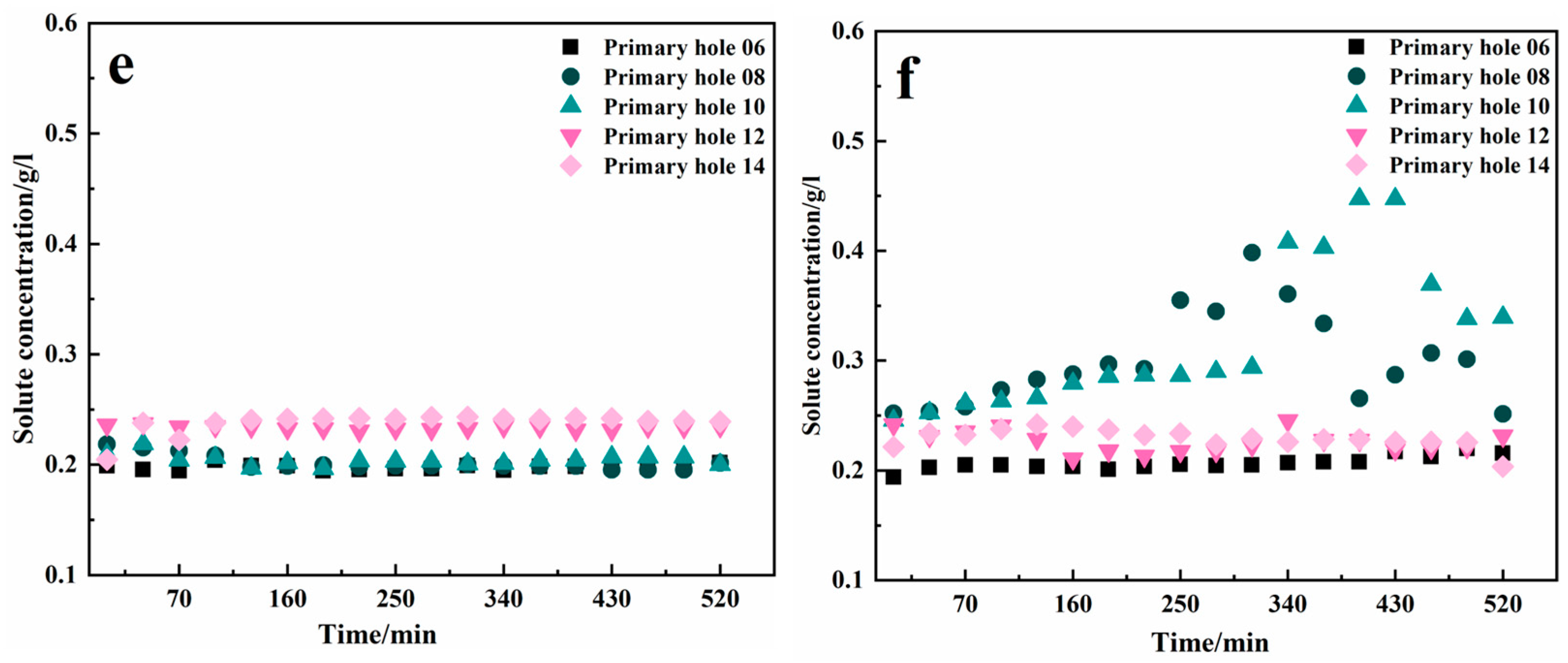
3.3. Simulation of Tracer Transport Routes

During the same period, changes in the gradient of the water table and the route of the tracer transport are shown in Figure 7 and Figure 8, respectively. Figure 7 shows the magnitude of the hydraulic gradient in each direction from the experiment over the study period. The center of the circle represents the starting point of the groundwater or a fluid particle. The red points in the figure indicate the directions and magnitudes of the hydraulic gradients for the groundwater or fluid particles flow from the starting point. In Figure 7, the direction of the gradient mainly ranges from northeast to southwest. Without precipitation, the gradient of the water table changed slightly over time. Gradients with a higher magnitude are mainly distributed along the northwest–southeast 330–345 ° . As the tracer transport is mainly driven by the gradient, the tracer was primarily transported in the flow direction along the sandy trough (Figure 7, northwest–southeast 330–345 ° ). The slight variation of water table had almost no impact on the path of tracer transport. The tracer changed its route slightly along the route.
The simulation results for the route of the tracer transport through a numerical model is shown in Figure 8. There are 4% and 0.2% deviations between the two models for the x -direction and y -direction, respectively. The transportation routes predicted by the two models are similar—which both present the northwest–northeast direction—indicating that the prediction from the analytical model is reliable.
The changes in the gradient of the water table with precipitation are shown in Figure 9. In Figure 9, although the directions of the hydraulic gradient are diversified in other directions with different magnitudes, the higher magnitudes are mainly distributed along the northeast to southwest direction. It is suggested that the gradients of the water table are influenced by the limited number of precipitation events. The route of the tracer transport within the same period is shown in Figure 10. While the tracer was transported in the flow direction along the sandy trough, the route deviated toward the northwest–southwest direction by 0.4 m. It can be found from Figure 9 and Figure 10 that the route of the tracer transport was consistent with the direction in which the gradient of the water table changed. At the initial stage of particle transport (stage Ⅰ, 0 min to 130 min), the route barely changed as the gradient of the water table changed very slightly. At this stage, the route of the particle transport was mainly controlled by the flow direction along the sandy trough. The first precipitation episode occurred at stage Ⅱ (130 min to 145 min) and changed the gradient of the water table. As a result, the route of the tracer transport deviated compared with the situation at stage I. After the precipitation stopped (10 min), the route of the tracer transport changed considerably at stage III (in the northeast–southeast direction). Subsequently, the second precipitation episode began (155 min), which exerted further impact on the gradient of the water table. The route of the tracer transport was also altered (northwest–southeast 285–300 ° ). The second episode ended 15 min later, and stage Ⅴ began, with a mild change in the water table. Moreover, the route of the tracer transport was no longer deviated as before (northwest–southeast 330–345 ° ).
The results from the numerical model are shown in Figure 10. For the first precipitation period, the direction of the routes of the particle transport from the two models are both along the northwest–southeast direction. The distances that the particle moved along the x -axis and y -axis for the analytical and numerical models are 11.44 cm, 22 cm and 10 cm, 29 cm, respectively. The discrepancies are 0.0005% and 17% at the x -axis and y -axis between the two models. For the second precipitation period, the route of the particle transport obtained from the two models are similar. The deviations between the two models are small: there are 0.001% and 0.003% discrepancies for the distances the particle moved along the x - and y -axis, respectively. Even though small discrepancies existed between the two models, the routes of the particle transport from the two models are almost the same, indicating that even under the precipitation conditions, the analytical model employed in this study could be reliable and this analytical model could be used to predict solute transport under changes in the gradient of the water table.
Figure 11 shows the variation of the tracer concentration over time. For the condition without the influence of precipitation, dramatic changes in the tracer concentration mainly occurred in holes 1 and 2. At the beginning of the injection, a high concentration was detected in hole 1 and the concentrations in the other four holes (2–4) remained low (Figure 11b). Then, the concentration in hole 1 gradually decreased as the tracer mainly moved to the next holes along the longitudinal direction. Correspondingly, the concentrations in holes 2 and 3 gradually increased. Lower concentrations were measured in holes 4 and 5 due to the dispersion, but these concentrations were still higher than the paralleled holes, 12–15. The tracer concentrations in holes 6, 7, 8, 9, 10, 11, 12, 13, 14, and 15 remained at low values and stable (Figure 11a,e). The results indicate that without the influence of precipitation, the tracer mainly moved along the longitudinal direction, which is driven by topography.
For the condition with the influence of precipitation, along the longitudinal direction, the changes in the concentration in holes 1 and 3 showed similar trends compared with those from the condition without the influence of precipitation (Figure 11d). The concentration in hole 2 varied significantly during the experiment due to the changes in the gradient of the water table (Figure 6). Also, as holes 2–4 are located in the central part of the aquifer, the changes in the gradient of the water table had a greater impact on these three holes. Compared with the results in the absence of precipitation, the concentrations in holes 3 and 4 were both gradually increased due to the influence of the time-varying gradient of the water table. A low concentration was detected in hole 5, which suggests that the higher amount of tracer may not move there.
Variations in the concentration were also detected in holes 6–10 (Figure 11f). More significant changes in the concentration close to the end of the experiment in these three holes show that the tracer moved to the southeast direction after initially moving along the longitudinal direction. The lower concentrations detected in holes 7–15 indicate that the tracer may not move in the northern part of the aquifer (Figure 11b). In general, the route of the tracer changed with the time-varying gradient of the water table under the influence of precipitation. The route was consistent with the results from the model. For the condition without the influence of precipitation, the route is mainly along the longitudinal direction. The water level data obtained from the lab experiment were imported into the analytical model. Compared with the results from the lab experiment, the route from the model deviated a little to the southeast direction (Figure 8). To predict the route of the particle transport, the hydrogeological condition of the sandy aquifer in the physical experiment was assumed as homogeneous and isotropic. However, in the lab experiment, the homogeneity of the aquifer cannot by formed. Therefore, the heterogeneity of the aquifer could influence the route of particle transport. This is the reason why there is a deviation between the model and lab experiment.
Based on the results from the lab experiment and the model, the two scientific questions proposed in the introduction section have been answered: precipitation could have an impact on the gradient of the water table, and the route of solute transport could be influenced by this changing gradient of the water table.

4. Discussion

The impact of fluctuations in the water table on solute transport has been investigated by researchers. As mentioned above, Attie et al. [13] and Boumaiza et al. [14] used modeling to analyze instantaneous changes in the NAPL thickness in water wells caused by water table fluctuations. Guo et al. [9] found that water table fluctuations shortened or elongated the transport route of the dissolved phase in the NAPL. In addition, Pan et al. [16] used a numerical multiphase flow model for a vadose zone to show that changes in the moisture content due to water table fluctuations had direct controlling effects on the transport law and distribution characteristics of the NAPL. These studies indicate that water table fluctuations could have an impact on solute transport. A fluctuation in the water table refers to changes in the water table in the vertical direction. Under this condition, either the gradient of the water table would change slightly or no variations would occur in the gradient of the water table. Assuming that particles are placed on the water table or the saturated zone, the flow path of the particles could not change due to the constant gradient of the water table. However, whether changes in the gradient of the water table within a specific region has an impact on the solute transport process in groundwater still needs to be explored. Gao [20] reported that hydrological process, e.g., changes in the river stage in an adjacent river, could change the gradient of the water table throughout the years. He developed an analytical model and used water level data collected in a petroleum fuel terminal in Kansas City, Missouri, to simulate particle tracking near the Missouri River with variable river stages. He showed that during the period experiencing high and low stages, the flow path of particles would have obvious changes and the particle would not move in the original direction. Also, particles would move along the original direction when the high and low stages do not occur. Hence, he suggested that the variations in the stage in an adjacent river could change the gradient of the water table in the aquifer.
In this study, we aimed to investigate whether other hydrological processes, e.g., precipitation, could have an impact on the gradient of the water table and solute transport. The advection process is the focus of this study. The dispersion and diffusion processes could be analyzed in future research. It is believed that fluctuations in the water table slightly occurred during the experiment, while the flow path of the tracer did not change without the influence of precipitation. On the other hand, changes in the gradient of the water table occurred once the precipitation began or ended, and the tracer did not move in its original direction during these periods. As the number of precipitation events were limited in the experiment, the main moving direction of the tracer was northwest–southeast. Hence, in addition to the water table fluctuations reported in the previous research mentioned above, this study further analyzed whether the hydrological process could impact the regional gradient of the water table. For this study, at the beginning and end of the precipitation events, the moving directions of the tracer changed from its original one. But between the two ends and after the ending of precipitation, the tracer moved along the original direction. Therefore, the results further indicate that under a precipitation event, the gradient of the water table might not be influenced by the whole precipitation process, while the beginning and end of the precipitation event could have an impact on the gradient of water table and, correspondingly, the solute transport. The results further explore the mechanisms of solute transport under precipitation events.
Although the general moving direction of the tracer could be obtained from the lab experiment (Figure 12), the detailed route is still not clear based on the current detection resolution, which is also the limitation of this study. High resolution detection devices will be set in the experiment to be able to measure the concentrations throughout the aquifer in future research.
Numerical models have been widely employed to track the movement of fluid particles, depending on spatial and temporal discretization; however, they may not be able to capture dynamic aspects of groundwater flow for complex water surfaces with dynamic water levels. Specifically, for complicated boundary conditions, numerical models are the first choice to resolve particle tracking, even though they only contribute proximate answers; however, compared to numerical models, particularly for some simple boundary conditions, temporal and spatial discretization in numerical simulations may be insufficient for accurately tracking particles. Analytical methods are useful techniques that can be applied to many ground water flow problems. The analytical model employed in this study is a novel and precise method for tracking particles using continuous water level data, which can be obtained from a field site or a lab experiment, providing an efficient tool for predicting the movement of subsurface contaminants by tracking particles.

5. Conclusions

In this study, we employed an analytical solute transport model under a time-changing gradient of the water table, which was then verified through experiments. The modeling results were compared with those from a numerical model to analyze the modeling reliability. On this basis, we investigated the mechanism by which the time-varying gradient of the water table influenced the solute transport process. The results showed that:
(1)
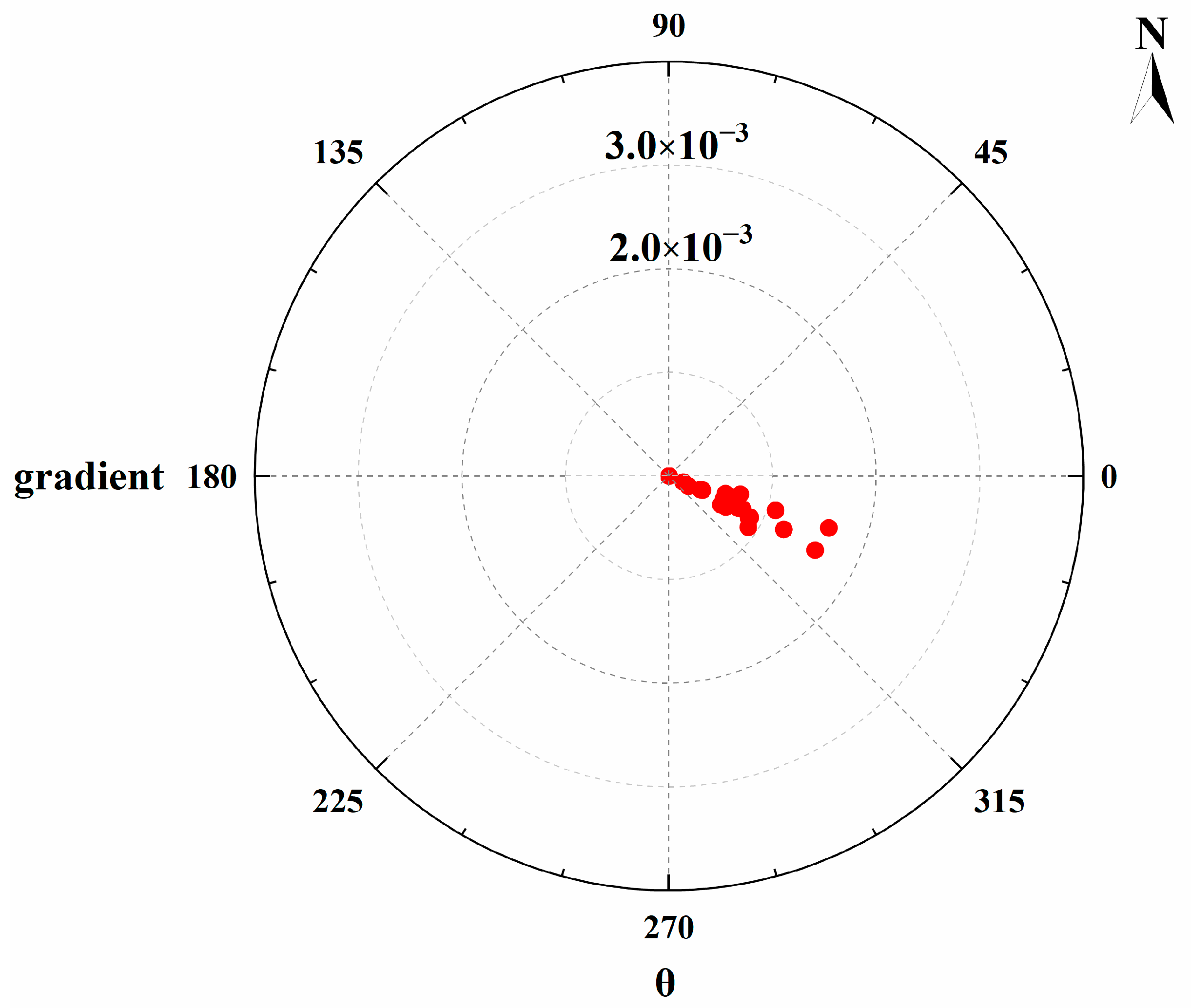
Precipitation did have an impact on the gradient of the water table within a specific region. The gradient of the water table barely changed over time without precipitation.
(2)
The changing gradient of the water table had a large bearing on the route of the tracer transport. The tracer was mainly transported along the flow direction along the sandy trough. The stable water table hardly had any impact on the route of the tracer transport. As the gradient of the water table changed dramatically with the influence of precipitation, the route of the tracer changed correspondingly.
(3)
For future experiments, by shortening the time interval for collecting data to determine the changes in the gradient of the water table using water level loggers, the accuracy of the model in simulating the route of solute transport in an aquifer could be improved.
In this study, the main objective was to highlight the impact of precipitation on the gradient of the water table and to analyze how solute transport in an aquifer could be influenced by this changing gradient of the water table. Hence, some hypotheses have been made—e.g., the aquifer is homogeneous and isotropic—to calculate the route of particle transport to highlight the influence of precipitation on the gradient of the water table. Therefore, although the numerical model was also used to test the reliability of the analytical method, there were still limitations. The hypothesis presented in this study is an ideal condition, which has little reference to real conditions. Further, the physical experiment was conducted in the lab. The results also have discrepancies with those obtained from the fieldwork. For this model to better reflect real conditions, practical, in-situ testing, such as a pumping test, needs to be conducted in order to acquire real hydraulic conductivity values and other hydrogeological data in future research. Also, adsorption, chemical reactions, and retardation factors, as well as in-situ data, need be put into this analytical model for the predictions to be more applicable to the real conditions. We did not pay attention to the hydrogeology conditions in this study. However, precipitation can occur anywhere, so the gradient of the water table can be impacted by precipitation universally. Researchers and engineers could apply this analytical model by importing local hydrogeological data obtained from pumping tests or other in-situ data to predict solute transport much more precisely.

Author Contributions

Conceptualization, Y.G. and L.D.; methodology, Y.G. and L.D.; software, Y.G. and X.Z.; validation, L.D.; formal analysis, L.D. and X.Z.; investigation, Y.G. and L.D.; resources, Y.G.; data curation, L.D., J.S., Z.Z., Z.L., P.G. and X.Z.; writing—original draft preparation, L.D. and X.Z.; writing—review and editing, Y.G., L.D. and X.Z.; visualization, X.Z.; supervision, Y.G.; project administration, Y.G.; funding acquisition, Y.G. All authors have read and agreed to the published version of the manuscript.

Funding

This research was funded by the National Undergraduate Training Program for Innovation and Entrepreneurship, grant number 202210755008 and the Natural Science Foundation of Xinjiang Uygur Autonomous Region, grant number 2022D01C40.

Data Availability Statement

The general data are included in the article. Additional data are available on request.

Acknowledgments

We acknowledge the National Undergraduate Training Program for Innovation and Entrepreneurship and the Natural Science Foundation of Xinjiang Uygur Autonomous Region for funding this project.

Conflicts of Interest

The authors declare no conflict of interest.

References

  1. Wang, Z. An analysis of China’s main pathways of and preventive measures for groundwater pollution in China. Technol. Econ. Guide 2016, 23, 1–2. [Google Scholar]
  2. Tang, W. A study on the application of modified porous ceramics in water treatment. Jingdezhen Ceram. Inst. 2020, 1–3. [Google Scholar]
  3. Chen, Z.; Xie, S.; He, C. Status quo and development tendency of the simulation technology for contaminant transport in the shallow groundwater. J. Univ. South China Sci. Technol. 2005, 19, 6–10. [Google Scholar] [CrossRef]
  4. Xu, W. Influence of groundwater seepage on pollutant transport and a predictive research. Ind. Water Wastewater 2018, 49, 3–6. [Google Scholar] [CrossRef]
  5. Fischer, H.B.; List, E.J.; Koh, R.C.Y.; Imberger, J.; Brooks, N.H. Mixing in Inland and Coastal Waters; Academic Press: San Diego, CA, USA, 1979; pp. 350–361. [Google Scholar] [CrossRef]
  6. Mc Clain, M.E. Biogeochemical hot spots and hot moments at the interface of terrestrial and aquatic ecosystems. Ecosystems 2003, 6, 301–312. [Google Scholar] [CrossRef]
  7. Pollock, D.W. Semianalytical computation of path lines forfinite-difference models. Groundwater 1988, 26, 743–750. [Google Scholar] [CrossRef]
  8. Keefe, S.H.; Barber, L.B.; Runkel, R.L.; Ryan, J.N.; McKnight, D.M.; Wass, R.D. Conservative and reactive solute transport in constructed wetlands. Water Resour. Res. 2004, 40, 40–41. [Google Scholar] [CrossRef]
  9. Harvey, J.W.; Saiers, J.E.; Newlin, J.T. Solute transport and storage mechanisms in wetlands of the Everglades. Water Resour. Res 2005, 41, 41–53. [Google Scholar] [CrossRef]
  10. Islam, M.; Azaiez, J. Miscible thermo-viscous fingering instability in porous media. Transp. Porous Media 2010, 84, 845–861. [Google Scholar] [CrossRef]
  11. Yuan, Q.; Azaiez, J. Inertial effects of miscible viscous fingering in a Hele-Shaw cell. Fluid Dyn. Res. 2015, 47, 47–53. [Google Scholar] [CrossRef]
  12. Boano, F.; Packman, A.I.; Cortis, A.; Revelli, R.; Ridolfi, L. A continuous time random walk approach to the stream transport of solutes. Water Resour. Res. 2007, 43, 43–55. [Google Scholar] [CrossRef]
  13. Attie, O.; Palmier, C.; Schafer, G. On the influence of groundwater table fluctuating on oil thickness in a well related to an LNAPL contaminated aquifer. J. Contam. Hydrol. 2019, 223, 5–8. [Google Scholar] [CrossRef]
  14. Boumaiza, L.; Chesnaux, R.; Walter, J.; Lenhard, R.J.; Hassanizadeh, S.M.; Dokou, Z.; Alazaiza, M.Y.D. Predicting Vertical LNAPL Distribution in the Subsurface under the Fluctuating Water Table Effect. Groundwater 2022, 42, 47–58. [Google Scholar] [CrossRef]
  15. Gupta, P.K.; Gharedaghloo, B.; Lynch, M.; Cheng, J.; Strack, M.; Charles, T.C.; Price, J.S. Dynamics of microbial populations and diversity in NAPL contaminated peat soil under varying water table conditions. Environ. Res. 2020, 191, 110–167. [Google Scholar] [CrossRef]
  16. Pan, M.; Shi, J.; Zuo, R.; Zhao, X.; Jiu, J.; Xue, Z.; Wang, J.; Hu, L. Numerical simulation study of the effect of the vadose zone with lenses on LNAPL migration under the fluctuating water table. Hydrogeol. Eng. Geol. 2022, 49, 154–163. [Google Scholar] [CrossRef]
  17. Gao, Y. Particle Tracking Using Dynamic Water-Level Data. Water 2020, 12, 2063. [Google Scholar] [CrossRef]
  18. Wang, J.; Qi, Y.; Ma, Y. Study on migration of characteristic pollutants in red mud leachate in saturated sand. J. Environ. Eng. Technol. 2022, 12, 1210–1216. [Google Scholar] [CrossRef]
  19. Ma, S.; Wang, K.; Fu, Z. Application of on-site pumping test to determine the permeability coefficient of aquifer in the engineering field. Soil Eng. Found. 2022, 36, 486–490. [Google Scholar]
  20. Gao, Y. Particle Tracking Using Dynamic Water Level Data. Master’s Thesis, Colorado State University, Fort Collins, CO, USA, 2017. [Google Scholar]
Figure 1. (a) Schematic diagram of test equipment; (b) test experiment used in the lab.
Water 15 03187 g001aWater 15 03187 g001b
Figure 2. Grid setup in the numerical model.
Water 15 03187 g002
Figure 3. Water level data in the three observation wells without precipitation.
Water 15 03187 g003
Figure 4. Changes in the gradient of water table at four consecutive time steps without precipitation.
Water 15 03187 g004
Figure 5. Changes in water table data in the three observation wells with precipitation.
Water 15 03187 g005
Figure 6. Changes in the gradient of water table at four consecutive time steps with precipitation.
Water 15 03187 g006aWater 15 03187 g006b
Figure 7. Variation of gradient of water table without precipitation. The red points in the figure indicate the directions and magnitudes of the hydraulic gradients for the groundwater or fluid particles flow from the starting point.
Water 15 03187 g007
Figure 8. Route of tracer transport without precipitation.
Water 15 03187 g008
Figure 9. Variation of the gradient of water table with precipitation.
Water 15 03187 g009
Figure 10. Route of tracer transport with the influence of precipitation.
Water 15 03187 g010
Figure 11. Variation of tracer concentration over time. (a,c,e) Variation of tracer concentration in detection holes over time without the influence of precipitation; (b,d,f) variation of tracer concentration in detection holes over time with the influence of precipitation.
Water 15 03187 g011aWater 15 03187 g011b
Figure 12. Measured direction of tracer transport.
Water 15 03187 g012
Table 1. Key parameters of flow cell.
Q / mL · min 1 A / c m 2 θ w
200072,00039%
Note Q is the flow rate of the pump; A is the cross-sectional area of the lateral face of the flow cell; θ w is the volumetric moisture content.
Table 2. Physical parameters of the medium.
ρ / g · cm 3 K / m · d 1 φ
1.5120.4445
Note: ρ is the bulk density; K is the hydraulic conductivity; φ is porosity.
Table 3. Mesh parameters used in the numerical model.
Vertex Element NumberBoundary Element NumberNumber of ElementMinimum Cell Mass
817124250.1797
Disclaimer/Publisher’s Note: The statements, opinions and data contained in all publications are solely those of the individual author(s) and contributor(s) and not of MDPI and/or the editor(s). MDPI and/or the editor(s) disclaim responsibility for any injury to people or property resulting from any ideas, methods, instructions or products referred to in the content.

