Article

Life History Traits of the Stygophilous Amphipod Synurella ambulans in the Hyporheic Zone of the Lower Reaches of the Upper Sava River (Croatia)

1
Department of Biology, Faculty of Science, University of Zagreb, Horvatovac 102a, 10000 Zagreb, Croatia
2
Graduate School, University of Nova Gorica, Vipavska 13, 5000 Nova Gorica, Slovenia
3
Ruđer Bošković Institute, Bijenička Cesta 54, 10000 Zagreb, Croatia
*
Author to whom correspondence should be addressed.
Water 2023, 15(18), 3188; https://doi.org/10.3390/w15183188
Submission received: 6 August 2023 / Revised: 4 September 2023 / Accepted: 5 September 2023 / Published: 7 September 2023
(This article belongs to the Special Issue Groundwater and Connected Ecosystems)

Abstract

:
Estimating the growth and population dynamics of crustaceans is important for understanding the role of species in ecosystems and for conservation and monitoring purposes. This study investigated temporal and spatial variation in population dynamics (growth rate, instantaneous mortality rates, and longevity) of the stygophilous freshwater amphipod Synurella ambulans (F. Müller, 1846), and influencing environmental factors. Seasonal sampling was conducted from December 2018 to October 2019 at two sampling sites (Jarun and Medsave) along the Sava River in northwestern Croatia. A Bhattacharya cohort analysis was applied to the length-frequency data using the FISAT software package. At least four cohorts were distinguished during the year. The possible influence of environmental factors on growth parameters was investigated using Canonical Correspondence Analysis (CCA), which revealed that the important environmental factors influencing S. ambulans abundance were water temperature and dissolved oxygen concentration. The average total body length (TBL) of females was 4.25 mm, while the TBL of males was 3.34 mm. The asymptotic length (L) and growth coefficient (K) were estimated to be 6.30 mm and 0.92 year−1 for females and 5.40 mm and 0.59 year−1 for males, respectively, at the Jarun site. L and K were estimated to be 7.20 mm and 0.34 year−1, respectively, for females and 4.00 mm and 1.20 year−1, respectively, for males at the Medsave site. Estimated total mortality (Z) for each sex had higher values for males than females at both sampling sites. The lack of ecological knowledge on S. ambulans populations and relationships with invertebrate communities in the hyporheic zone of the large river ecosystems emphasises the importance of a detailed study for protecting this species and its vulnerable ecotonal groundwater-connected environment.

1. Introduction

Amphipods (class: Malacostraca; order: Amphipoda) belong to the most abundant, diverse, and taxonomically challenging crustacean order, including over 10,500 species occurring in various aquatic and even terrestrial ecosystems, but most live in marine environments [1,2,3]. However, amphipods are a significant component of various freshwater ecosystems, playing a crucial ecological role in nutrient cycling, bioindication, ecotoxicity testing, hosting parasites, and supporting numerous ecosystem services [4,5]. Due to their critical functional role as prey for many macroinvertebrates, fish, birds and even mammals, they are essential for transporting energy and nutrients to higher trophic levels [6], highlighting their ecological importance in aquatic food webs and connecting aquatic and terrestrial environments.

1.1. Distribution Patterns and Ecology of Synurella ambulans

Synurella ambulans (F. Müller, 1846) belongs to the family Crangonyctidae, a diverse, almost exclusively freshwater Holarctic family comprising 249 species and ten subspecies inhabiting mainly subterranean and surface biotopes with groundwater connections [3,7,8]. It may represent a species complex [9], based on its morphological variability [10,11,12]. Even though the species belongs to the cold-stenothermal, photonegative and thigmotactic organisms [13], it is a euryoecious amphipod species widely distributed throughout central, eastern and south-eastern Europe that can live in a wide range of surface ecosystems (lakes, springs, rivers, swamps, ponds) and subterranean realms (hyporheic zone (HZ), hypotelminorheic zone, phreatic interstitial zone, and caves), in both lowland and mountainous regions [12,14,15,16,17] up to 1600 m a.s.l. [18,19]. As a highly adapted subterranean water dweller, the species belongs to eustygophilous inhabitants [20], although the eyeless stygobiotic populations were also documented in European countries [8].
S. ambulans has been recorded in Europe in many countries: Albania [15], Austria [21,22], Belarus [23], Belgium [24], Bulgaria [11], Croatia [15,25], Czech Republic [26,27], Estonia [28], Germany [16], Hungary [15,29,30], Italy [31,32], Latvia [33,34], Lithuania [17], Montenegro [15,35], Poland [11,36], Romania [37,38], Russia [18], Serbia [15], Slovakia [26,39], Slovenia [20,40,41], Switzerland [4,42], Turkey [43], and Ukraine [44]. In Croatia, it has been found in the Dinaric karst region (intermittent Krčić spring in central Dalmatia) [45] and in the Pannonian region [25]. In addition, this amphipod inhabits the hypotelminorheic zone with underlying flysch at higher elevations in Croatia (Medvednica Mountain, 927 m a.s.l.) [19]. Synurella ambulans rarely inhabits deep lakes, but it was found in the karstic oligotrophic lake Vrana on the island of Cres at depths of 50 to 70 m [46]. It has also been recorded in the HZ of the Sava River in eastern Slovenia [40]. Recently published data confirm that S. ambulans is a suitable bioindicator of chronic metal contamination in the HZ of the Sava River, as it accumulates metals from the interstitial water from the HZ [47]. As a small burrower-like inhabitant of deeper sediment, the species is often overlooked during classical macrozoobenthos field surveys [48], and therefore directed and targeted research is crucial for understanding the ecology and life history traits of this species.

1.2. Amphipod Life History Strategy in the Subterranean Environment

The life history traits of subterranean species have been poorly studied due to many obstacles and challenges to accessing their habitats, difficulties in animal collecting, unsuccessful breeding in laboratory conditions, and the rarity of most subterranean species [49,50,51]. There are only a few articles addressing some aspects of the life history traits of S. ambulans [7,11,12], their mouthparts morphology [52], distribution patterns, e.g., [9,17,24,43], and taxonomy [12]. Despite their importance in hyporheic communities [40], there are still significant gaps in our knowledge of groundwater-connected crustaceans’ biology and life history strategies. Moreover, in the Slovenian and Croatian parts of the Dinaric karst, stygobiotic populations (races) of S. ambulans were recorded in assemblages with stygobiotic Niphargus spp. and the cave salamander Proteus anguinus [20,53]. Therefore, detailed data on the biological characteristics of the species are crucial to understanding its position in the functional structure of the groundwater-connected ecosystems (GWCE).
Knowledge of the population structure and dynamics of crustaceans is fundamental to understanding population ecology, the ecological stability of a species, and the protection of aquatic ecosystems [54]. In addition, the effects on growth and reproduction in amphipods can be measured as one of the endpoints in assessing the effects of contaminants [55]. Life history traits such as the number, age and size at maturity, growth pattern, longevity, timing of reproduction, size and sex ratio of offspring, and fecundity of species have been shown to be related and interconnected to many factors and subjects, from habitat geography and behavioural ecology to natural selection [51,56,57,58]. For example, species from cold climates have greater longevity and greater body size, while species from warm climates have shorter longevity and smaller body size [56]. Life histories are also related to lifestyle and adaptive abilities of crustaceans to specific environmental realms [50,51,56,58].

1.3. Methodology for Life History Analyses

Crustaceans lack typical age determination structures such as scales, otoliths, spines, or shells due to the complex process of ecdysis and restricted growth associated with moulting [59,60]. Because their hard exoskeleton does not grow, an estimation of growth and age structure is severely limited. Therefore, indirect approaches have been developed to calculate the age of crustaceans. In recent decades, several new methods have been used to analyse ageing in crustaceans, such as the widely used content of the brain pigment lipofuscin as an accurate indicator of age [61,62], the counting of endocuticle growth bands in gastric mills and eyestalks [63], and the reflex action mortality predictor (RAMP) method used to predict mortality [64]. The amount of lipofuscin pigment is related to physiological age rather than chronological age [65]. However, analysis of this fluorescent age pigment in amphipods (in slow-growing amphipods) has been shown to be a more accurate method for chronological age determination than body size analysis [62]. In some decapods and slow-growing amphipods, lipofuscin has been shown to be a more adequate age predictor than size [66,67,68,69].
One of the most commonly used tools for assessing population parameters of shrimps is FISAT (FAO-ICLARM Stock Assessment Tools) [70,71,72]. FISAT software (version 1.2.2, FAO, Rome, Italy) was initially developed for fish and is still widely used to assess fish stock exploitation, e.g., [73,74,75], or to study changes in the growth rate of fish [76]. The Von Bertalanffy growth function (VBGF) [77] is an appropriate mathematical model used to describe the growth patterns of crustaceans during their life span. Several studies have used this model to measure the growth of crustaceans, such as economically important shrimp [78,79], amphipods [80,81,82,83], mysids [84], isopods [85,86], and decapods [87,88,89,90,91].
Knowledge of the life history of European gammarids in freshwater environments is sparse and fragmentary, with only a few studies in recent years [92]. Nowadays, analyses of population dynamics in crustaceans include not only life history traits (e.g., body size, population density, breeding period, and sex ratio), but a much broader dataset that includes analyses of longevity, mortality, growth rate, age information, and number of generations (cohorts).
The temporal and spatial changes in environmental factors such as temperature and salinity can strongly influence crustaceans’ growth rates and ageing analysis, as specimens of the same age may belong to different length classes [62,93]. Unfortunately, age analysis based on size-frequency histograms in crustaceans can be a density-dependent method in addition to age [94]. Nevertheless, length-frequency analysis is fast, inexpensive, and efficient, especially for small, non-commercial crustaceans. Moreover, neurolipofuscin as an age marker, mostly used in commercial decapods or larger amphipods, requires the dissection of the brain [66,94], which is very difficult to perform in small species such as S. ambulans (adults 3–6 mm, according to Sidorov and Palatov [12]).

1.4. The Aims of the Research

The general aim of the present research was to assess the relationship between the life history traits of the analysed species S. ambulans and their hyporheic habitat requirements. The specific aims of the study were to (i) estimate key population parameters of S. ambulans, including growth and mortality rates, using length-frequency distribution data; (ii) determine temporal and spatial differences in population dynamics and reproductive strategies (sex ratio and the number of cohorts) at two sampling sites in the HZ of the Sava River, Croatia; and (iii) analyse the possible influence of environmental variables on the measured population parameters. Two sampling sites close to each other with different environmental parameters in the HZ of the Sava River were selected to analyse the differences in life history traits and population dynamics according to previously published data on the metal bioaccumulation and energy status of S. ambulans [47,95]. This study provides a first insight into the population dynamics of S. ambulans inhabiting the HZ of the Sava River and a detailed complex overview of their life history traits in general.

2. Materials and Methods
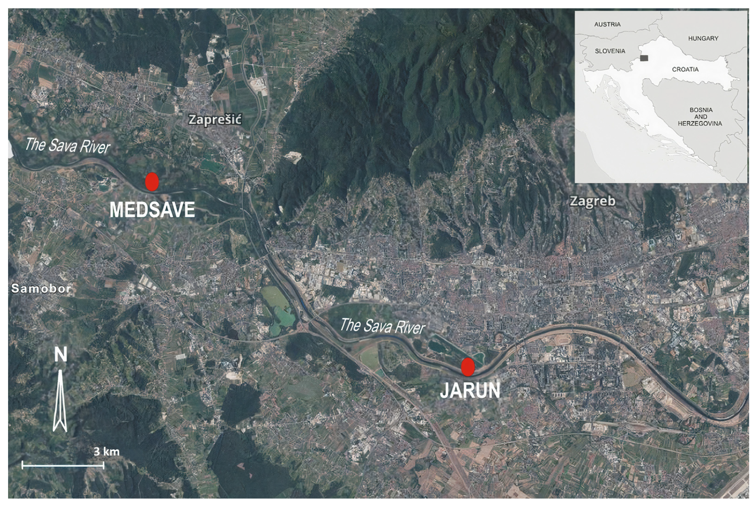
2.1. Study Area

With a total length of 945 km, the Sava is the longest river in the Balkans and one of the most ecologically valuable rivers [96]. Due to the high biodiversity in the wetlands, six sites in the Sava River Basin have been declared Ramsar sites [97]. The Sava River Basin covers a total area of 97,713 km2 [96], spanning the territories of six countries—Slovenia, Croatia, Bosnia and Herzegovina, Serbia, Montenegro, and Albania. It represents one of the most significant sub-basins of the Danube River [97]. Within the Sava River Basin, there are four ecoregions: Alps (ER 4), Dinaric Western Balkan (ER 5), Hungarian Lowlands (ER 11), and Hellenic Western Balkan (ER 6) [98]. High-quality groundwater is the primary drinking water supply in the Sava River basin, which includes two main units: the Pannonian Basin, with intergranular aquifers and the Dinarides, with predominantly limestone aquifers [97]. The Zagreb aquifer system is the only source of drinking water in the city of Zagreb. However, it is threatened by declining groundwater levels and increasing groundwater pollution [99]. In addition, the integrity of the upper and middle sections of the Sava River Basin is threatened by proposed new hydroelectric power plant projects [100,101]. Two study sites in northwestern Croatia, the Medsave and Jarun gravel bars, were selected to determine the biology and habitat ecology of S. ambulans in the HZ of the Sava River. The first sampling site is located in the village of Medsave (45°50′04″ N, 15°46′32″ E), in the rural zone, near the town of Zaprešić (Figure 1). The second sampling site, near the city district of Jarun (45°46′24″ N, 15°55′56″ E), is located in an urban area of the city of Zagreb (Figure 1). Since the Sava River is regulated, it was challenging to find gravel bars that were fully accessible during all seasonal sampling campaigns and where we would not have daily flooding of the gravel bars. The enormous impact of HEPP in Slovenia was evident in the extreme daily oscillations of the water level in the Sava River, which made the plans for collecting animals in the HZ unpredictable. The sediment structure at two sampling sites in the HZ of the Sava River was investigated using particle size distribution (PSD) analysis. Our results showed that sand was the prevailing fraction (66.2%), followed by silt (29.8%) and clay (4.0%). Previous biological studies of the HZ of the Sava River in Croatia were conducted only in the area around Zagreb, e.g., [15,102,103].

2.2. Sample Collection and Field Measurements

Sampling was conducted once per season in December (winter) 2018 and April (spring), July (summer), and October (autumn) 2019 at each of the study sites located in the HZ of gravel bars (GB) on the Sava River. Sampling sites were selected along the 50–100 m GB. Because hyporheic environmental conditions and the invertebrate community in the river sediments are highly variable and depend on the hydrologic patterns, at least three replicates were collected at each site. The position of each replicate was determined by the distance from the watercourse in meters. For each sampling replicate, 50 L of interstitial water mixed with sediment and extracted aquatic invertebrates was collected from various depths of at least 40 cm using the Bou-Rouch method, using a piston pump attached to a movable steel tube (Ø 50 mm, 110 cm long) with a perforated distal end (35 holes 5 mm in diameter) [104]. The sampling of interstitial fauna from the extracted mixture was performed using a set of fine-mesh hand nets (mesh sizes of 100, 200, and 500 µm). The sampled organisms were stored in plastic bottles and fixed with 80% ethanol. In the laboratory, specimens of S. ambulans were identified using a stereomicroscope (Zeiss Stemi 2000 C, Jena, Germany) based on the morphological characteristics of the species described in Karaman [105], sorted by gender and ontogeny (adult, adolescent, juvenile) and counted. In addition to S. ambulans, other taxa were identified in small numbers, for example, other amphipod species from the genus Niphargus spp., Copepoda, Ostracoda, Turbellaria, larvae of Ephemeroptera, larval and adult stages of Coleoptera, dipteran larvae Chironomidae, and bivalves of the family Sphaeriidae and Oligochaeta. After sampling, physico-chemical water properties (water temperature (°C WT), pH, conductivity (μS cm−1 Cond), dissolved oxygen concentration (mg L−1 DO), and oxygen saturation (% Sat)) were measured in pumped water at each study site at each subsampling using the respective portable field meters, which were calibrated before samplings (oximeter OXI 96, WTW GmbH, Weilheim, Germany, for WT and DO; pH-meter 330i, WTW GmbH, Weilheim, Germany, for pH and conductometer Sension 5; Hach, Loveland, CO, USA, for Cond). Alkalinity (mg L−1 CaCO3 Alk) was also measured in situ via the acid titration (0.1 mol L−1 HCl) of water samples using methyl orange as a colour indicator. For the subsequent water analysis in the laboratory, an additional 1 L sample of the interstitial water was collected at each site.

2.3. Laboratory Measurements

2.3.1. Determination of Environmental Parameters

One litre of hyporheic water was pumped from the HZ for laboratory physicochemical analyses of eight parameters. Total water hardness (mg CaCO3 L−1 TWH), concentrations of nitrite (mg L−1 N-NO2), nitrate (mg L−1 N-NO3), and orthophosphate (μg L−1 P-PO43−) were determined using the standard APHA methods [106], while total chemical oxygen demand (mg O2 L−1 CODKMnO4) was measured using the potassium permanganate method [107]. Dissolved organic carbon (mg L−1 DOC) and particulate organic carbon (mg L−1 POC) were measured in the interstitial water, while total organic carbon (% TOC) was measured in the sediment samples. DOC concentrations were determined in triplicate using the sensitive High-Temperature Catalytic Oxidation (HTCO) method at 680 °C [108,109]. A total organic carbon analyser TOC-VCPH (Shimadzu, Kyoto, Japan) with a Pt/Silica catalyst (Elemental microanalysis, Okehampton, UK) and Non-Dispersive Infrared (NDIR) detector for CO2 were used for DOC measurements. The average instrument blank and Milli-Q blank were equivalent to 0.07 mg C L−1 (n = 30); the reproducibility of measurements was high (1.9%). POC was analysed with an SSM-5000A solid sample module associated with a TOC-VCPH carbon analyser, calibrated with glucose. POC concentrations were corrected on the basis of blank filter measurements. The average filter blank, including the instrument blank, was equivalent to 0.005 mg C L−1. The reproducibility obtained for the glucose standard was high (3.0%). TOC content was determined from lyophilised, well-homogenised sediment samples using an SSM-5000A module connected to a TOC-VCPH analyser through a high temperature (900 °C) catalytic (mixture of Pt/silica and CoO) oxidation method with IR detection of CO2 and calibrated with D (+) glucose (Merck, Darmstadt, Germany) [110]. The methods for the determination of organic carbon (DOC, POC, TOC) are accredited according to HRN EN ISO/IEC 17025:2017.

2.3.2. Amphipod Measurements

Each amphipod was measured with a stereomicroscope (Zeiss Stemi 2000 C, Jena, Germany) using an ocular micrometre with the accuracy of 0.1 mm. Total body length (TBL) was measured from the anterior margin of the head to the anterior margin of the telson. Gender was identified by the presence of penes on the 7th sternite of the male pereon and the presence of oostegites in females. Adults were defined as individuals > 3 mm with wholly developed penes or oostegites, while adolescents (Ad. Male and Ad. Female) were 2–3 mm in TBL without wholly developed penes or oostegites. The ovigerous females had fully developed, setose oostegites and eggs in the brood pouch, while postovigerous females (Post. Female) had fully developed marginal setae but an empty brood pouch. Individuals without penes or oostegites less than 2 mm in TBL were classified as juveniles (Figure 2). The sex ratio (number of females/number of males) was also calculated seasonally at each study site.

2.4. Data Analysis

Data were tested for normality (Shapiro–Wilk test) and variance homogeneity. Because normality and variance homogeneity were not met, non-parametric statistics were chosen. Differences between the mean TBL of ontogeny classes (female, female adolescent, male, male adolescent, juvenile) among sampling sites were tested using a Mann–Whitney U test. Ovigerous females were excluded from analyses due to their small number (in total, 3 individuals). The significance of variability in TBL between sampling seasons was tested using Kruskal–Wallis ANOVA by ranks, followed by Fisher LSD post hoc tests, separately for each sampling site. The chi-square test (χ2-test) with Yeats correction was used for testing whether the sex ratio differed significantly from the expected equilibrium 1:1. All statistical analyses were performed using the Statistica software package (v.14.0.0.15, TIBCO Software Inc., Palo Alto, CA, USA; 2020) and values of p < 0.05 were considered significant.

2.4.1. Cohort and Growth Analyses

Specimens were pooled into 0.25 mm length classes (starting at 0.90 mm and ending at 6.38 mm) for each sampling season and study site. The VBGF (Von Bertalanffy Growth Function) was used to estimate population growth parameters in the FAO-ICLARM Stock Assessment Tools II (FISAT II software, ver. 1.2.2, provided by the Food and Agriculture Organization, http://www.fao.org/fishery/topic/16072/en, accessed on 27 January 2022). Growth parameters of each population were estimated using the Electronic Length Frequency Analysis I (ELEFAN I) routine integrated into the FISAT II [111]. ELEFAN I was used to determine the growth coefficient K with units of reciprocal time (year−1) and asymptotic length (L). The K scan routine was performed to obtain a reliable estimate of the K value. Length-frequency distributions for each population, sex, and study site (Jarun and Medsave) were used to detect and separate cohorts using the Bhattacharya method [112] in FISAT II. The mean total body length (TBL), standard deviation, and number of individuals were estimated using the Bhattacharya method and NORMSEP analyses of Modal Progression Analysis (MPA) in FISAT II. Modal separation for the study site Jarun and Medsave with a Separation Index (SI) greater than 2 indicated a single cohort. Each cohort was identified seasonally and recorded with length-frequency histograms. Seasonal size-frequency distributions at both study sites were compared. The hypothetical age at zero size (t0) was calculated according to the standard equation by Pauly [113].
The growth performance index (φ′) was calculated as follows: φ′ = 2 log10(L) + log10(K) [114].

2.4.2. Mortality and Longevity

Total mortality (Z, years−1) was calculated based on the seasonal length converted catch curve (FISAT routine) using linear regression [115,116]. Natural mortality (M, year−1) was calculated using the following equation [115]:
log(M) = −0.0066 − 0.279 log(L) + 0.6543 log(K) + 0.4634 log(T)
where L is the asymptotic length, K is the growth coefficient of the VBGF, and T is the mean annual water temperature of the habitat. We recorded 14.99 °C and 15.10 °C as the mean annual water temperature in the hyporheic interstitial for the Jarun and Medsave study sites, respectively, where the shrimps were collected during the research.
The estimated potential longevity (tmax) of the species was calculated using the relationship tmax = 3/K [115].
Growth, mortality, and longevity were estimated separately for males and females and the combined sex.

2.4.3. Principal Component Analysis (PCA) and Canonical Correspondence Analysis (CCA)

Prior to the analyses of environmental parameters, all variables were normalized. Posteriorly, a resemblance matrix based on the Euclidean distance was calculated. The PCA was performed in order to detect seasonal sample differences among study sites based on environmental data. The PCA analyses were performed using PRIMER v6 [117].
CCA was performed to determine the relationship between the abundance of each gender (male and female) and ontogeny classes (female, female adolescent, male, male adolescent, juvenile) of S. ambulans and the measured environmental variables using CANOCO 5 software [118]. In the ordination figures, environmental variables are represented as arrows, and the arrow’s length indicates each variable’s relative importance [119]. The angle between the arrows indicates the degree of correlation among environmental variables, and the arrangement of gender and ontogeny classes concerning the arrow represents their responses to the specificity of the environmental preferences. The environmental variables used in CCA were WT, pH, Cond, DO, Sat, TWH, and concentrations of N-NO2, N-NO3, P-PO43−, COD, DOC, POC, TOC, and Alk. The sampling depth and position of the Bou-Rouch pump were also added to the analysis. The Monte Carlo randomisation test (499 permutations under the reduced model) was performed to determine the statistical significance of the correlations [119].

3. Results

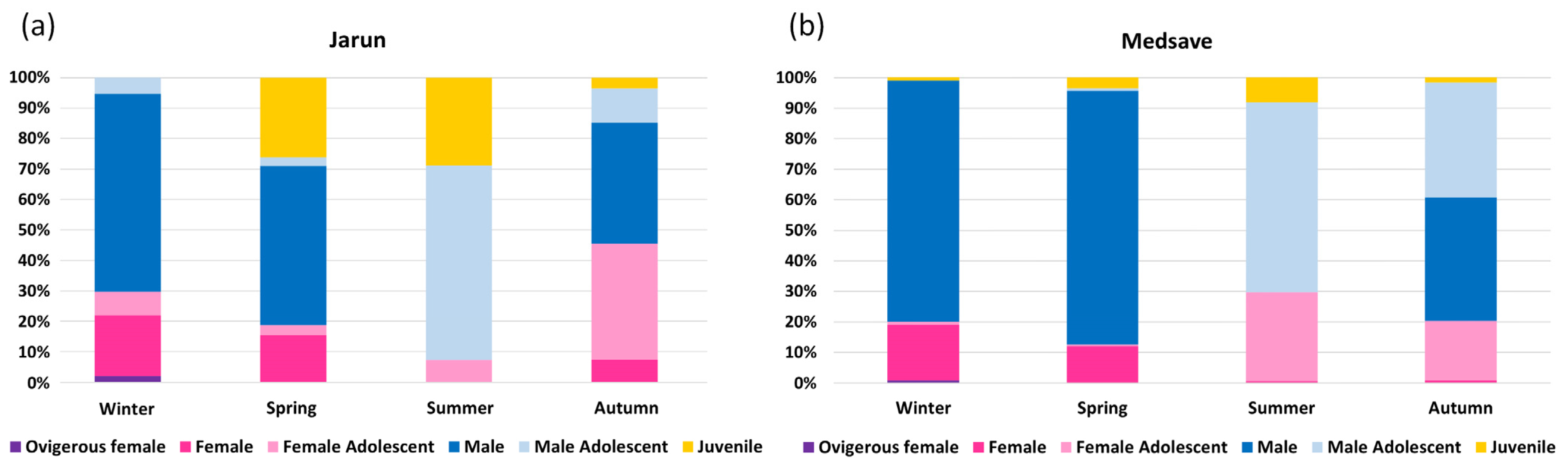
3.1. Population Structure

A total of 616 specimens (adults and adolescents) of S. ambulans (185 female, 431 male) from the Jarun study site and 892 (196 female, 696 male) from the Medsave study site were analysed (Table 1). A total of 123 juveniles were sampled at the Jarun site and 38 juveniles were sampled at the Medsave site. At the Jarun sampling site, the most distinct population peaks occurred in the spring (April 2019) and autumn (October 2019). At the Medsave sampling site, the highest population abundances were observed in summer (July 2019) and autumn (October 2019) (Table 1). There was no statistically significant difference in the S. ambulans abundances between the two sampling sites (p = 0.221).
The frequency distribution of the different life stages is shown in Figure 3. At the Jarun site, the peak of juveniles represented 26% and 29% of the population in spring and summer, respectively. The highest peak of adolescents was in the summer and accounted for 71% of the population. The two peaks of adults were in winter and spring and accounted for 87% and 67% of the population, respectively. At the Medsave site, an increase in juveniles was observed in the summer. The highest peak of adolescents was in the summer and accounted for 91% of the population. Adults accounted for more than 90% of the population in winter and summer. Intersexuality was not detected in any of the amphipod populations in this study.
The statistical comparison of TBL between study sites showed that the TBL of females and males in winter and spring and that of males in autumn were significantly higher at the Medsave site compared to the Jarun site (Table 1 and Table 2). A significantly higher TBL of adolescent males was found only in autumn at the Jarun site (Mann–Whitney U test, level of significance p < 0.05). A comparison between TBLs of males at both study sites revealed no statistically significant difference, whereas females at the Jarun site had significantly higher TBLs compared with females at the Medsave site (p < 0.001). During all four seasons, females had significantly higher TBL than males at both study sites (p < 0.001). Significant seasonal differences were found at the Medsave site for females, female adolescents, males, and male adolescents, whereas at the Jarun site differences were found for females, female adolescents, males, and juveniles (Kruskal–Wallis One Way Analysis of Variance on Ranks, p < 0.05).

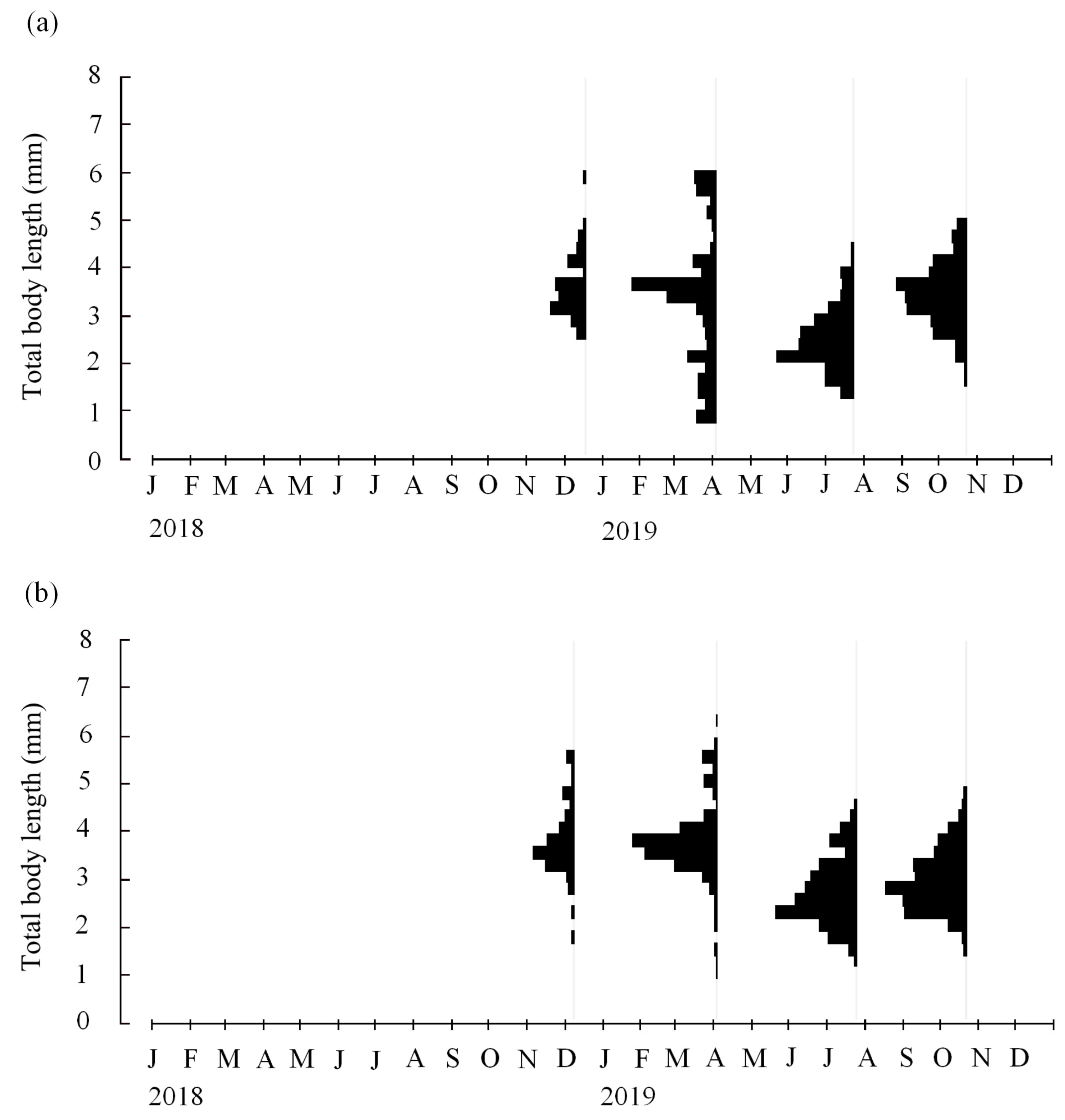
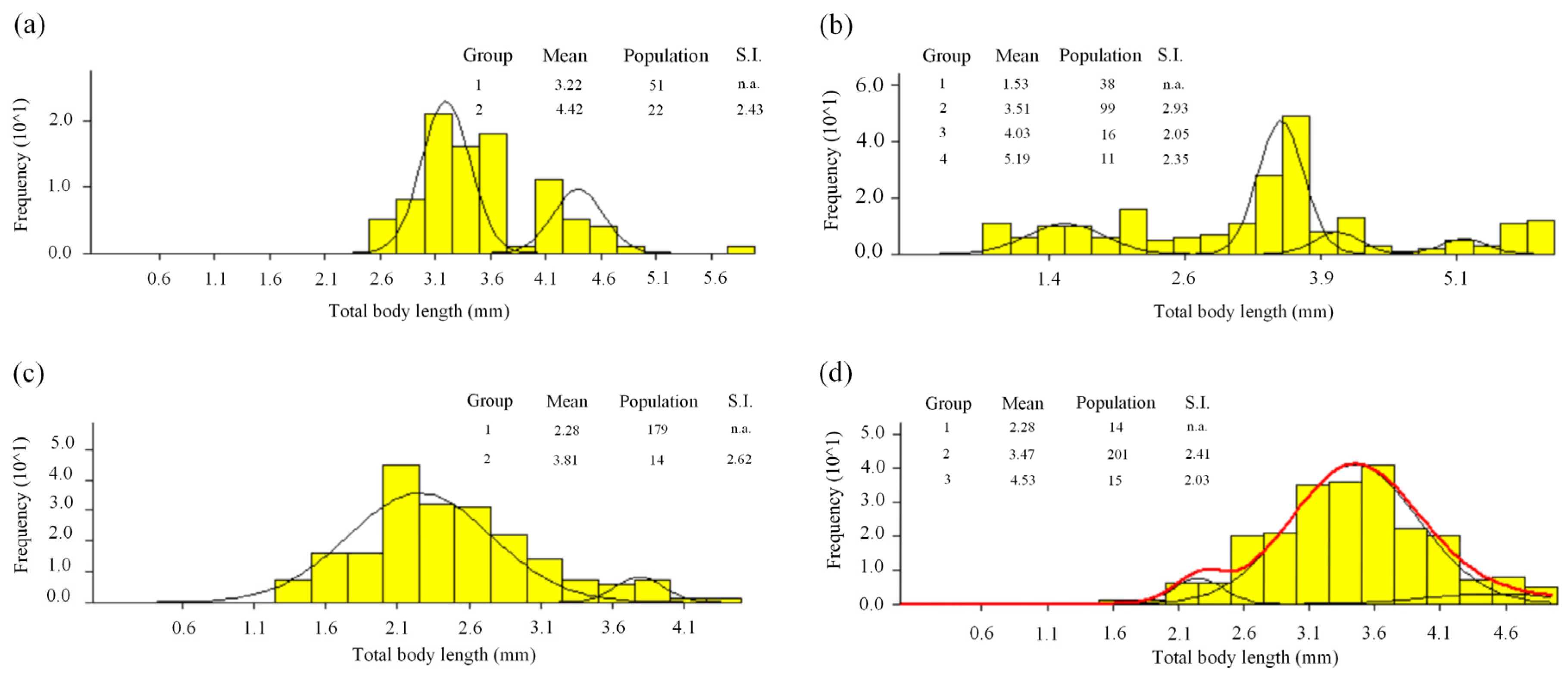
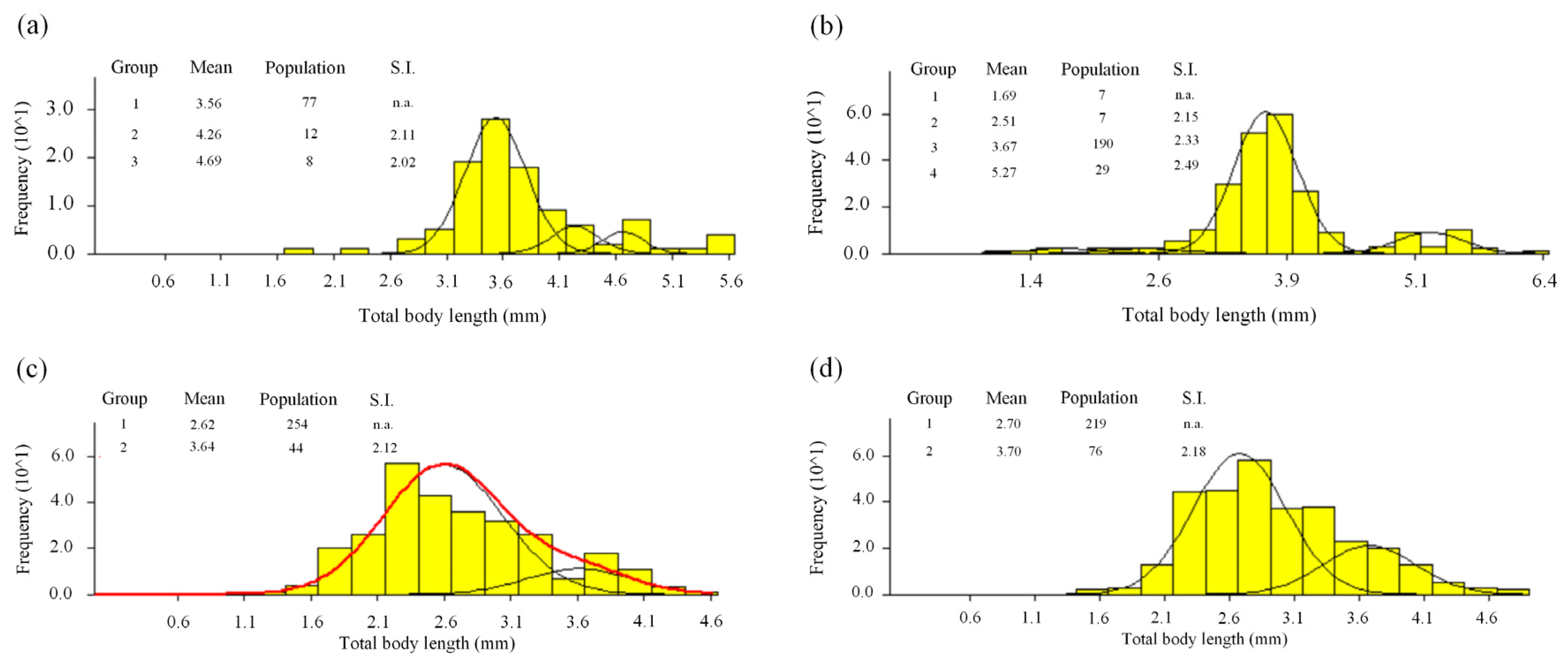
3.2. Length-Frequency Analysis

For the length-frequency analysis, female adolescents were pooled with adult females and male adolescents with adult males. The frequency distribution of female TBL ranged from 2.80 to 6.00 mm (mean female TBL = 4.23 mm; SD = 0.87) in the Jarun study site, whereas it ranged from 2.10 to 6.38 mm (mean female TBL = 3.84 mm; SD = 1.04) in the Medsave study site in all seasons (Table 1 and Table 2). Male TBL ranged from 1.75 to 4.50 mm (mean male TBL = 3.26 mm; SD = 0.56) in the Jarun study site, and from 1.80 to 5.00 mm (mean male TBL = 3.31 mm; SD = 0.64) in Medsave (Table 1 and Table 2). At both study sites and in all four seasons, females had a greater size range (2.10–6.38) than males (1.75–5.00). At the Jarun site, females had a wider range of size classes in winter, spring, and autumn. Males had a wider range of size classes during the summer (Figure 4a). At the Medsave site, females had a wider range of size classes in spring, whereas males had a wider range of size classes in winter, summer, and autumn (Figure 4b).
The highest frequencies of female TBL were between 3.50 and 3.80 mm in Jarun in autumn and between 2.60 and 2.80 mm, and between 3.10 and 3.30 mm in Medsave in summer, while the highest TBL frequencies of males were recorded between 3.50 and 3.80 mm in Jarun in spring and between 2.50 and 2.80 mm in Medsave in autumn. Overall, females were more abundant in the smaller TBL size classes, while males were more abundant in the larger TBL size classes. The values of sex ratio on the Jarun study site were significantly different from 1:1 in most seasons (χ2-test, p < 0.05), and they were male based, except in autumn, when the population was in equilibrium (Table 1). The sex ratio was significantly different from the expected equilibrium in all seasons in the Medsave study site, always favouring males (Table 1 and Table 2). The sex ratio was exceptionally biased towards males in spring at Medsave and in summer at the Jarun site. The breeding period could not be estimated because ovigerous females were recorded in extremely low numbers (only three specimens in December).
The estimated parameters of VBGFs for Jarun and Medsave sites differed between sexes (Table 3). For females, K and φ′ were higher at the Jarun site than for females at the Medsave site, whereas L and tmax were higher at the Medsave site. For males, L and tmax were higher at the Jarun site than for males at the Medsave site, while K and φ′ were higher at the Medsave site. At the Jarun study site, females had higher values of K, L, and φ′ than males, while males had higher tmax compared to females. At the Medsave study site, females had higher L and tmax, while males had higher K and φ′ compared to females. The estimated growth parameters of different species of Amphipoda obtained from other studies are compared in Table 4.

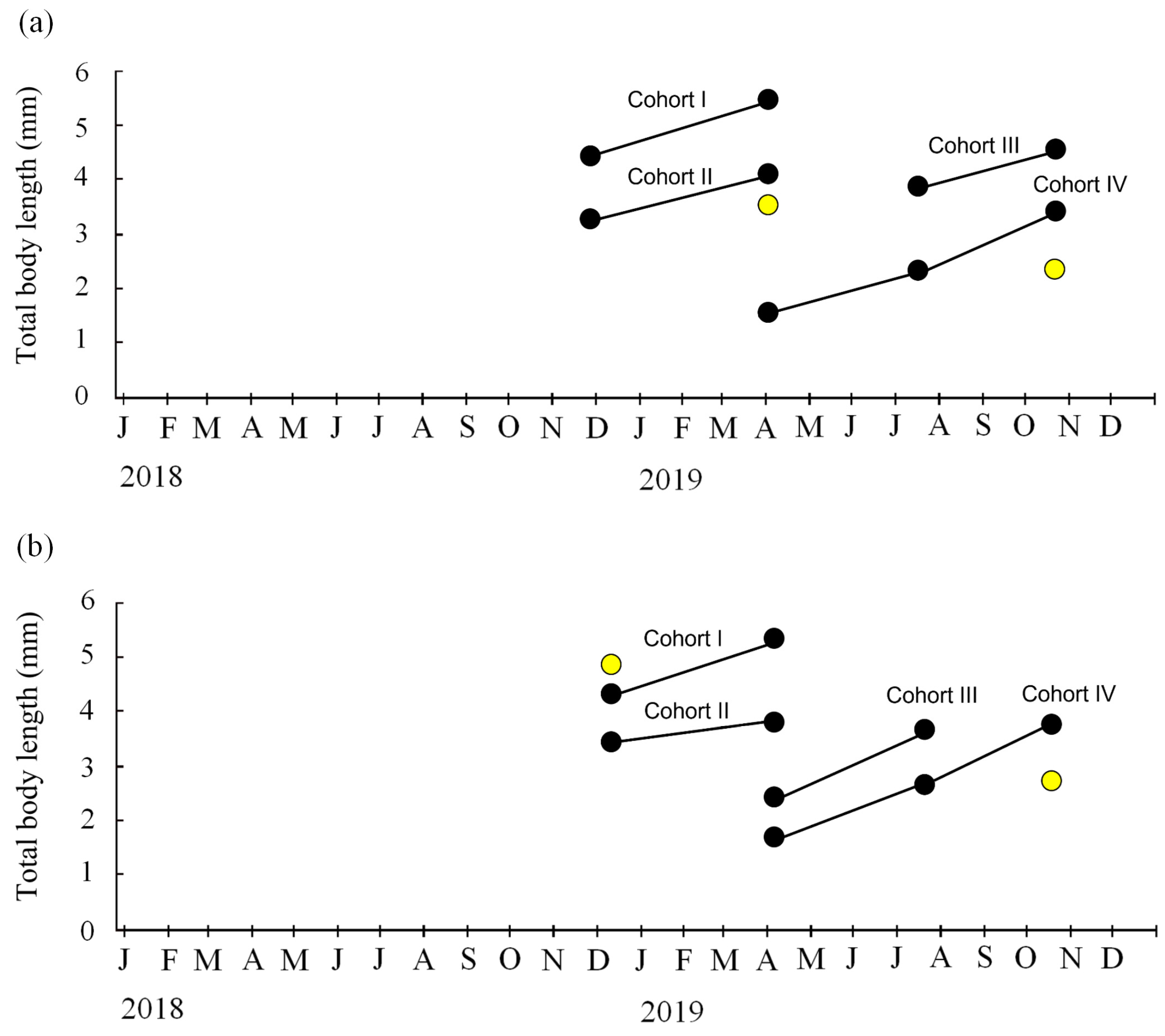
3.3. Cohorts and Growth

The four cohorts of S. ambulans were identified during one year at each study site (Jarun and Medsave) based on length-frequency distribution and confirmed with the Bhattacharya method (Figure 5, Figure 6 and Figure 7). At the Jarun study site, relatively large overwintering adults (Cohort I and Cohort II) were detected from December 2018 to late April 2019 (Figure 5 and Figure 7a). Adults of Cohort III were detected from July to October 2019, and adults of Cohort IV from April to October 2019. The largest amphipods disappeared from the population after the spring season (Figure 7a). The largest adult males and females were found in the population in April 2019, with a mean total body length of 4.40 mm and 6.00 mm, respectively.
At the Medsave study site, amphipods at the upper level consisted of two parallel cohorts (Cohorts I and II) from December 2018 to April 2019 (Figure 6 and Figure 7b). During the spring and early summer (April to July 2019), a new cohort, Cohort III, appeared in the population (Figure 7b). Cohort IV increased in size and number from April to October 2019. Juveniles from Cohort III and Cohort IV probably appeared in the population in the early summer of 2018 and autumn 2018, respectively. The largest adult males were detected in the population in December 2018, with a mean total body length of 4.75 mm, and disappeared from the population by summer 2019. The largest adult females were recorded in April 2019, with a mean total body length of 5.70 mm, and disappeared from the population during the summer. The longest cohort life span of both populations was eight months (Figure 7a,b).

3.4. Mortality

In the present study, amphipod mortality was calculated for the entire population of S. ambulans (Table 5). The total mortality coefficient (Z) was estimated from the slope value of the length-converted catch curve, separately for the combined sex, females, and males of the Jarun and Medsave populations. The estimated total mortality (Z) for separate sexes had higher values for males than females at both sampling sites. The estimated natural mortality (M) was higher for males compared to females at the Medsave site and higher for females at the Jarun site. The highest value of natural mortality (2.65 year−1) and total mortality (4.60 year−1) was calculated for males at the Medsave and the Jarun study sites, respectively. A comparison of length-converted catch curves showed that M was higher for females at the Jarun site, and for males at the Medsave site. Total mortality was higher for both females and males at the Jarun site than at the Medsave site. The natural mortality of the Jarun population (M = 2.98 year−1, combined sex) corresponded to about 86% of Z, revealing the low propagation of this species in the HZ of the Sava River at the Jarun study site. The natural mortality of the Medsave population (M = 1.30 year−1, combined sex) corresponded to about 62% of Z, revealing the extremely low repopulation of the species in the HZ in this part of the Sava River. The natural mortality to growth factor (M/K) ratio was highest at the Medsave site for females and lowest at the Jarun site for the combined sex (males and females combined).
Both the M/K ratio and the Z/K ratio were higher for females than for males at the Medsave site, and for males at the Jarun site.

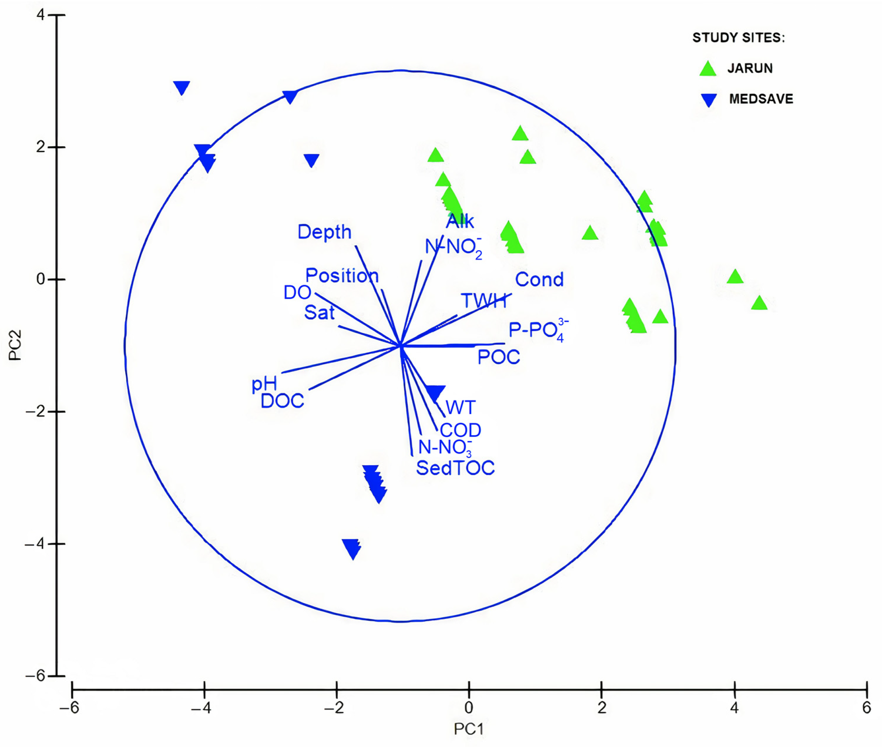
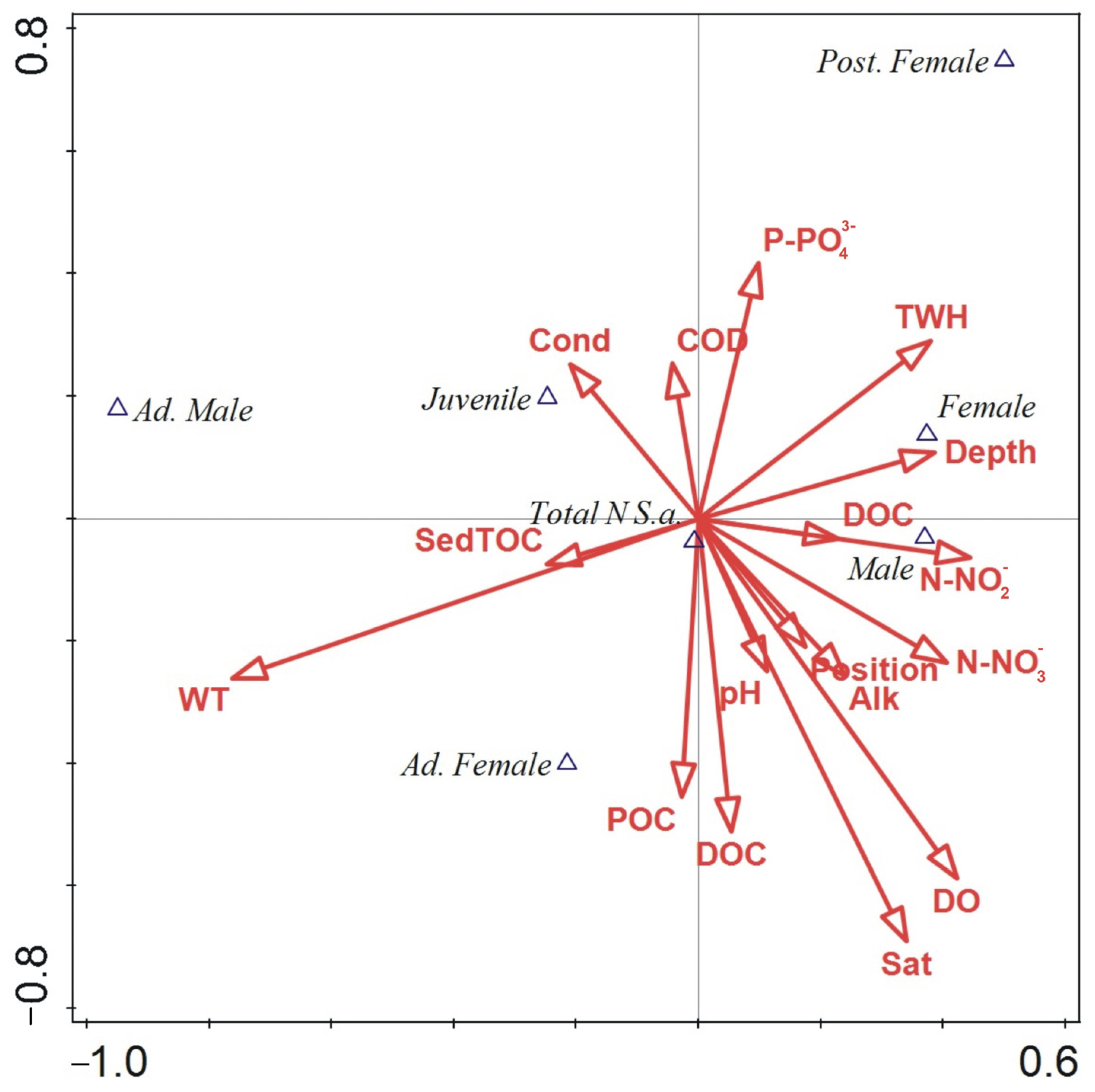
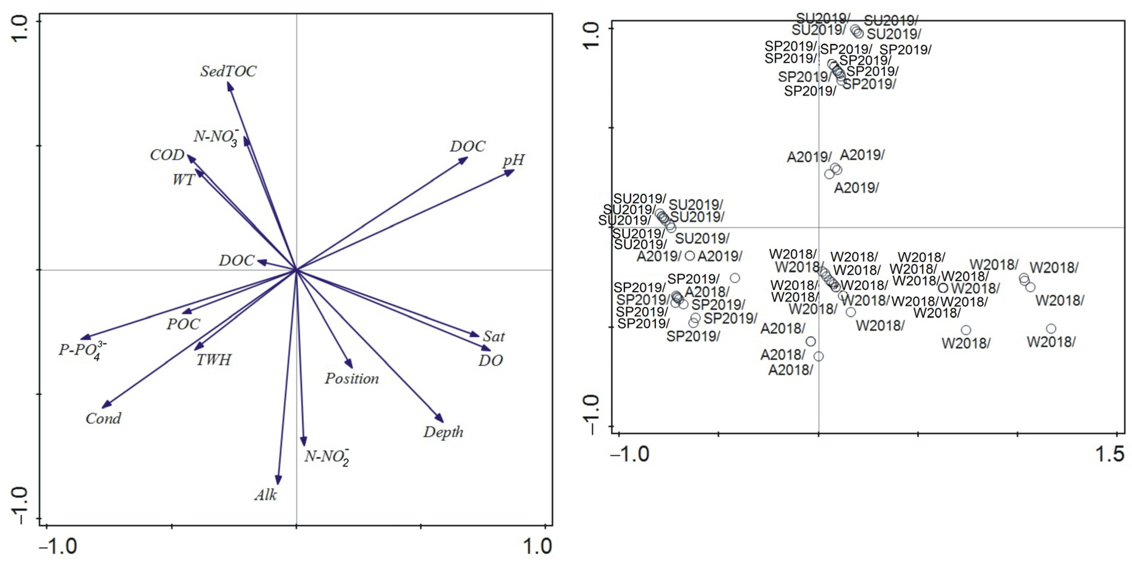
3.5. Relationship between Environmental Parameters and Gender/Ontogeny Classes’ Abundance

A previous paper already presented the detailed environmental parameters [47]. In this research, new parameters (sampling depth and position of the Bou-Rouch pump) were added that were the key factors in the analysis of S. ambulans populations in the HZ, and they were all combined using the new types of analyses (PCA and CCA). A seasonal temperature gradient was observed in the HZ of the Sava River, ranging from 10.4 °C in winter (December) to 23.3 °C in summer (July) at the Medsave site and from 12.7 °C in winter (December) to 16.5 °C in summer (July) at the Jarun site (Table 6).
The PCA analysis indicated that the first two axes of the PCA explained 48.9% of the variance among samples (PC1 = 27.2% and PC2 = 21.7%) and revealed slight differences between environmental parameters on the study sites, mainly due to Alk, Cond, depth, DO, DOC, pH, and P-PO43−. The pH (eigenvalue = −0.432) and Cond (eigenvalue = 0.406) presented the strongest correlations in PC1, while Alk (eigenvalue = 0.404) and N-NO3 (eigenvalue = −0.323) were the most important variables in explaining the PC2 (Table 7, Figure 8).
The influence of environmental parameters on the amphipod analysed classes was investigated using CCA, which showed that overall, different classes of S. ambulans (gender (male and female) and ontogeny (adult, adolescent and juvenile)) were associated differentially with environmental variables. All classified categories were distributed along the four axes of the CCA. The first axis had an eigenvalue of 0.3 and the second axis had an eigenvalue of 0.1, with both axes exhibiting gender/ontogeny–environment correlations of 0.9. The Monte Carlo test was significant (test of significance of all canonical axes: trace = 0.56; F-ratio = 9.9; p < 0.005) and cumulatively, axes 1 and 2 accounted for 77.6% of the total variance, with correlations between the density of S. ambulans classes (gender and ontogeny) and environmental variables of 0.973 (axis 1) and 0.894 (axis 2). According to the correlation coefficients, DO, DOC, position, and Sat had a high positive correlation to the first CCA axis, while WT and POC were negatively correlated. The depth of samples, TWH, and concentration of P-PO43− were positively correlated with the second CCA axis, while Cond and COD were negatively correlated. Adult males were primarily associated with the concentration of N-NO2, while adult females were associated preferably with the depth of samples and TWH. The juveniles were associated with Cond, while adolescent females were primarily associated with POC (Figure 9).
The ordination of the samples showed that they tended to cluster following the seasons, revealing a temporal gradient according to the CCA axes (Figure 10). Winter samples (W) with higher DO and Sat and pH value clustered on the positive side of the first CCA axis. Spring samples (SP) with high Cond and P-PO43− clustered on the negative side of the first CCA axis. Summer samples (SU) with high Cond and the lowest concentration of DO clustered mainly on the negative side of the second CCA axis. Autumn samples (A) were characterised with the highest TOC concentration and clustered on the negative side of the first CCA axis and the positive side of the second CCA axis (Figure 10).

4. Discussion

4.1. Life Cycle

The life cycle of S. ambulans has previously been studied in populations from Romania, Poland, and Germany, respectively [7,11,33]. These are the only data on the life history of S. ambulans in the literature. The population structure of S. ambulans from Poland and Romania differed from the population in the Sava River. In our study, the recruitment of the new generation began in April, while in the population in Romania it began in May and in Poland it began later, in June [7,11]. Thus, the population in Romania became bimodal (consisting of adults and juveniles) in May, the population in Poland became bimodal in July and August, and the population in the Sava River became bimodal in April. In all populations (Romania, Poland and Croatia), the parent generation had disappeared in summer (June, July, and August). The juveniles that appeared in Poland in summer grew to sexual maturity in the following spring. It was concluded that S. ambulans in Romania have an annual univoltine (one generation per year) semelparous (single-breeding) life cycle [7]. In the study from Poland, it was suggested that the life cycle of S. ambulans is univoltine and iteroparous (females produce only a few broods in their lifetime) [11]. It has been shown that gammarids living in stable water temperatures with a groundwater supply are iteroparous and breed continuously [121]. Our study showed that the life cycle of S. ambulans may be univoltine, with the extremely low number of ovigerous females found only in December (three specimens). Such differences in life cycle between S. ambulans populations at different latitudes or altitudes (Poland, Romania, and Croatia) may be due to seasonal variations (temperature regime, different longevity of unfavourable conditions) [7]. In Poland, the water temperature ranged from 0.8 °C in January to 18.8 °C in July. In Romania, the temperature range was the highest, with water temperature ranging from 2.5 °C in December to 24 °C in July and August. In our study, the temperature ranged from 10.4 °C in December to 23.3 °C in July (Table 6).
Thus, different temperature minima and maxima may result in different recruitment periods among these S. ambulans populations. This was particularly evident in the later reproduction and recruitment in the population from Poland, where temperatures were lowest and the latitude highest. Depending on whether they live at high or low latitudes, gammarids are semelparous or iteroparous, respectively [56]. In the amphipods Monocorophium insidiosum (Crawford, 1937) and Corophium multisetosum Stock, 1952, the lifespan and number of generations were also affected by latitude [122,123]. The number of cohorts of the same crustacean species, Neomysis americana (S.I. Smith, 1873), was shown to be more strongly related to temperature regime (the higher number of cohorts was recorded at higher temperatures) and to a lesser extent to latitude [84]. In addition, the S. ambulans populations from Poland and Romania were epigean—found in a shallow pond and flowing rivers in lowlands, respectively. On the other hand, the S. ambulans population in Croatia was hypogean—inhabiting the river’s HZ (GWCE). Thus, the different habitats could also be the reason for the differences in the life cycle of S. ambulans.
Data on the sex ratio of S. ambulans indicate that males were more abundant than females in all seasons, while the opposite was found in populations from Poland and Romania [7,11]. The overall sex ratio in Poland and Romania was 1:0.4 (634 females and 247 males in Poland), while in our study it was 0.4:1 (185 females and 431 males) at the Jarun site and 0.3:1 (196 females and 696 males) at the Medsave site. Compared to other amphipod species, such as Crangonyx pseudogracilis Bousfield, 1958 and Waldeckia obesa (Chevreux, 1906), the sex ratio was in favour of females [66,83], while the proportion of males was higher than that of females in Nototropis minikoi (A.O. Walker, 1905) [82]. Several factors may influence the changes in sex ratio, such as different mortality rates between males and females [88,124,125,126], different longevity or differences in the minimum size at which secondary sexual characteristics appear [125,127]. One of the reasons for the differences in sex ratios in amphipods could be chemicals from agriculture and from untreated sewage [83,128]. In our study, the male-biased ratio could be due to the females (which are larger than males) being more vulnerable to the lower oxygen concentration in the HZ and requiring larger amounts of food, and therefore inhabiting the shallower part of the HZ with more oxygen and food. Moreover, it is possible that the male-biased ratio is due to the fact that males require a greater number of moults to become sexually mature. Synurella ambulans has a longer life cycle compared to other epigean amphipods [83,129], resulting in more extended maturation and growth. It has been previously shown that amphipods disappear from the population after mating (males) or after the release of the brood (females) [130]. Thus, males of S. ambulans remain in the population in high numbers until females are sexually mature and until they have completed breeding.
The observed TBL values of S. ambulans were similar to the TBL values reported in previous studies [11]. The maximum size of males (4.7 mm) was comparable to the maximum size of 4.8 mm recorded in our study, whereas the maximum size of females (7.0 mm) was higher than in our study (6.4 mm). The size difference between females and males might be related to mating behaviour, since there is no pre-copula pairing (where males are larger than females) in S. ambulans [7]. In our study, the maximum TBL of females and males were higher at the Medsave site than at the Jarun site. It was suggested that the significant differences in the length of individuals of Dikerogammarus haemobaphes (Eichwald, 1841) (Amphipoda) inhabiting two sites with different hydrological characteristics could be due to different hydrological conditions and different predation pressures [81]. In our study, the water levels and discharges of the Sava River were similar at the two sampling sites. Another important factor influencing the differences in maximum TBL values between sampling sites could be nutrient level. DOC and TOC concentrations were higher at the Medsave site than at the Jarun site, which could result in higher maximum TBL values. Similarly, it was shown that the largest size of Emerita analoga (Stimpson, 1857) females was associated with food availability [131].
Regarding seasonality, the mean TBL of females and males at both sites was lowest in summer because the population consisted only of juveniles and adolescents. When we observed only sexually mature individuals, the lowest mean TBL was in autumn for most age groups (females at the Medsave site and males at the Medsave and Jarun sites). The opposite pattern was observed in the study on adult individuals of the amphipod Dikerogammarus haemobaphes, who had the lowest size in summer and the highest size in autumn [81].

4.2. Growth and Mortality

The analysis of growth parameters revealed that both males and females had different growth rates depending on location. Recent studies have shown that population density can affect crustacean growth, as they were negatively correlated [86,132,133]. However, in our study, no significant correlation was found between amphipod abundance (n of individuals in 50 L) and mean animal size (Pearson coefficient rfemale = −0.425, rmale = −0.307; p > 0.05). The estimated growth parameters (K and φ′) for the two populations (Jarun and Medsave) showed that females grew faster than males at the Jarun site, while the opposite was observed at the Medsave site. The females of Crangonyx richmondensis Ellis, 1941, C. pseudogracilis (both belonging to the same family of Crangonyctidae as S. ambulans) and Dikerogammarus villosus (Sowinsky, 1894) had a higher growth rate than males [83,134,135]. In contrast, a higher growth rate was recorded for males than females in the Antarctic amphipod W. obesa [66].
In the populations of S. ambulans from the Jarun and Medsave site, four cohorts were identified during one year, which is an extremely low number of generations in comparison to small surface river dwelling amphipods such as Echinogammarus cari (S. Karaman, 1931), with as many as 12 cohorts per year [136]. At the Jarun study site, the large overwintering adults belonging to Cohort I and Cohort II would produce the new offspring, which would appear in the population at the beginning of the next year (2020). Since adults of Cohort III and of Cohort IV were detected in the population in spring, summer, and autumn 2019, juveniles from Cohort III and Cohort IV likely appeared in the population in early summer 2018 and autumn 2018, respectively. At the Medsave study site, Cohorts I and II would produce new offspring, which would appear in the population at the beginning of the next year (2020). Based on the observations of Cohort IV, which gradually increased in size and number from April to October 2019, it likely reached the sexually mature phase in winter 2020. The growth of the third cohort at the Jarun study site was faster at lower temperatures than at the Medsave study site, with higher average water temperatures in the HZ during the spring and summer (Table 6). The present research showed that the individual cohort life span in S. ambulans in the HZ of the Sava River could be more than 12 months long, which was more similar to the surface freshwater amphipod E. cari adapted to cold water streams, with a cohort life span of 6 to 12 months [136].
The influence of environmental factors (e.g., hydrological conditions, sediment type, temperature, food availability, water mass movements in the sea) on crustacean growth parameters has been reported by several authors [79,85,123,127,137,138,139,140]. A comparison of the estimated growth parameters of VBGF with other amphipod species revealed similar K values of S. ambulans with the polar species W. obesa from Antarctica, Gammarus wilkitzkii Birula, 1897 from the Arctic, and with N. minikoi from the Caribbean Sea (Table 4). This generally lower growth rate of S. ambulans compared to another amphipod, Pseudorchestoidea brasiliensis (Dana, 1853), may be related to the lower metabolic rate and oxygen consumption regularly found in hypogean amphipods [141,142]. Meagre oxygen consumption rates have also been measured in polar amphipods [143]. This supports the suggestion that a lower growth rate is related to lower oxygen consumption in species living in Arctic regions under sea ice [120].
Considering the population types defined by Schwamborn [144] (“type A” and “type B”) and using the “Lmax approach” (maximum length approach, i.e., the largest organism in the sample) [145], we analysed the two populations in the Sava River. At the Medsave site, L (7.20) for females was greater than Lmax (6.38), and L (6.30) for females was greater than Lmax (6.00) at the Jarun site. This points to a “Type B” population characterised by slow growth and a very high Z/K ratio [144], but not a typical one, since Lmax was not far below L.
The total mortality rate of S. ambulans differed between males and females at both sites, with males exhibiting a higher mortality rate. High daily water level amplitudes are the first hypothesis that may explain the differences between mortality rates. Adult males (individuals with lower TBL) may remain in the upper layer of the sediment, while adult females (individuals with higher TBL) are more profound. In this way, males may remain without water and nutrients for a period of time, which could eventually lead to higher mortality. It was suggested that small individuals (juveniles and males) of the anomuran crab Emerita brasiliensis Schmitt, 1935 that remain near the substrate surface are more exposed to tide changes compared to larger females [87]. Consequently, this stratification by sex and size may lead to size-dependent mortality. Another hypothesis is that males are more vulnerable to predation because they need to find females to mate with [146]. The higher total mortality rates of females and males at the Jarun site compared to the Medsave site could be explained by lower food availability, as DOC and TOC concentrations were lower at the Jarun site (Table 6). The importance of food has been documented as one of the factors explaining the mortality rate of E. brasiliensis [87].
The natural mortality of amphipods can be caused by predation, disease, age, and environmental factors [93,147,148]. The previous study confirmed the high mortality rate of amphipods in the HZ under extreme hypoxic conditions [148]. This could be for the same reason as the high natural mortality of males (2.65 year−1) in the HZ of the Medsave study site, due to strong water level fluctuations, and very often a low flow velocity. However, those conditions affected the Jarun population less, since males had lower natural mortality compared to males at Medsave. In addition, the Medsave and Jarun populations were under the extreme influence of water level fluctuations caused by hydroelectric power plants (HEPPs) in Slovenia, resulting in daily changing rewetting and drying fluctuations.
The growth–mortality continuum was introduced for benthic invertebrates, where ΔZ/k is a measure of relative predation pressure [149]. Calculated ΔZ/k values for S. ambulans were positive for males (0.56) and females (0.19) at the Jarun site and for females (0.09) at the Medsave site, suggesting higher than average predation pressure. It was suggested that S. ambulans may be preyed upon by the larger amphipods [7]. However, in the Sava River, only turbellarians were found in the samples from the HZ as potential predators of S. ambulans.
Differences in populations and species longevity in crustaceans could be influenced by variations in growth rate, mortality, and local environmental conditions such as temperature, concentration of organic matter, and oxygen [83,150,151,152]. The lifespan of amphipods can vary from a few months to over 10 years [56]. Species with long life spans usually live under harsh environmental conditions (e.g., low temperatures, high seasonality of food availability) [120,153]. S. ambulans showed high longevity, similar to the amphipods W. obesa (>5 years) [66] and G. wilkitzkii (5 years) [120]. S. ambulans had a higher longevity compared to other amphipod species that live in temperate waters, such as Echinogammarus marinus (Leach, 1816) and C. pseudogracilis, whose longevity can be as long as 1 and 2 years, respectively [83,129]. The higher longevity of females at the Medsave site compared to females at the Jarun site may be related to the lower total and natural mortality of females at Medsave. However, this pattern could not be explained in males, which had higher longevity and total mortality at the Jarun site but lower natural mortality than at Medsave. The influence of higher mortality rate on shorter life span was shown in E. brasiliensis [127].

4.3. Environmental Factors and Life History Traits of S. ambulans

Several environmental factors in the Sava River were recorded to have a substantial impact on population dynamic and general life history traits of the species S. ambulans. Temperature, as a key environmental factor, has a great influence on the growth and number of moults of crustaceans [60,154], with the growing rate related to high temperature values. Species from cold climates have a longer life span and larger body size, while species from warm climates have a shorter life span and reach smaller body sizes [56]. In addition, temperature has been shown to affect the macroinvertebrate community structure [155,156]. Synurella ambulans is a euryoecious organism (adapted to different habitats) [9] that can tolerate a wider range of physico-chemical parameters, including temperature, although it belongs to the cold stenothermal group of amphipods [13], with some races highly adapted to stable subterranean environments [20]. The higher maximum water temperature at the Medsave study site (23.3 °C) could lead to a faster growth rate of males at this site, compared to the Jarun population with a narrower temperature range and lower maximum water temperature values (16.5 °C) (Table 6). Optimal water temperature is important for crustacean longevity [83]. In GWCE, such as the HZ, the optimal water temperature is equal to the mean annual air temperature. Accordingly, the optimal physiological temperature of S. ambulans in the Sava River plain is 11.6 °C (for the period from 1862 to 2016) [157]. According to the Climate Atlas of SFRY (for 1931–1960) [158], the mean annual temperature was 10–11 °C and, according to Zaninović et al. [159], 11–12 °C. Environmental temperature may affect the duration of the reproductive period; for example, in the isopod Excirolana braziliensis Richardson, 1912, reproduction was seasonal and may have been interrupted due to temperature fluctuations in the sea [160]. In our study, reproduction was also seasonal, as ovigerous females occurred only in winter. This can be justified by the claim that S. ambulans, as a representative of the family Crangonyctidae, is in fact a cold-water species [13]. The number of recruitment events that occurred in spring and summer did not differ between Jarun and Medsave populations. The temporal scale (seasonal sampling) used in this study could affect the interpretation of growth results, as S. ambulans populations could change over shorter periods of time. Therefore, a more detailed (monthly) study with longer data series is needed to provide a more accurate estimate of cohort numbers and growth parameters. However, due to the decreasing number of gravel bars along the Sava River and the potential vulnerability of the species to extinction, we believe that such an intensive sampling campaign would not be acceptable. It was shown that populations of E. braziliensis are influenced by daily changes [161]. Therefore, short-term hydrological variations, such as abrupt daily changes in water level amplitudes of the Sava River, may also influence changes in the population structure.
Our results highlighted that S. ambulans are distributed unevenly in the HZ throughout the year based on the influence of various environmental factors on gender and ontogeny classes. Among crucial environmental factors in the HZ were food amount belonging to the community and abundance balancing variables where higher nitrate promoted the decomposition of leaf litter via stimulated detritivore feeding activities [162], which also includes S. ambulans. Determined relations in distribution patterns of different genders and groups of organisms according to ontogeny and environmental parameters in our analysis were confirmed through the oscillation of organic matter with the depth of the samples. Moreover, part of the organic matter may remain below the streambed during flooding or sediment movements at higher water discharge [162], which also occurs in the investigated study sites due to the large influence of the HEPP in the upstream parts of the Sava River. The investigated species S. ambulans, like most hyporheic invertebrate communities, responds to the seasonal flow recession, which was documented even for macroinvertebrates entering the HZ in a groundwater-dominated stream [163]. CCA analysis showed strong relations with temperature and oxygen as the most important environmental parameters in the HZ, influencing growth and development in both gender and ontogenetic stages in S. ambulans. Both environmental factors have been shown as regulation parameters for growth and development in crustaceans [60,83]. General suboptimal environmental conditions in the HZ of the Sava River during the summer (higher temperature values and lower oxygen, Table 6) due to lower hyporheic flow could be the reason for the negative relation with the abundance of lower ontogenetic classes (adolescent males and females) as more sensitive to warming and hypoxic conditions.

4.4. Advantages and Limitations of Length-Based Methods for Amphipod Studies

Size-frequency growth models are an important source of information on age and longevity in crustaceans because they are powerful, cheap, easy to apply, and require very few resources [139,164]. Although other, more accurate methods for age determination exist (e.g., tagging and recapture, lipofuscin-based ageing, radiometric ageing), these size-frequency-related growth models are still extremely relevant, especially for many small shrimps [165]. Size-frequency growth models have been shown to be more reliable for short-lived species (e.g., mysids such as the opossum shrimp N. americana (10 months)) than for long-lived species (e.g., decapods such as the crayfish Pacifastacus leniusculus (Dana, 1852) (16.7 years)) [91,139,166]. However, such growth analyses have limitations and must be used and interpreted with caution [164]. The need for additional data or assumptions is a common limitation of length-frequency based models, and alternative conclusions are possible depending on them [166]. In addition, it has been shown that methods used to fix or constrain L a priori can introduce bias in their L estimates [144]. Methods used for the unconstrained search for optimal combinations of growth parameters, such as Response Surface Analysis, do not provide 95% confidence intervals for estimates (e.g., K and L) [165]. Current length-based methods were critically evaluated and a new pseudo-R² index for the goodness of fit of von Bertalanffy growth models (a low index implies a “poor” dataset and small sample size) was proposed [165]. This new bootstrap-based method offers a promising new direction for length-based analyses of growth and mortality in natural populations, especially due to its high reproducibility and accuracy.

5. Conclusions

The environmental adaptation of S. ambulans to the hyporheic interstitial zone in the present study could originate from eco-physiological adaptations of the species to better cope with the habitat intermittency (huge daily rise and fall of the water level in the Sava River coming from the upstream parts in Slovenia due to the influence of HEPPs), huge oscillations of the water current, and consequently fluctuating environmental parameters and steep abiotic and biotic (life history) gradients. Another factor influencing the adaptation capacity could be connected to the directional selection of life in subterranean environments where energy demand is lower relative to surface habitats.
Thanks to the present study, we noticed that S. ambulans is a very active burrower in the HZ and, as such, belongs to the key bioengineers unclogging hyporheic interstitial space because the spatial and functional suitability of the HZ is impaired when the interstitial pore space becomes clogged. Thanks to burrowing, the activity of the species plays a vital role in the vertical connection and exchange between free-flowing surface water, pore water of the HZ, and groundwater (upwelling and downwelling), and thus we can declare the species to be a guard of the HZ and a sentinel of climate change.
In our study, intrinsic (result of aging) and extrinsic (environmental caused) factors influenced the natural mortality rates in S. ambulans populations, increasing in the environmental conditions with expected higher metabolic rates (higher temperature, lower oxygen), and lowering the longevity of populations. The size of females reaching sexual maturity changes seasonally and mainly depends on water temperature. The shallow hyporheic interstitial zone may only represent a refuge for S. ambulans, which means the species does not complete its entire life cycle in this environment because it uses the hyporheic interstitial as a spawning habitat, which was confirmed by the presence of juveniles, but not as a nursery place due to the lack of ovigerous females. A fine-scale life history trait analysis covering at least three years of observations is needed for a complete overview of cohorts.
The species S. ambulans acts as an essential link in the transfer of matter and energy in the hyporheic interstitial zone, and knowledge of its population dynamic and life history traits is crucial for the conservation strategy of the species and its environment. Due to the ecological relevance of the species to the hyporheic ecosystem, it is important to protect the gravel bars it inhabits along the Sava River and European rivers in general. Our results may help future researchers to conserve the GWCE as a whole, especially regarding the conservation purposes of S. ambulans as a species inhabiting the vulnerable HZ of the Sava River.

Author Contributions

Conceptualization, S.G. and Z.R.; methodology, S.G. and Z.R.; formal analysis, S.G. and Z.R.; investigation, S.G., Z.R., M.E., M.S.P. and J.D.; resources, S.G., Z.R. and M.E.; data curation, S.G. and Z.R.; writing—original draft preparation, S.G. and Z.R.; writing—review and editing, M.E., M.S.P., J.D. and M.C.; visualization, S.G. and Z.R.; supervision, S.G.; project administration, S.G., M.E. and M.C.; funding acquisition, M.E. and M.C. All authors have read and agreed to the published version of the manuscript.

Funding

This research was funded by the European Regional Development Fund, project KK.01.1.1.07.0023: “Qualitative and Quantitative Protein Analysis in Medicine and Biotechnology Industry” (Qua/Qua Protein), and by the Croatian Science Foundation, project IP-2014-09-4255: “Accumulation, subcellular mapping and effects of trace metals in aquatic organisms” (AQ-UAMAPMET).

Data Availability Statement

The data presented in this study are available on request from the corresponding author.

Acknowledgments

The authors sincerely thank Ivica Barač for his great help in the field work during the sampling campaigns and Neda Vdović for PSD measurements.

Conflicts of Interest

The authors declare no conflict of interest.

References

  1. Arfianti, T.; Wilson, S.; Costello, M.J. Progress in the Discovery of Amphipod Crustaceans. PeerJ 2018, 6, e5187. [Google Scholar] [CrossRef]
  2. Benito, J.B.; Porter, M.L.; Niemiller, M.L. Comparative Mitogenomic Analysis of Subterranean and Surface Amphipods (Crustacea, Amphipoda) with Special Reference to the Family Crangonyctidae. bioRxiv 2023, preprint. [Google Scholar] [CrossRef]
  3. Horton, T.; De Broyer, C.; Bellan-Santini, D.; Copilaș-Ciocianu, D.; Corbari, L.; Daneliya, M.; Dauvin, J.-C.; Desiderato, A.; Fišer, C.; Grabowski, M.; et al. World Amphipoda Database. Available online: https://www.marinespecies.org/amphipoda (accessed on 29 July 2023).
  4. Altermatt, F.; Alther, R.; Fišer, C.; Jokela, J.; Konec, M.; Küry, D.; Mächler, E.; Stucki, P.; Westram, A.M. Diversity and Distribution of Freshwater Amphipod Species in Switzerland (Crustacea: Amphipoda). PLoS ONE 2014, 9, e110328. [Google Scholar] [CrossRef] [PubMed]
  5. Giari, L.; Fano, E.A.; Castaldelli, G.; Grabner, D.; Sures, B. The Ecological Importance of Amphipod-Parasite Associations for Aquatic Ecosystems. Water 2020, 12, 2429. [Google Scholar] [CrossRef]
  6. Väinölä, R.; Witt, J.D.S.; Grabowski, M.; Bradbury, J.H.; Jazdzewski, K.; Sket, B. Global Diversity of Amphipods (Amphipoda; Crustacea) in Freshwater. Hydrobiologia 2008, 595, 241–255. [Google Scholar] [CrossRef]
  7. Copilaş-Ciocianu, D.; Boroş, B.V. Contrasting Life History Strategies in a Phylogenetically Diverse Community of Freshwater Amphipods (Crustacea: Malacostraca). Zoology 2016, 119, 21–29. [Google Scholar] [CrossRef]
  8. Copilaş-Ciocianu, D.; Sidorov, D.; Gontcharov, A. Adrift across Tectonic Plates: Molecular Phylogenetics Supports the Ancient Laurasian Origin of Old Limnic Crangonyctid Amphipods. Org. Divers. Evol. 2019, 19, 191–207. [Google Scholar] [CrossRef]
  9. Copilaş-Ciocianu, D.; Grabowski, M.; Pârvulescu, L.; Petrusek, A. Zoogeography of Epigean Freshwater Amphipoda (Crustacea) in Romania: Fragmented Distributions and Wide Altitudinal Variability. Zootaxa 2014, 3893, 243–260. [Google Scholar] [CrossRef]
  10. Meijering, M.P.D.; Jazdzewski, K.; Köhn, J. Ecotypes of Amphipoda in Central European Inland Waters. Pol. Arch. Hydrobiol. 1995, 42, 527–536. [Google Scholar]
  11. Konopacka, A.; Błażewicz-Paszkowycz, M. Life History of Synurella ambulans (F. Müller, 1846) (Amphipoda, Crangonyctidae) from Central Poland. Pol. Arch. Hydrobiol. 2000, 47, 597–605. [Google Scholar]
  12. Sidorov, D.; Palatov, D. Taxonomy of the Spring Dwelling Amphipod Synurella ambulans (Crustacea: Crangonyctidae) in West Russia: With Notes on Its Distribution and Ecology. Eur. J. Taxon. 2012, 23, 1–19. [Google Scholar] [CrossRef]
  13. Holsinger, J.R. Holartic Crangonyctid Amphipods. In Stygofauna Mundi. A Faunistic, Distributional, and Ecological Synthesis of the World Fauna Inhabiting Subterranean Waters; Backhuys, W., Ed.; E.J. Brill: Leiden, The Netherlands, 1986; pp. 535–549. [Google Scholar]
  14. Pljakić, M. Die Variabilität Der Synurella—Populationen an Verschiedenen Jugoslawischen Standorten. Verh. Deutsch. Zool. Gesell. Graz. 1957, 20, 494–505. [Google Scholar]
  15. Karaman, G.S. Contribution to the Knowledge of the Amphipoda. Genus Synurella Wrzes. in Yugoslavia with Remarks on Its All World Known Species, Their Synonymy, Bibliography and Distribution (Fam. Gammaridae). Poljopr. Šumarstvo 1974, 20, 83–133. [Google Scholar]
  16. Heckes, U.; Hess, M.; Burmeister, E.-G. Ein Vorkommen von Synurella ambulans F. Müller 1846 (Amphipoda: Crangonyctidae) in Südbayern (On the Occurence of Synurella ambulans F. Müller 1846 (Amphipoda: Crangonyctidae) in Southern Bavaria). Lauterbornia 1996, 25, 95–105. [Google Scholar]
  17. Arbačiauskas, K. Synurella ambulans (F. Müller, 1846), A New Native Amphipod Species of Lithuanian Waters. Acta Zool Litu 2008, 18, 66–68. [Google Scholar] [CrossRef]
  18. Borutzky, E. VII.—On the Occurrence of the Amphipod Synurella ambulans in Russia. In Annals and Magazine of Natural History: Series 9; Taylor & Francis: Abingdon, UK, 1927; Volume 20, pp. 63–66. [Google Scholar] [CrossRef]
  19. Culver, D.C.; Pipan, T.; Gottstein, S. Hypotelminorheic—A Unique Freshwater Habitat. Subterr. Biol. 2006, 4, 1–7. [Google Scholar]
  20. Sket, B.; Stoch, F. Recent Fauna of the Cave Križna Jama in Slovenia. Mitt. Komm. Quartärforsch. Österr. Akad. Wiss. 2014, 21, 45–55. [Google Scholar]
  21. Andrikovics, S.; Forro, L.; Metz, H. The Occurence of Synurella ambulans (Müller, 1846) (Crustacea, Amphipoda) in Neusiedlersee. Sitzungsber. Osterr. Akad. Wiss. 1982, 1, 139–141. [Google Scholar]
  22. Moog, O.; Konar, M.; Humpesch, U.H. The Macrozoobenthos of the River Danube in Austria. Lauterbornia 1994, 15, 25–51. [Google Scholar]
  23. Giginyak, Y.G.; Moroz, M.D. Ecological and Biotopical Features of the Relict Amphipod Synurella ambulans from Springs of Belarus (in Russian). Dokl. Natl. Acad. Sci. Belarus. 2000, 44, 81–83. [Google Scholar]
  24. Boets, P.; Lock, K.; Goethals, P.L.M. First Record of Synurella ambulans (Müller 1846) (Amphipoda: Crangonictidae) in Belgium. Belg. J. Zool. 2010, 140, 244–245. [Google Scholar]
  25. Gottstein, S.; Mihaljević, Z.; Perović, G.; Kerovec, M. The Distribution of Amphipods (Crustacea) in Different Habitats along the Mura and Drava River Systems in Croatia. Int. Assoc. Danub. Res. 2000, 33, 231–236. [Google Scholar]
  26. Straškraba, M. Amphipoden Der Tschechoslowakei Nach Den Sammlungen von Prof. Hrabe. Acta Soc. Zool. Bohemoslov. 1962, 26, 117–145. [Google Scholar]
  27. Berezina, N.A.; Ďuriš, Z. First Record of the Invasive Species Dikerogammarus villosus (Crustacea: Amphipoda) in the Vltava River (Czech Republic). Aquat. Invasions 2008, 3, 455–460. [Google Scholar] [CrossRef]
  28. Tempelman, D.; Arbačiauskas, K.; Grudule, N. First Record of Synurella ambulans (Crustacea: Amphipoda) in Estonia and Its Distribution in the Baltic States. Lauterbornia 2010, 69, 21–27. [Google Scholar]
  29. Nesemann, H. Zur Verbreitung von Niphargus (Phaenogammarus) Dudich 1941 Und Synurella Wrzesniowski 1877 in Der Ungarischen Tiefebene (Crustacea, Amphipoda) (The Distribution of Niphargus (Phaenogammarus) Dudich 1941 and Synurella Wrzesniowski 1877 in Hungarian Lowlands (Crustacea, Amphipoda). Lauterbornia 1993, 13, 61–71. [Google Scholar]
  30. Muskó, I.B. Occurrence of Amphipoda in Hungary since 1853. Crustaceana 1994, 66, 144–152. [Google Scholar]
  31. Ruffo, S. Il Genere Synurella Wrzesn. in Anatolia, Descrizione Di Una Nuova Specie e Considerazioni Su Lyurella hyrcana Dersh. (Crustacea, Amphipoda, Gammaridae). Mem. Mus. Civ. Stor. Nat. 1974, 20, 389–404. [Google Scholar]
  32. Casellato, S.; Masiero, L.; La Piana, G.; Gigliotti, F. The Alien Amphipod Crustacean Dikerogammarus villosus in Lake Garda (N-Italy): The Invasion Continues. In Biological Invasions—From Ecology to Conservation; Rabitsch, W., Essl, F., Klingenstein, F., Eds.; NEOBIOTA: Vienna, Austria, 2008; Volume 7, pp. 115–122. [Google Scholar]
  33. Schellenberg, A. Krebstiere Oder Crustacea. IV: Flohkrebse Oder Amphipoda. In Die Tierwelt Deutschlands; Verlag von Gustav Fischer: Jena, Germany, 1942; p. 40. [Google Scholar]
  34. Tretjakova, R.; Paidere, J.; Brakovska, A. Assessment by Macroinvertebrates of the Ecological Quality of Shallow Lake with Rich Sapropel Sediments. Environment Technologies Resources. In Proceedings of the International Scientific and Practical Conference, Rezekne, Latvia, 15–16 June 2023; Volume 1, pp. 228–234. [Google Scholar] [CrossRef]
  35. Mrdak, D.; Petrović, D.; Katnić, A.; Erceg, M. Integrated Study to Support the Designation of the Trans-Boundary Lake/Shkodra as Biosphere Reserve; University of Montenegro, Faculty of Sciences and Mathematics: Podgorica, Montenegro, 2011. [Google Scholar]
  36. Konopacka, A.; Sobocinska, V. Uwagi Na Temat Wystepowania Skorupiaka Synurella ambulans (Müll.) (Amphipoda, Crangonyctidae) w Polsce. Przegląd Zool. 1992, 36, 123–131. [Google Scholar]
  37. Copilaş-Ciocianu, D.; Pârvulescu, L. Faunistic Overview upon the Aquatic Malacostracans (Crustacea, Malacostraca) of Cefa Nature Park (Crişana, Romania). Transylv. Rev. Syst. Ecol. Res. 2012, 13, 99–106. [Google Scholar]
  38. Copilaș-Ciocianu, D.; Fišer, C.; Borza, P.; Balázs, G.; Angyal, D.; Petrusek, A. A Comparative Study of Two Epigean Niphargus Species: Phylogenetic Relationships, Phylogeography, Morphology and Ecology. In Proceedings of the The 2nd Central European Symposium for Aquatic Macroinvertebrate Research, Pecs, Hungary, 3–8 July 2016. [Google Scholar]
  39. Necpálová, K.; Stloukal, E. A Contribution to the Knowledge of Amphipoda Distribution in the National Parks Included in the All Taxa Biodiversity Inventory Project (in Slovak). Folia Faun. Slovaca 2011, 16, 191–200. [Google Scholar]
  40. Prevorčnik, S.; Remškar, A.; Fišer, C.; Sket, B.; Bračko, G.; Delić, T.; Mori, N.; Brancelj, A.; Zagmajster, M. Interstitial Fauna of the Sava River in Eastern Slovenia. Nat. Slov. 2019, 21, 13–23. [Google Scholar]
  41. Ruffo, S.; Vonk, R. Ingolfiella beatricis, New Species (Amphipoda: Ingolfiellidae) from Subterranean Waters of Slovenia. J. Crustac. Biol. 2001, 21, 484–491. [Google Scholar] [CrossRef]
  42. Mürle, U.; Weber, B.; Ortlepp, J. On the Occurrence of Synurella ambulans (Amphipoda: Crangonictidae) in the River Aare, Catchment Area of the River Rhine, Switzerland. Lauterbornia 2003, 48, 61–66. [Google Scholar]
  43. Özbek, M. An Overview on the Distribution of Synurella Genus in Turkey (Crustacea: Amphipoda). Ege J. Fish. Aquat. Sci. 2018, 35, 111–114. [Google Scholar] [CrossRef]
  44. Fedonenko, O.; Yakovenko, V.; Ananieva, T.; Sharamok, T.; Yesipova, N.; Marenkov, O. Fishery and Environmental Situation Assessment of Water Bodies in the Dnipropetrovsk Region of Ukraine. World Sci. News 2018, 92, 1–138. [Google Scholar]
  45. Žutinić, P.; Petrić, I.; Gottstein, S.; Gligora Udovič, M.; Kralj Borojević, K.; Kamberović, J.; Kolda, A.; Plenković-Moraj, A.; Ternjej, I. Microbial Mats as Shelter Microhabitat for Amphipods in an Intermittent Karstic Spring. Knowl. Manag. Aquat. Ecosyst. 2018, 419, 1–13. [Google Scholar] [CrossRef]
  46. Gottstein Matočec, S.; Bakran-Petricioli, T.; Bedek, J.; Bukovec, D.; Buzjak, S.; Franičević, M.; Jalžić, B.; Kerovec, M.; Kletečki, E.; Kralj, J.; et al. An Overview of the Cave and Interstitial Biota of Croatia. Nat. Croat. 2002, 11, 1–112. [Google Scholar]
  47. Redžović, Z.; Erk, M.; Gottstein, S.; Sertić Perić, M.; Dautović, J.; Fiket, Ž.; Brkić, A.L.; Cindrić, M. Metal Bioaccumulation in Stygophilous Amphipod Synurella ambulans in the Hyporheic Zone: The Influence of Environmental Factors. Sci. Total Environ. 2023, 866, 161350. [Google Scholar] [CrossRef]
  48. Konopacka, A.; Hupało, K.; Rewicz, T.; Grabowski, M. Species Inventory and Distribution Patterns of Freshwater Amphipods in Moldova. North West J. Zool. 2014, 10, 382–392. [Google Scholar]
  49. Fišer, C.; Keber, R.; Kereži, V.; Moškrič, A.; Palandančić, A.; Petkovska, V.; Potočnik, H.; Sket, B. Coexistence of Species of Two Amphipod Genera: Niphargus timavi (Niphargidae) and Gammarus fossarum (Gammaridae). J. Nat. Hist. 2007, 41, 2641–2651. [Google Scholar] [CrossRef]
  50. Fišer, C.; Zagmajster, M.; Zakšek, V. Coevolution of Life History Traits and Morphology in Female Subterranean Amphipods. Oikos 2013, 122, 770–778. [Google Scholar] [CrossRef]
  51. Di Lorenzo, T.; Galassi, D.M.P.; Tabilio Di Camillo, A.; Pop, M.M.; Iepure, S.; Piccini, L. Life-History Traits and Acclimation Ability of a Copepod Species from the Dripping Waters of the Corchia Cave (Apuan Alps, Tuscany, Italy). Water 2023, 15, 1356. [Google Scholar] [CrossRef]
  52. Mayer, G.; Maas, A.; Dieter, W. Mouthpart Morphology of Synurella ambulans (F. Müller, 1846) (Amphipoda, Crangonyctidae). Spixiana 2015, 38, 219–229. [Google Scholar]
  53. Sket, B. Gegenseitige Beeinflussung Der Wasserpollution Und Das Hohlenmilieus. Proc. Int. Congr. Speleol. 1973, 5, 253–262. [Google Scholar]
  54. Hutchinson, G.E. An Introduction to Population Ecology; Yale University Press: New Haven, CT, USA, 1978. [Google Scholar]
  55. Bach, L.; Forbes, V.E.; Dahllöf, I. The Amphipod Orchomenella pinguis—A Potential Bioindicator for Contamination in the Arctic. Mar. Pollut. Bull. 2009, 58, 1664–1670. [Google Scholar] [CrossRef] [PubMed]
  56. Sainte-Marie, B. A Review of the Reproductive Bionomics of Aquatic Gammaridean Amphipods: Variation of Life History Traits with Latitude, Depth, Salinity and Superfamily. Hydrobiologia 1991, 223, 189–227. [Google Scholar] [CrossRef]
  57. Brown, J.L.; Choe, J.C. Behavioral Ecology and Sociobiology. In Encyclopedia of Animal Behavior; Choe, J.C., Ed.; Academic Press: Cambridge, MA, USA, 2019; pp. 103–108. ISBN 9780128132517. [Google Scholar]
  58. Marin, I.N.; Palatov, D.M. Lifestyle Switching and Refugee Availability Are the Main Factors in the Evolution and Distribution of the Genus Synurella Wrześniowski, 1877 (Amphipoda: Crangonyctidae). Arthropoda Sel. 2022, 31, 393–448. [Google Scholar] [CrossRef]
  59. Kilada, R.; Driscoll, J.G. Age Determination in Crustaceans: A Review. Hydrobiologia 2017, 799, 21–36. [Google Scholar] [CrossRef]
  60. Chang, Y.-J.; Sun, C.-L.; Chen, Y.; Yeh, S.-Z. Modelling the Growth of Crustacean Species. Rev. Fish Biol. Fish. 2012, 22, 157–187. [Google Scholar] [CrossRef]
  61. O’Donovan, V.; Tully, O. Lipofuscin (Age Pigment) as an Index of Crustacean Age: Correlation with Age, Temperature and Body Size in Cultured Juvenile Homarus gammarus L. J. Exp. Mar. Biol. Ecol. 1996, 207, 1–14. [Google Scholar] [CrossRef]
  62. Bluhm, B.A.; Brey, T.; Klages, M.; Arntz, W.E. Occurrence of the Autofluorescent Pigment, Lipofuscin, in Polar Crustaceans and Its Potential as an Age Marker. Polar Biol. 2001, 24, 642–649. [Google Scholar] [CrossRef]
  63. Kilada, R.; Sainte-Marie, B.; Rochette, R.; Davis, N.; Vanier, C.; Campana, S. Direct Determination of Age in Shrimps, Crabs, and Lobsters. Can. J. Fish. Aquat. Sci. 2012, 69, 1728–1733. [Google Scholar] [CrossRef]
  64. Walters, E.A.; Crowley, C.E.; Gandy, R.L.; Behringer, D.C. A Reflex Action Mortality Predictor (RAMP) for Commercially Fished Blue Crab Callinectes sapidus in Florida. Fish. Res. 2022, 247, 106188. [Google Scholar] [CrossRef]
  65. Wahle, R.A.; Tully, O.; O’Donovan, V. Lipofuscin as an Indicator of Age in Crustaceans: Analysis of the Pigment in the American Lobster Homarus americanus. Mar. Ecol. Prog. Ser. 1996, 138, 117–123. [Google Scholar] [CrossRef]
  66. Bluhm, B.A.; Brey, T.; Klages, M. The Autofluorescent Age Pigment Lipofuscin: Key to Age, Growth and Productivity of the Antarctic Amphipod Waldeckia obesa (Chevreux, 1905). J. Exp. Mar. Biol. Ecol. 2001, 258, 215–235. [Google Scholar] [CrossRef]
  67. Belchier, M.; Edsman, L.; Sheehy, M.R.J.; Shelton, P.M.J. Estimating Age and Growth in Long-Lived Temperate Freshwater Crayfish Using Lipofuscin. Freshw. Biol. 1998, 39, 439–446. [Google Scholar] [CrossRef]
  68. Sheehy, M.R.J.; Bannister, R.C.A.; Wickins, J.F.; Shelton, P.M.J. New Perspectives on the Growth and Longevity of the European Lobster (Homarus gammarus). Can. J. Fish. Aquat. Sci. 1999, 56, 1904–1915. [Google Scholar] [CrossRef]
  69. Glenn, D.; Pakes, M.J.; Caldwell, R.L. Fluorescence in Arthropoda Informs Ecological Studies in Anchialine Crustaceans, Remipedia, and Atyidae. J. Crustac. Biol. 2013, 33, 620–626. [Google Scholar] [CrossRef]
  70. Enin, U.I.; Lowenberg, U.; Kunzel, T. Population Dynamics of the Estuarine Prawn (Nematopalaemon hastatus Aurivillius 1898) off the Southeast Coast of Nigeria. Fish. Res. 1996, 26, 17–35. [Google Scholar] [CrossRef]
  71. Etim, L.; Sankare, Y. Growth and Mortality, Recruitment and Yield of the Fresh-Water Shrimp, Macrobrachium völlenhovenii, Herklots 1851 (Crustacea, Palaemonidae) in the Fahe Reservoir, Côte d’Ivoire, West Africa. Fish. Res. 1998, 38, 211–223. [Google Scholar] [CrossRef]
  72. Jayawardane, P.A.A.T.; McLusky, D.S.; Tytler, P. Estimation of Population Parameters and Stock Assessment of Penaeus indicus (H. Milne Edwards) in the Western Coastal Waters of Sri Lanka. Asian Fish Sci. 2002, 15, 155–166. [Google Scholar] [CrossRef]
  73. Beverton, R.J.H.; Hylen, A.; Østvedt, O.-J.; Alvsvaag, J.; Iles, T.C. Growth, Maturation, and Longevity of Maturation Cohorts of Norwegian Spring-Spawning Herring. ICES J. Mar. Sci. 2004, 61, 165–175. [Google Scholar] [CrossRef]
  74. Bintoro, G.; Setyohadi, D.; Lelono, T.D.; Maharani, F. Biology and Population Dynamics Analysis of Fringescale Sardine (Sardinella fimbriata) in Bali Strait Waters, Indonesia. IOP Conf. Ser. Earth Environ. Sci. 2019, 391, 012024. [Google Scholar] [CrossRef]
  75. Amponsah, S.K.K.; Asiedu, B.; Failler, P. Population Parameters of Oreochromis niloticus (L) from a Semi-Open Lagoon (Sakumo II), Ghana and Its Implications on Management. Egypt. J. Aquat. Biol. Fish. 2020, 24, 195–207. [Google Scholar] [CrossRef]
  76. Castillo-Jordán, C.; Cubillos, L.A.; Navarro, E. Inter-Cohort Growth Rate Changes of Common Sardine (Strangomera bentincki) and Their Relationship with Environmental Conditions off Central Southern Chile. Fish. Res. 2010, 105, 228–236. [Google Scholar] [CrossRef]
  77. Von Bertalanffy, L. A Quantitative Theory of Organic Growth (Inquiries on Growth Laws. II). Hum. Biol. 1938, 10, 181–213. [Google Scholar]
  78. Amin, S.M.N.; Arshad, A.; Siraj, S.S.; Sidik, B.J. Population Structure, Growth, Mortality and Yield per Recruit of Segestid Shrimp, Acetes japonicus (Decapoda: Sergestidae) from the Coastal Waters of Malacca, Peninsular Malaysia. Indian J. Mar. Sci. 2009, 38, 57–68. [Google Scholar]
  79. Arculeo, M.; Vitale, S.; Cannizaro, L.; Lo Brutto, S. Growth Parameters and Population Structure of Aristeus antennatus (Decapoda, Penaeidae) in the South Tyrrhenian Sea (Southern Coast of Italy). Crustaceana 2011, 84, 1099–1109. [Google Scholar] [CrossRef]
  80. Gómez, J.; Defeo, O. Life History of the Sandhopper Pseudorchestoidea brasiliensis (Amphipoda) in Sandy Beaches with Contrasting Morphodynamics. Mar. Ecol. Prog. Ser. 1999, 182, 209–220. [Google Scholar] [CrossRef]
  81. Bacela, K.; Konopacka, A.; Grabowski, M. Reproductive Biology of Dikerogammarus haemobaphes: An Invasive Gammarid (Crustacea: Amphipoda) Colonizing Running Waters in Central Europe. Biol. Invasions 2009, 11, 2055–2066. [Google Scholar] [CrossRef]
  82. Cházaro-Olvera, S.; García-Delgado, X.; Winfield, I.; Ortiz, M. A Population Study of the Amphipod Nototropis minikoi (Gammaridea, Atylidae) in the Sian Ka’an Biosphere Reserve, Quintana Roo, Mexico. Crustaceana 2017, 90, 337–348. [Google Scholar] [CrossRef]
  83. Correia, D.; Banha, F.; Gama, M.; Anastácio, P.M. Population Dynamics and Expansion of Crangonyx pseudogracilis, a Potentially Invasive Amphipod. Knowl. Manag. Aquat. Ecosyst. 2021, 422, 8. [Google Scholar] [CrossRef]
  84. Bouchard, L.; Winkler, G. Life Cycle, Growth and Reproduction of Neomysis americana in the St. Lawrence Estuarine Transition Zone. J. Plankton. Res. 2018, 40, 693–707. [Google Scholar] [CrossRef]
  85. Fonseca, D.B.; Veloso, V.G.; Cardoso, R.S. Growth, Mortality, and Reproduction of Excirolana braziliensis Richardson, 1912 (Isopoda, Cirolanidae) on the Prainha Beach, Rio De Janeiro, Brazil. Crustaceana 2000, 73, 535–545. [Google Scholar] [CrossRef]
  86. Caetano, C.H.S.; Cardoso, R.S.; Veloso, V.G.; Silva, E.S. Population Biology and Secondary Production of Excirolana braziliensis (Isopoda: Cirolanidae) in Two Sandy Beaches of Southeastern Brazil. J. Coast. Res. 2006, 22, 825–835. [Google Scholar] [CrossRef]
  87. Defeo, O.; Gomez, J.; Lercari, D. Testing the Swash Exclusion Hypothesis in Sandy Beach Populations: The Mole Crab Emerita brasiliensis in Uruguay. Mar. Ecol. Prog. Ser. 2001, 212, 159–170. [Google Scholar] [CrossRef]
  88. Cardoso, R.S.; Veloso, V.G.; Caetano, C.H.S. Life History of Emerita brasiliensis (Decapoda: Hippidae) on Two Beaches with Different Morphodynamic Characteristics. J. Coast. Res. 2003, 35, 392–401. [Google Scholar]
  89. Fidalgo, M.L.; Santos, P.; Ferreira, C.; Silva, A. Population Structure and Dynamics of the Freshwater Shrimp (Millet, 1831) in the Lower River Minho (NW Portugal). Crustaceana 2015, 88, 657–673. [Google Scholar] [CrossRef]
  90. Taddei, F.G.; Reis, S.D.S.; David, F.S.; Da Silva, T.E.; Fransozo, V.; Fransozo, A. Population Structure, Mortality, and Recruitment of Macrobrachium amazonicum (Heller, 1862) (Caridea: Palaemonidae) in the Eastern Amazon Region, Brazil. J. Crustac. Biol. 2017, 37, 131–141. [Google Scholar] [CrossRef]
  91. Lolas, A.; Vafidis, D. Population Dynamics, Fishery, and Exploitation Status of Norway Lobster (Nephrops norvegicus) in Eastern Mediterranean. Water 2021, 13, 289. [Google Scholar] [CrossRef]
  92. Grabowski, M.; Bącela-Spychalska, K.; Pešić, V. Reproductive Traits and Conservation Needs of the Endemic Gammarid Laurogammarus scutarensis (Schäferna, 1922) from the Skadar Lake System, Balkan Peninsula. Limnologica 2014, 47, 44–51. [Google Scholar] [CrossRef]
  93. Glazier, D.S.; Butler, E.M.; Lombardi, S.A.; Deptola, T.J.; Reese, A.J.; Satterthwaite, E. V Ecological Effects on Metabolic Scaling: Amphipod Responses to Fish Predators in Freshwater Springs. Ecol. Monogr. 2011, 81, 599–618. [Google Scholar] [CrossRef]
  94. Prata, P.F.S.; Pires, D.M.; Fonseca, D.B.; Dumont, L.F.C. Occurrence and Quantification of the Autofluorescent Pigment Neurolipofuscin in the Brains of Red Shrimp Pleoticus muelleri (Bate, 1888) (Decapoda: Solenoceridae). Panam. J. Aquat. Sci. 2017, 12, 108–116. [Google Scholar]
  95. Redžović, Z.; Erk, M.; Gottstein, S.; Cindrić, M. Energy Status of Stygophilous Amphipod Synurella ambulans as a Promising Biomarker of Environmental Stress in the Hyporheic Zone. Water 2023, 15, 3083. [Google Scholar] [CrossRef]
  96. Komatina, D.; Grošelj, S. Transboundary Water cooperation for Sustainable Development of the Sava Basin. In The Sava River; The Handbook of Environmental Chemistry; Springer: Berlin/Heidelberg, Germany, 2015; Volume 31, pp. 1–25. [Google Scholar]
  97. ISRBC (International Sava River Basin Commission) Sava River Basin Analysis Report; Zagreb, 2009. Available online: https://www.savacommission.org/documents-and-publications/water-management-1957/sava-river-basin-analysis-report/10360 (accessed on 18 October 2022).
  98. Illies, J. Limnofauna Europaea. A Checklist of the Animals Inhabiting European Inland Waters, with an Account of Their Distribution and Ecology, 2nd ed.; Gustav Fischer Verlag: Stuttgart, Germany, 1978. [Google Scholar]
  99. Nakić, Z.; Ružičić, S.; Posavec, K.; Mileusnić, M.; Parlov, J.; Bačani, A.; Durn, G. Conceptual Model for Groundwater Status and Risk Assessment—Case Study of the Zagreb Aquifer System. Geol. Croat. 2013, 66, 55–77. [Google Scholar] [CrossRef]
  100. Schwarz, U. Hydropower Projects in Protected Areas in the Balkan Region; RiverWatch & EuroNatur: Vienna, Austria; Radolfzell, Germany, 2015; pp. 1–34. [Google Scholar]
  101. RiverWatch—Hydroelectric Power Plant Projects on the Sava River. Available online: https://riverwatch.eu/en/balkanrivers/map (accessed on 19 October 2022).
  102. Meštrov, M. Faunističko-Ekološka i Biocenološka Istraživanja Podzemnih Voda Savske Nizine. Period. Biol. 1960, 13, 73–108. (In Croatian) [Google Scholar]
  103. Meštrov, M.; Stilinović, B.; Habdija, I.; Lattinger, R.; Maloseja, Ž.; Kerovec, M.; Čičin-Šain, L. The Ecological Characteristics of Intertstitial Underground Waters in Relation to the Water of the River Sava. Acta Biol. 1983, 48, 5–33. (In Croatian) [Google Scholar]
  104. Bou, C.; Rouch, R. Un Nouveau Champ de Recherches Sur La Faune Aquatique Souterraine. Comptes Rendus L’Academie Sci. 1967, 265, 369–370. [Google Scholar]
  105. Karaman, G.S. Anfipodi Delle Acque Dolci Italiane; Calderini: Bologna, Italiy, 1993; Volume XXXI. [Google Scholar]
  106. APHA. Standard Methods for the Examination of Water and Wastewater, 16th ed.; American Public Health Association: Washington, DC, USA, 1985; pp. 1–1268. [Google Scholar]
  107. Deutsches Institut für Normung. Deutsche Einheitsverfahren Zur Wasser-, Abwasserund Schlammuntersuchung, 16th ed.; Verlag Chemie: Weinheim, Germany, 1986; Volume II. [Google Scholar]
  108. Dafner, E.V.; Wangersky, P.J. A Brief Overview of Modern Directions in Marine DOC Studies. Part I.—Methodological Aspects. J. Environ. Monit. 2002, 4, 48–54. [Google Scholar] [CrossRef]
  109. Dautović, J.; Vojvodić, V.; Tepić, N.; Ćosović, B.; Ciglenečki, I. Dissolved Organic Carbon as Potential Indicator of Global Change: A Long-Term Investigation in the Northern Adriatic. Sci. Total Environ. 2017, 587–588, 185–195. [Google Scholar] [CrossRef] [PubMed]
  110. Dautović, J.; Strmečki, S.; Pestorić, B.; Vojvodić, V.; Plavšić, M.; Krivokapić, S.; Ćosović, B. Organic Matter in the Karstic Enclosed Bay (Boka Kotorska Bay, South Adriatic Sea). Influence of Freshwater Input. Fresenius Environ. Bull. 2012, 21, 995–1006. [Google Scholar]
  111. Gayanilo, F.C., Jr.; Sparre, P.; Pauly, P. FAO-ICLARM Stock Assessment Tools II (FISAT II). Revised Version. User’s Guide; FAO Computerized Information Series (Fisheries): Rome, Italy, 2005; Volume 8. [Google Scholar]
  112. Bhattacharya, C.G. A Simple Method of Resolution of a Distribution into Gaussian Components. Biometrics 1967, 23, 115–135. [Google Scholar] [CrossRef]
  113. Pauly, D. Some Simple Methods for the Assessment of Tropical Fish Stocks; FAO Fisheries Technical Paper; Food & Agriculture Organization: Rome, Italy, 1983; Volume 234, pp. 1–52. [Google Scholar]
  114. Defeo, O.; Arreguín-Sánchez, F.; Sánchez, J. Growth Study of the Yellow Clam Mesodesma mactroides: A Comparative Analysis of Three Length-Based Methods. Sci. Mar. 1992, 56, 53–59. [Google Scholar]
  115. Pauly, D. On the Interrelationships between Natural Mortality, Growth Parameters, and Mean Environmental Temperature in 175 Fish Stocks. J. Cons. Int. Pour L’exploration Mer 1980, 39, 175–192. [Google Scholar] [CrossRef]
  116. Pauly, D. Length-Converted Catch Curves and the Seasonal Growth of Fishes. Fishbyte 1990, 8, 24–29. [Google Scholar]
  117. Clarke, K.R.; Gorley, R.N. Primer Version 6: User Manual/Tutorial; PRIMER-E Ltd.: Plymouth, UK, 2006. [Google Scholar]
  118. Ter Braak, C.J.F.; Šmilauer, P. CANOCO Reference Manual and CanoDraw for Windows User’s Guide: Software for Canonical Community Ordination (Version 4.5). In Microcomputer Power; Canoco: Ithaca, NY, USA, 2002. [Google Scholar]
  119. Ter Braak, C.J.F. Canonical Correspondence Analysis: A New Eigenvector Technique for Multivariate Direct Gradient Analysis. Ecology 1986, 67, 1167–1179. [Google Scholar] [CrossRef]
  120. Poltermann, M. Growth, Production and Productivity of the Arctic Sympagic Amphipod Gammarus wilkitzkii. Mar. Ecol. Prog. Ser. 2000, 193, 109–116. [Google Scholar] [CrossRef]
  121. Taylor, S.J.; Webb, D.W. Subterranean Amphipoda (Crustacea) of Illinois’ Salem Plateau: Spatial and Temporal Components of Microdistribution; University of Illinois at Urbana-Champaign Library: Urbana, IL, USA, 2000. [Google Scholar]
  122. Nair, K.K.C.; Anger, K. Life Cycle of Corophium insidiosum (Crustacea, Amphipoda) in Laboratory Culture. Helgoländer Wiss. Meeresunters. 1979, 32, 279–294. [Google Scholar] [CrossRef]
  123. Cunha, M.R.; Sorbe, J.C.; Moreira, M.H. The Amphipod Corophium multisetosum (Corophiidae) in Ria de Aveiro (NW Portugal). I. Life History and Aspects of Reproductive Biology. Mar. Biol. 2000, 137, 637–650. [Google Scholar] [CrossRef]
  124. Hakala, I. Distribution, Population Dynamics and Production of Mysis relicta (Lovén) in Southern Finland. Ann. Zool. Fennici. 1978, 15, 243–258. [Google Scholar]
  125. Mauchline, J. The Biology of Mysids and Euphausiids; Blaxter, J.H.S., Russel, S.F.S., Yonge, S.M., Eds.; Academic Press: London, UK, 1980; Volume 18. [Google Scholar]
  126. Lima, J.d.F.; Da Silva, L.M.A.; Da Silva, T.C.; Garcia, J.d.S.; Pereira, I.d.S.; Amaral, K.D.S. Reproductive Aspects of Macrobrachium amazonicum (Decapoda: Palaemonidae) in the State of Amapá, Amazon River Mouth. Acta Amazon 2014, 44, 245–254. [Google Scholar] [CrossRef]
  127. Veloso, V.G.; Cardoso, R.S. Population Biology of the Mole Crab Emerita brasiliensis (Decapoda: Hippidae) at Fora Beach, Brazil. J. Crustac. Biol. 1999, 19, 147–153. [Google Scholar] [CrossRef]
  128. Watts, M.M.; Pascoe, D.; Carroll, K. Population Responses of the Freshwater Amphipod Gammarus pulex (L.) to an Environmental Estrogen, 17α-Ethinylestradiol. Environ. Toxicol. Chem. 2002, 21, 445–450. [Google Scholar] [CrossRef]
  129. Maranhão, P.; Marques, J.C. The Influence of Temperature and Salinity on the Duration of Embryonic Development, Fecundity and Growth of the Amphipod Echinogammarus marinus Leach (Gammaridae). Acta Oecologica 2003, 24, 5–13. [Google Scholar] [CrossRef]
  130. Highsmith, R.C.; Coyle, K.O. Amphipod Life Histories: Community Structure, Impact of Temperature on Decoupled Growth and Maturation Rates, Productivity, and P:B Ratios. Am. Zool. 1991, 31, 861–873. [Google Scholar] [CrossRef]
  131. Dugan, J.E.; Hubbard, D.M.; Wenner, A.M. Geographic Variation in Life History of the Sand Crab, Emerita analoga (Stimpson) on the California Coast: Relationships to Environmental Variables. J. Exp. Mar. Biol. Ecol. 1994, 181, 255–278. [Google Scholar] [CrossRef]
  132. Lercari, D.; Defeo, O. Effects of Freshwater Discharge in Sandy Beach Populations: The Mole Crab Emerita brasiliensis in Uruguay. Estuar. Coast. Shelf Sci. 1999, 49, 457–468. [Google Scholar] [CrossRef]
  133. Defeo, O.; Brazeiro, A.; De Alava, A.; Riestra, G. Is Sandy Beach Macrofauna Only Physically Controlled? Role of Substrate and Competition in Isopods. Estuar. Coast. Shelf Sci. 1997, 45, 453–462. [Google Scholar] [CrossRef]
  134. Sprules, W.G. The Life Cycle of Crangonyx richmondensis laurentianus Bousfield (Crustacea: Amphipoda). Can. J. Zool. 1967, 45, 877–884. [Google Scholar] [CrossRef]
  135. Piscart, C.; Devin, S.; Beisel, J.N.; Moreteau, J.C. Growth-Related Life-History Traits of an Invasive Gammarid Species: Evaluation with a Laird-Gompertz Model. Can. J. Zool. 2003, 81, 2006–2014. [Google Scholar] [CrossRef]
  136. Žganec, K.; Đurić, P.; Gottstein, S. Life History Traits of the Endangered Endemic Amphipod Echinogammarus cari (Crustacea, Gammaridae) from the Dinaric Karst. Int. Rev. Hydrobiol. 2011, 96, 686–708. [Google Scholar] [CrossRef]
  137. Tuck, I.D.; Chapman, C.J.; Atkinson, R.J.A. Population Biology of the Norway Lobster, Nephrops norvegicus (L.) in the Firth of Clyde, Scotland—I: Growth and Density. ICES J. Mar. Sci. 1997, 54, 125–135. [Google Scholar] [CrossRef]
  138. Maynou, F.; Sardà, F. Nephrops norvegicus Population and Morphometrical Characteristics in Relation to Substrate Heterogeneity. Fish. Res. 1997, 30, 139–149. [Google Scholar] [CrossRef]
  139. Vogt, G. Ageing and Longevity in the Decapoda (Crustacea): A Review. Zool. Anz. 2012, 251, 1–25. [Google Scholar] [CrossRef]
  140. Biorede—Corophium multisetosum. Available online: http://www.biorede.pt/index4.htm (accessed on 24 April 2020).
  141. Hervant, F.; Mathieu, J.; Messana, G. Locomotory, Ventilatory and Metabolic Responses of the Subterranean Stenasellus virei (Crustacea, Isopoda) to Severe Hypoxia and Subsequent Recovery. Comptes Rendus L’académie Sci. Paris Sci. Vie 1997, 320, 139–148. [Google Scholar] [CrossRef]
  142. Spicer, J.I. Is the Reduced Metabolism of Hypogean Amphipods Solely a Result of Food Limitation? Hydrobiologia 1998, 377, 201–204. [Google Scholar] [CrossRef]
  143. Werner, I.; Auel, H.; Garrity, C.; Hagen, W. Pelagic Occurrence of the Sympagic Amphipod Gammarus wilkitzkii in Ice-Free Waters of the Greenland Sea—Dead End or Part of Life-Cycle? Polar Biol. 1999, 22, 56–60. [Google Scholar] [CrossRef]
  144. Schwamborn, R. How Reliable Are the Powell–Wetherall Plot Method and the Maximum-Length Approach? Implications for Length-Based Studies of Growth and Mortality. Rev. Fish Biol. Fish. 2018, 28, 587–605. [Google Scholar] [CrossRef]
  145. Mathews, C.P.; Samuel, M. The Relationship between Maximum and Asymptotic Length in Fishes. Fishbyte 1990, 8, 14–16. [Google Scholar]
  146. Castiglioni, D.D.S.; Ozga, A.V.; Rodrigues, S.G.; Bueno, A.A.D.P. Population Dynamics of a Freshwater Amphipod from South America (Crustacea, Amphipoda, Hyalellidae). Nauplius 2016, 24, e2016028. [Google Scholar] [CrossRef]
  147. Pilgrim, W.; Burt, M.D.B. Effect of Acute PH Depression on the Survival of the Freshwater Amphipod Hyalella azteca at Variable Temperatures: Field and Laboratory Studies. Hydrobiologia 1993, 254, 91–98. [Google Scholar] [CrossRef]
  148. Henry, K.S.; Danielopol, D.L. Oxygen Dependent Habitat Selection in Surface and Hyporheic Environments by Gammarus roeseli Gervais (Crustacea, Amphipoda): Experimental Evidence. Hydrobiologia 1998, 390, 51–60. [Google Scholar] [CrossRef]
  149. Brey, T.; Gage, J.D. Interactions of Growth and Mortality in Benthic Invertebrate Populations: Empirical Evidence for a Mortality-Growth Continuum. Arch. Fish. Mar. Res. 1997, 54, 45–59. [Google Scholar]
  150. Pennafirme, S.; Soares-Gomes, A. Population Dynamics and Secondary Production of a Key Benthic Tanaidacean, Monokalliapseudes schubarti (Mañé-Garzón, 1949) (Tanaidacea, Kalliapseudidae), from a Tropical Coastal Lagoon in Southeastern Brazil. Crustaceana 2017, 90, 1483–1499. [Google Scholar] [CrossRef]
  151. Cardoso, R.S.; Veloso, V.G. Population Biology and Secondary Production of the Sandhopper Pseudorchestoidea brasiliensis (Amphipoda: Talitridae) at Prainha Beach, Brazil. Mar. Ecol. Prog. Ser. 1996, 142, 111–119. [Google Scholar] [CrossRef]
  152. Kirkwood, T.B.; Austad, S.N. Why Do We Age? Nature 2000, 408, 233–238. [Google Scholar] [CrossRef] [PubMed]
  153. Arntz, W.E.; Brey, T.; Gallardo, V.A. Antarctic Zoobenthos. Oceanogr. Mar. Biol. Annu. Rev. 1994, 32, 241–304. [Google Scholar]
  154. Sudo, H. Effect of Temperature on Growth, Sexual Maturity and Reproduction of Acanthomysis robusta (Crustacea: Mysidacea) Reared in the Laboratory. Mar. Biol. 2003, 143, 1095–1107. [Google Scholar] [CrossRef]
  155. Leber, K.M. Seasonality of Macroinvertebrates on a Temperate, High Wave Energy Sandy Beach. Bull. Mar. Sci. 1982, 32, 86–98. [Google Scholar]
  156. Dou, Q.; Du, X.; Cong, Y.; Wang, L.; Zhao, C.; Song, D.; Liu, H.; Huo, T. Influence of Environmental Variables on Macroinvertebrate Community Structure in Lianhuan Lake. Ecol. Evol. 2022, 12, e8553. [Google Scholar] [CrossRef] [PubMed]
  157. Polančec, V. Statistički Ljetopis Grada Zagreba; Polančec, V., Šiško, D., Nevistić, S., Pongrac, I., Bešlić, Ž., Šaravanja, R., Krndelj, N., Eds.; Grad Zagreb, Gradski ured za strategijsko planiranje i razvoj Grada: Zagreb, Croatia, 2017. [Google Scholar]
  158. Hydrometeorological Service SFRY (Hidrometeorološka služba SFRJ). Atlas Klime SFRJ, Tablični Podaci; Hidrometeorološka služba: Beograd, Serbia, 1969. [Google Scholar]
  159. Zaninović, K.; Gajić-Čapka, M.; Perčec Tadić, M.; Vučetić, M.; Milković, J.; Bajić, A.; Cindrić, K.; Cvitan, L.; Katušin, Z.; Kaučić, D.; et al. Climate Atlas of Croatia 1961–1990, 1971–2000. (Klimatski Atlas Hrvatske); Zaninović, K., Gajić-Čapka, M., Milković, J., Perčec Tadić, M., Vučetić, M., Eds.; Meteorological and Hydrological Service of Croatia: Zagreb, Croatia, 2008; ISBN 978-953-7526-01-6. [Google Scholar]
  160. De Alava, A.; Defeo, O. Distributional Pattern and Population Dynamics of Exciroluna armata (Isopoda: Cirolanidae) in a Uruguayan Sandy Beach. Estuar. Coast. Shelf Sci. 1991, 33, 433–444. [Google Scholar] [CrossRef]
  161. Yannicelli, B.; Palacios, R.; Giménez, L. Activity Rhythms of Two Cirolanid Isopods from an Exposed Microtidal Sandy Beach in Uruguay. Mar. Biol. 2001, 138, 187–197. [Google Scholar] [CrossRef]
  162. Alam, M.K.; Negishi, J.N.; Pongsivapai, P.; Yamashita, S.; Nakagawa, T. Additive Effects of Sediment and Nutrient on Leaf Litter Decomposition and Macroinvertebrates in Hyporheic Zone. Water 2021, 13, 1340. [Google Scholar] [CrossRef]
  163. Stubbington, R.; Wood, P.J.; Reid, I. Spatial Variability in the Hyporheic Zone Refugium of Temporary Streams. Aquat. Sci. 2011, 73, 499–511. [Google Scholar] [CrossRef]
  164. Grant, A.; Morgan, P.J.; Olive, P.J.W. Use Made in Marine Ecology of Methods for Estimating Demographic Parameters from Size/Frequency Data. Mar. Biol. 1987, 95, 201–208. [Google Scholar] [CrossRef]
  165. Schwamborn, R.; Mildenberger, T.K.; Taylor, M.H. Assessing Sources of Uncertainty in Length-Based Estimates of Body Growth in Populations of Fishes and Macroinvertebrates with Bootstrapped ELEFAN. Ecol. Modell. 2019, 393, 37–51. [Google Scholar] [CrossRef]
  166. Hartnoll, R.G. Growth in Crustacea—Twenty Years On. Hydrobiologia 2001, 449, 111–122. [Google Scholar] [CrossRef]
Figure 1. Map of the study area on the Sava River (Croatia), with two sampling sites—Medsave and Jarun. (Source: State Geodetic Administration of the Republic of Croatia).
Water 15 03188 g001
Figure 2. Habitus of Synurella ambulans of both gender and ontogeny classes: (A) ovigerous female; (B) adult female; (C) fully developed oostegites (o) of postovigerous female with empty brood pouch; (D) adolescent female; (E) juvenile; (F) adult male; (G) large, long penes (p) of adult male; (H) adolescent male (photo by S. Gottstein).
Water 15 03188 g002
Figure 3. Proportion of different life stages (juveniles, male adolescents, female adolescents, males, and females) of S. ambulans during four seasons (winter 2018, spring, summer, autumn 2019) at (a) the Jarun sampling site and (b) the Medsave sampling site.
Water 15 03188 g003
Figure 4. Length-frequency distribution of males and females of S. ambulans sampled at (a) the Jarun study site and (b) the Medsave study site. Data are in % of frequency.
Water 15 03188 g004
Figure 5. Modal progression analysis based on the length-frequency distribution (total body length, mm) of S. ambulans from the Jarun sampling site showing the estimated cohort groups decomposed using Bhattacharya’s method during (a) winter 2018, (b) spring 2019, (c) summer 2019, and (d) autumn 2019. Black line indicates representative group of individuals belonging to the same cohorts selected in FISAT. Red line indicates better estimates of the NORMSEP analysis module. Values in the table represent the mean body size (Mean) of each age group, population size assigned to this group (Population), and separation index (SI).
Water 15 03188 g005
Figure 6. Modal progression analysis based on the length-frequency distribution (total body length, mm) of S. ambulans from the Medsave sampling site showing the estimated cohort groups decomposed using Bhattacharya’s method during (a) winter 2018, (b) spring 2019, (c) summer 2019, and (d) autumn 2019. Black line indicates representative group of individuals belonging to the same cohorts selected in FISAT. Red line indicates better estimates of the NORMSEP analysis module. Values in the table represent the mean body size (Mean) of each age group, population size assigned to this group (Population), and separation index (SI).
Water 15 03188 g006
Figure 7. Growth curves of the four cohorts of S. ambulans during the sampling period at (a) the Jarun study site and (b) the Medsave study site. A tracked cohort, which is a sequence of the average cohort total body length along several consecutive sampling occasions with an increase in the mean size of the cohort, is represented with black dots, while a cohort that could not be tracked is presented with yellow dots.
Water 15 03188 g007
Figure 8. Principal component analysis (PCA) biplot showing the differences among the environmental variables in the HZ of the Sava River from December 2018 to October 2019 among two study sites, Jarun and Medsave.
Water 15 03188 g008
Figure 9. Results of the canonical correspondence analysis (CCA); constrained ordination diagrams using the first two axes (explained variance: 77.6%). Ordination of environmental variables is represented by arrows (abbreviations were explained in Section 2.2 and Section 2.3).
Water 15 03188 g009
Figure 10. Ordination diagrams for the first two canonical correspondence axes of the canonical correspondence analysis (CCA); biplot between environmental parameters and seasonal samples of S. ambulans; unconstrained ordination diagrams (explained variance: 53%). Ordination of environmental parameters is represented by arrows (abbreviations were explained in Section 2.2 and Section 2.3).
Water 15 03188 g010
Table 1. Number of S. ambulans specimens per season, total body length (TBL) range (min–max), mean TBL ± SD for females and males, and sex ratio at the Jarun site (* indicate values significantly different from 1:1, χ2-test, p < 0.05). Adolescent females and males are included.
Total Body Length (mm)Sex Ratio (F:M)
FemalesMales
nMin–MaxMean±SDnMin–MaxMean±SD
Winter263.30–6.004.390.50652.65–4.153.380.320.40:1 *
Spring402.80–6.005.161.041182.40–4.503.700.380.34:1 *
Summer152.80–4.103.260.491311.75–4.502.780.550.11:1 *
Autumn1042.80–5.103.970.541172.30–4.003.280.400.89:1
Total1852.80–6.004.200.794311.75–4.503.290.380.43:1 *
Table 2. Number of S. ambulans specimens per season, total body length (TBL) range (min–max), mean TBL ± SD for females and males, and sex ratio at the Medsave site (* indicate values significantly different from 1:1, χ2-test, p < 0.05). Adolescent females and males are included.
Total Body Length (mm)Sex Ratio (F:M)
FemalesMales
nMin–MaxMean±SDnMin–MaxMean±SD
Winter204.13–5.784.920.50833.00–5.003.770.340.24:1 *
Spring294.20–6.385.430.411952.75–4.803.840.350.15:1 *
Summer852.10–4.503.030.591791.80–4.622.940.630.47:1 *
Autumn622.75–4.903.830.542391.80–4.402.990.480.26:1 *
Total1962.10–6.384.301.086961.80–5.003.390.490.28:1 *
Table 3. Growth parameters of the von Bertalanffy growth function of S. ambulans during the period from winter (December) 2018 to autumn (October) 2019.
JarunMedsave
Growth
Parameters
Females
(n = 185)
Males
(n = 431)
Combined Sex
(n = 616)
Females
(n = 196)
Males
(n = 696)
Combined Sex
(n = 892)
Growth coefficient (K) (year−1) 0.920.591.500.341.200.50
Hypothetical age at zero size (t0) (year)−0.57−0.36−0.75−0.14−0.64−0.31
Asymptotic length (L) (mm)6.305.404.407.204.006.60
Longevity (tmax) (year)3.265.082.008.822.506.00
Growth index φ′1.561.231.461.251.281.34
Table 4. Comparison of growth parameters L (asymptotic length), K (growth coefficient), natural mortality coefficient (M) and/or total mortality (Z) of S. ambulans with different species of Amphipoda. The data are presented alphabetically, by the species name.
SpeciesSexMean Size (mm)L (mm)K
(year−1)
t0
(year)
M or Z
(year−1)
Sampling PeriodLocationReference
Gammarus wilkitzkii **Females19.5–49.764.60.48 Summer 1994Franz Josef Land, Arctic[120]
Males62.3 (max)
(min–max)
69.20.47
Nototropis minikoi **Females5.12 ± 0.59 June 2015Campechen Lagoon, Quintana Roo, Caribbean Sea, Mexico [82]
Males4.04 ± 0.42
Sex combined0.94–6.34
(min–max)
6.66 0.67 0.18 /
Pseudoichestoidea brasiliensis **Females7.3–12.2
(min–max)
May 1996–December 1997Arachani beach, Uruguay[80]
Males
Sex combined8.74
3–12.2
(min–max)
11.641.61−0.1752.35 (M)
Females7.8–12.1
(min–max)
Barra del Chuy beach, Uruguay
Males
Sex combined8.92
3–12.2
(min–max)
11.271.88−0.1752.47 (M)
Synurella ambulans *Females4.23 ± 0.876.75 +0.63−0.360.86 (M)Winter 2018–autumn 2019Sava River, CroatiaPresent study
Males3.26 ± 0.564.70 +0.90−0.502.70 (M)
Sex combined3.28 ± 0.965.50 +1.00−0.531.25 (M)
Waldeckia obesa **Females5–31
(min–max)
sex combined
7.470.50 (0.27/year) (Z)January–March 1998 eastern Weddell Sea, Antarctic [66]
Males6.920.60(0.43/year) (Z)
Note: * freshwater, ** marine, + all values are means of two sampling sites.
Table 5. Mortality parameters of S. ambulans in the hyporheic zone of two study sites (Jarun and Medsave) at the Sava River.
JarunMedsave
ParametersFemalesMalesCombined SexFemalesMalesCombined Sex
Total mortality (Z, year−1)3.134.603.481.771.922.10
Natural mortality (M, year−1)1.961.532.980.992.651.30
M/Z (%)62.6233.2685.6355.93138.0261.90
M/K2.132.591.992.912.212.60
Z/K3.407.802.325.211.604.20
Annual mean temp. (°C)14.9915.10
Table 6. Mean, standard deviation (SD), minimum (min), and maximum (max) of the environmental (water) parameters in the HZ of two study sites, Jarun and Medsave, on the Sava River.
Study SiteJarunMedsave
SeasonWinterSpringSummerAutumnWinterSpringSummerAutumn
Position
(m)
0.22 ± 0.73
−0.30–3.00
0.83 ± 1.35
0.00–3.00
0.14 ± 0.07
0.00–0.20
1.86 ± 2.05
0.10–5.50
1.34 ± 2.29
0.30–8.00
0.16 ± 0.69
−0.30–2.00
0.00 ± 0.00
0.00–0.00
0.10 ± 0.00
0.10–0.10
Depth
(cm)
65.28 ± 4.23
57–70
56.88 ± 4.32
50–65
51.50 ± 2.07
49–55
56.38 ± 8.75
45–65
65.43 ± 1.34
62–67
54.00 ± 1.15
52–56
51.25 ± 0.96
50–52
48.67 ± 3.21
45–51
WT
(°C)
12.97 ± 0.77
12.30–13.80
12.66 ± 0.06
12.55–12.75
16.35 ± 0.16
16.00–16.50
16.56 ± 0.76
16.10–18.40
10.84 ± 0.94
9.50–11.50
12.14 ± 0.04
12.10–12.20
23.30 ± 0.00
23.30.−23.30
14.50 ± 0.00
14.50–14.50
DO
(mg O2 L−1)
6.09 ± 0.94
5.07–6.91
5.72 ± 0.16
5.45–5.88
4.37 ± 0.10
4.20–4.50
6.45 ± 1.46
4.40–7.59
8.41 ± 1.17
7.64–10.18
5.73 ± 0.15
5.50–5.90
6.04 ± 0.14
5.90–6.20
8.94 ± 0.02
8.92–8.95
Sat
(%)
44.63 ± 24.24
18.30–65.70
56.35 ± 1.38
54.60 ± 58.60
44.50 ± 1.41
43–47
65.90–14.43
45–77
77.24 ± 8.06
72.20–89.50
56.59 ± 1.21
54.90–58.60
6.04 ± 0.14
5.90–6.20
8.94 ± 0.02
8.92–8.95
pH8.05 ± 0.07
7.97–8.11
7.45 ± 0.04
7.39–7.52
7.42 ± 0.05
7.30–7.46
7.80 ± 0.24
7.51–8.00
8.30 ± 0.09
8.24–8.44
8.33 ± 0.04
8.25–8.37
8.51 ± 0.08
8.40–8.58
7.96 ± 0.06
7.92–8.03
Cond
(µS cm−1)
541 ± 27.61
517–571
578.75 ± 2.31
575–580
584.88 ± 1.55
583–587
576.25 ± 42.25
522–634
447.86 ± 39.57
388–488
420 ± 2.38
418–425
431 ± 1.29
430–433
439 ± 1.73
437–440
Alk
(mg CaCO3 L−1)
261.67 ± 15.34
245–275
278.13 ± 3.72
270–280
212.50 ± 8.02
200–225
279.38 ± 10.92
265–290
242.86 ± 11.72
225–250
157.25 ± 0.26
157–157.50
201.75 ± 2.36
200–205
215 ± 25.98
200–245
TWH
(mg CaCO3 L−1)
225.27 ± 7.28
218.94–233.18
277.68 ± 0.00270.56 ± 0.00235 ± 33.38
202.92–267.00
242.08 ± 0.00243.86 ± 0.00137.06 ± 0.00267.00 ± 0.00
P-PO43−
(mg L−1)
0.08 ± 0.02
0.06–0.10
0.24 ± 0.000.17 ± 0.000.16 ± 0.05
0.08–0.20
0.06 ± 0.000.10 ± 0.000.04 ± 0.000.10 ± 0.00
N-NO2
(mg L−1)
0.12 ± 0.02
0.10–0.13
0.18 ± 0.000.07 ± 0.000.14 ± 0.01
0.12–0.15
0.14 ± 0.000.06 ± 0.000.09 ± 0.000.16 ± 0.00
N-NO3
(mg L−1)
0.69 ± 0.10
0.60–0.80
1.96 ± 0.000.24 ± 0.001.53 ± 0.86
0.65–2.34
0.46 ± 0.002.31 ± 0.001.48 ± 0.002.72 ± 0.00
COD
(mg O2 L−1)
1.76 ± 0.08
1.69–1.85
5.34 ± 0.002.55 ± 0.002.63 ± 0.97
1.69–3.54
1.89 ± 0.003.77 ± 0.005.07 ± 0.004.48 ± 0.00
DOC
(mg L−1)
0.63 ± 0.02
0.60–0.65
0.82 ± 0.000.70 ± 0.000.90 ± 0.001.36 ± 0.001.37 ± 0.001.37 ± 0.000.94 ± 0.00
POC
(mg L−1)
0.71 ± 0.15
0.55–0.84
0.59 ± 0.000.91 ± 0.002.63 ± 0.000.13 ± 0.000.37 ± 0.20
0.13–0.52
0.56 ± 0.05
0.52–0.62
0.69 ± 0.00
TOC
(%)
2.32 ± 0.001.77 ± 0.001.92 ± 0.001.73 ± 0.001.07 ± 0.002.68 ± 0.002.97 ± 0.002.83 ± 0.00
Table 7. Statistical summary of axes generated by PCA for environmental parameters.
PC1PC2
Eigen values4.633.69
% of variance27.221.7
Position−0.0670.206
Depth−0.1630.366
WT0.164−0.26
DO−0.310.193
Sat−0.2260.073
pH−0.432−0.097
Cond0.4060.191
Alk0.1560.404
TWH0.2090.114
P-PO43−0.3810.008
N-NO20.0770.313
N-NO30.076−0.323
COD0.136−0.31
DOC−0.332−0.159
POC0.270
TOC0.044−0.402
Disclaimer/Publisher’s Note: The statements, opinions and data contained in all publications are solely those of the individual author(s) and contributor(s) and not of MDPI and/or the editor(s). MDPI and/or the editor(s) disclaim responsibility for any injury to people or property resulting from any ideas, methods, instructions or products referred to in the content.

