1. Introduction
Flood severity is determined by several factors, including a lack of water resource infrastructure and insufficient management. However, the presence and amount of rainfall are the most fundamental factors. Accurate rainfall estimation and rainfall occurrence time prediction can prevent damage caused by flood disasters and enable a quick response. Nevertheless, rainfall prediction has historically been highly uncertain. Recently, technological advances have improved the accuracy of rainfall forecasting, with many research institutes and field forecasting institutions using various Numerical Weather Prediction (NWP) models to simulate global weather phenomena. These models currently operate in ten countries, including the Met Office in the UK, Japan Meteorological Agency (JMA) in Japan and Meteo France in France, which operate regional models corresponding to the areas of each country [
1].
In Korea, the Korea Meteorological Administration (KMA) operates over 20 types of numerical forecast models. This includes the Global Data Assimilation and Prediction System (GDAPS), which predicts the entire planet without specific boundaries. Furthermore, the Local Data Assimilation and Prediction System (LDAPS) applies to particular regions under regional boundary conditions, application and statistical models.
In the 2000s, several models with different initial conditions, physical processes and boundary conditions were developed. The Ensemble Prediction System for the Globe (EPSG) was developed, providing information on both existing numerical models and prediction uncertainty. Various ensemble systems are used to predict weather, including the Limited area ENsemble System (LENS), the Meso-Scale Model (MSM) and the European Centre for Medium-range Weather Forecasts (ECMWF). In Korea, the KMA has been operating LENS since October 2015 to provide guidelines for early precipitation warnings by probabilistic weather predictions [
2].
Currently, as the performance of computers develops, the performance of rainfall prediction systems is also developing in proportion. Rainfall and runoff prediction models are based on numerous hydrological, topographical and physical theories, input data characteristics and natural conditions. Many of these parameters lead to huge uncertainties due to their incomplete understanding of nature, user convenience and limitations [
3]. Despite the limitations of these uncertainties, it is necessary to increase the reliability of rainfall prediction and runoff analysis using existing data to accurately predict and prepare for natural disasters. Since the runoff analysis model targeting low-reliability input data involves much uncertainty, the evaluation of the rainfall prediction model should be given priority. Therefore, we will be able to predict the upgraded future runoff by reflecting the results of the rain forecasting system developed with the passage of the time on the rainfall-runoff model. This study aims to analyze future flood prediction uncertainty through rainfall prediction data by applying LENS rainfall ensemble prediction data to the GRM rainfall-runoff model to increase the reliability of user model selection.
2. Materials and Methods
2.1. Study Area
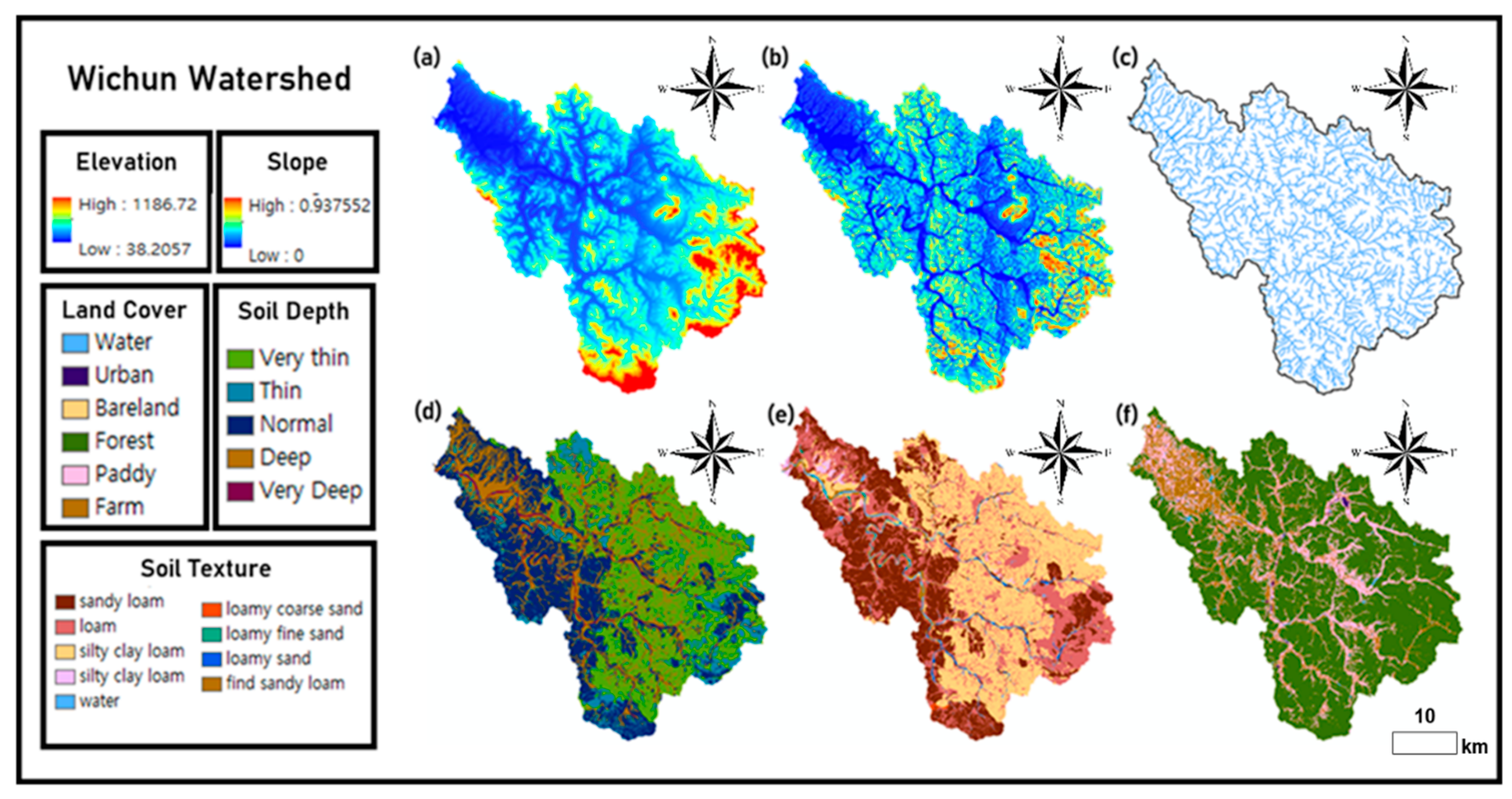
In the theoretical background of rainfall prediction and runoff analysis, numerous parameters for understanding nature are ruled by uncertainty. The deformation of artificial natural conditions is one of the numerous factors that increase uncertainty, including between the simulated and observed results. The target watershed of this study was selected as the Wicheon Basin in Korea [
4], which is located upstream of the hydrological cycle among the tributaries of the Nakdong River water system and can be considered because of its relatively low artificial hydrological control (
Figure 1).
2.2. Rainfall Events
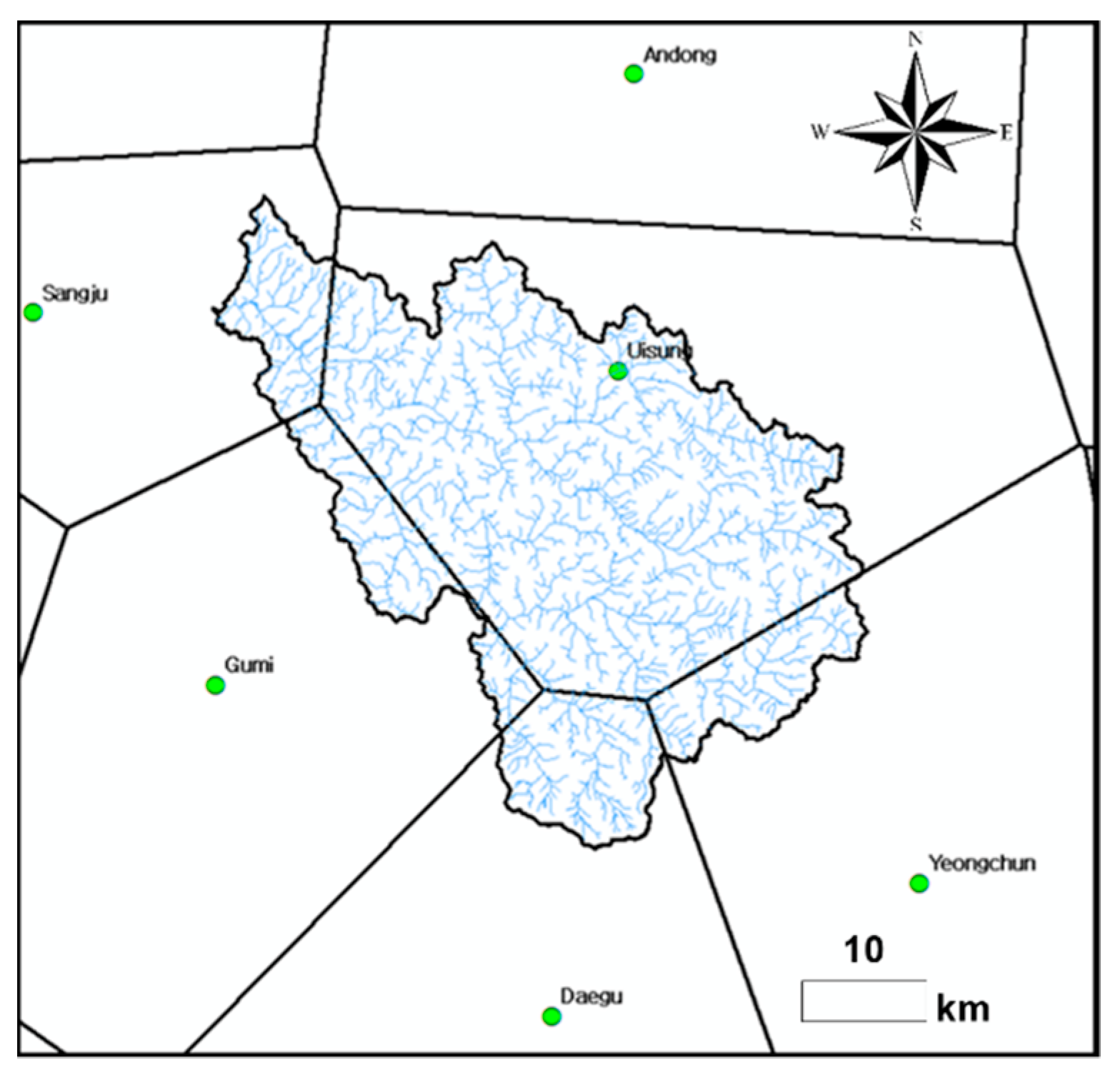
In this study, rainfall events were studied from June to October 2016 and May to September 2017 during the rainy season. In the Wicheon Basin, six LENS forecast data periods were selected, from 15/09/2016 00UTC to 17/09/2016 12UTC, using subsequent rainfall based on the rainfall events (Event W, E.W.) of up to 11 mm/h. Using the above six LENS predictions, the point and area values were calculated and schematized in the forecasting time–value graph. The applicability of LENS ensemble members according to the prediction time was evaluated using the three fit calculation methods. Branch rainfall was calculated by collecting hourly rainfall data from the Automated Surface Observation System (ASOS) provided by the Korea Meteorological Administration (KMA). Although there is an arithmetic mean method, Thiessen weighting method and isohyetal method for calculating area rainfall, the Thiessen weighting method was used in this study [
5]. The Thiessen weighting method calculates the average rainfall of the area by manufacturing the Thiessen network using the location of the observatory centered on the study target area and calculating the corresponding area ratio as a weight [
6]. The Thiessen network was created using the Create Thiessen tool of the ArcGIS program. The results of the Thiessen network in the Wicheon Basin are shown in
Figure 2. Thiessen weight was evaluated by calculating the ratio of the area of Thiessen corresponding to the rainfall observation station to the total area and the weight for each observation station, as shown in
Table 1.
2.3. Limited Area ENsemble Prediction System (LENS)
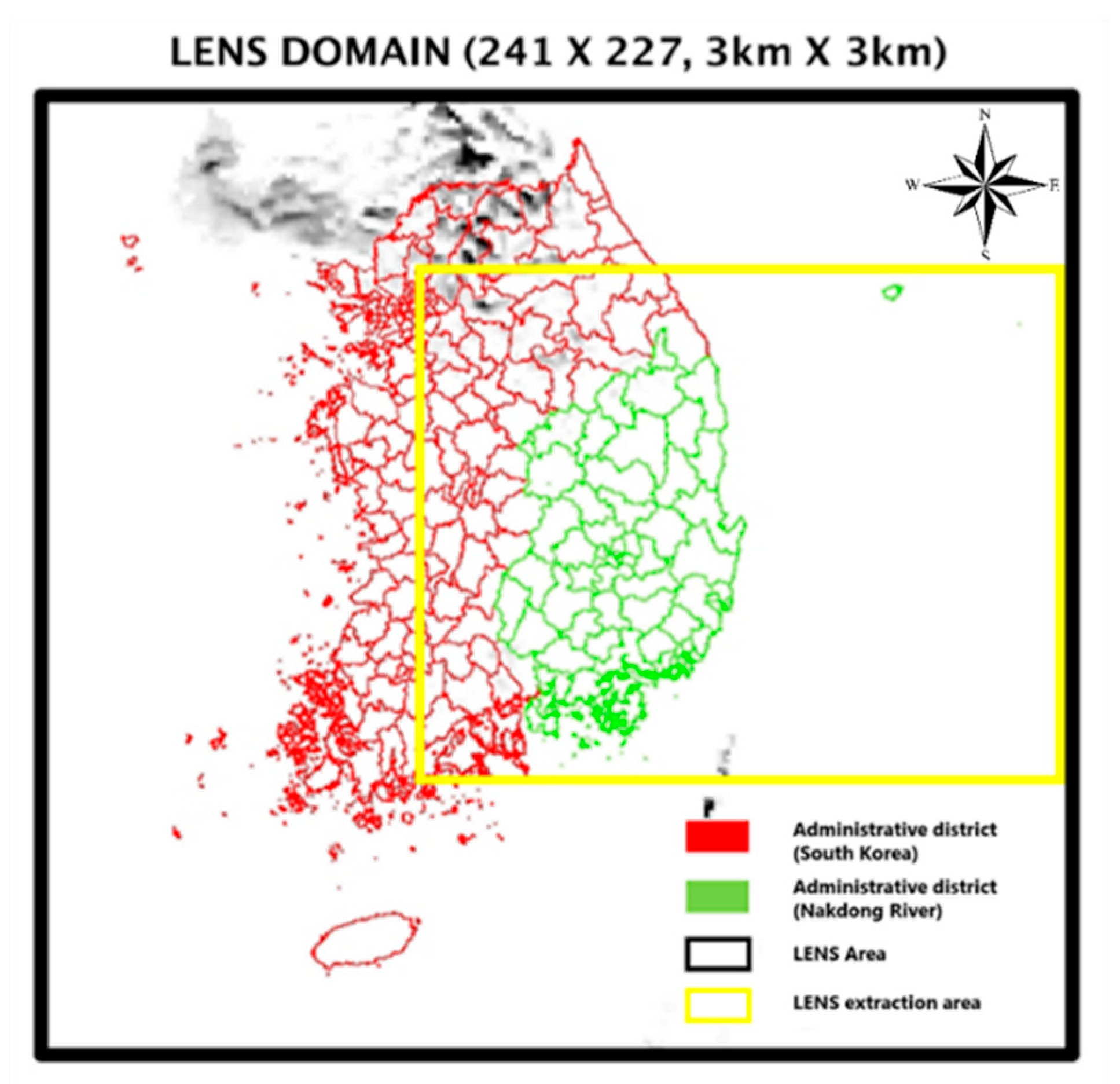
The Korea Meteorological Administration (KMA) has operated LENS since October 2015 to provide guidance for early warning by making probabilistic predictions of extreme weather. LENS has a horizontal resolution of 2.2 km and a prediction period of 72 h on 70 vertical floors and aims to predict the probability of dangerous weather on the Korean Peninsula. LENS was designed to predict the upcoming 72 h every 12 h based on the KMA global ensemble prediction system (EPSG). It consists of 13 members, one control member and 12 perturbation members, centered on the Korean Peninsula (
Figure 3).
LENS provides probability values for precipitation, snowfall, wind gust and predictions, such as temperature, total cloud volume, precipitation and wind speed [
2]. In this study, the total precipitation among the climate elements of LENS data was extracted. The precipitation observation value at the point of weather observation and the average precipitation value of the administrative district area were calculated based on the administrative district boundary. Then, the applicability of LENS was evaluated.
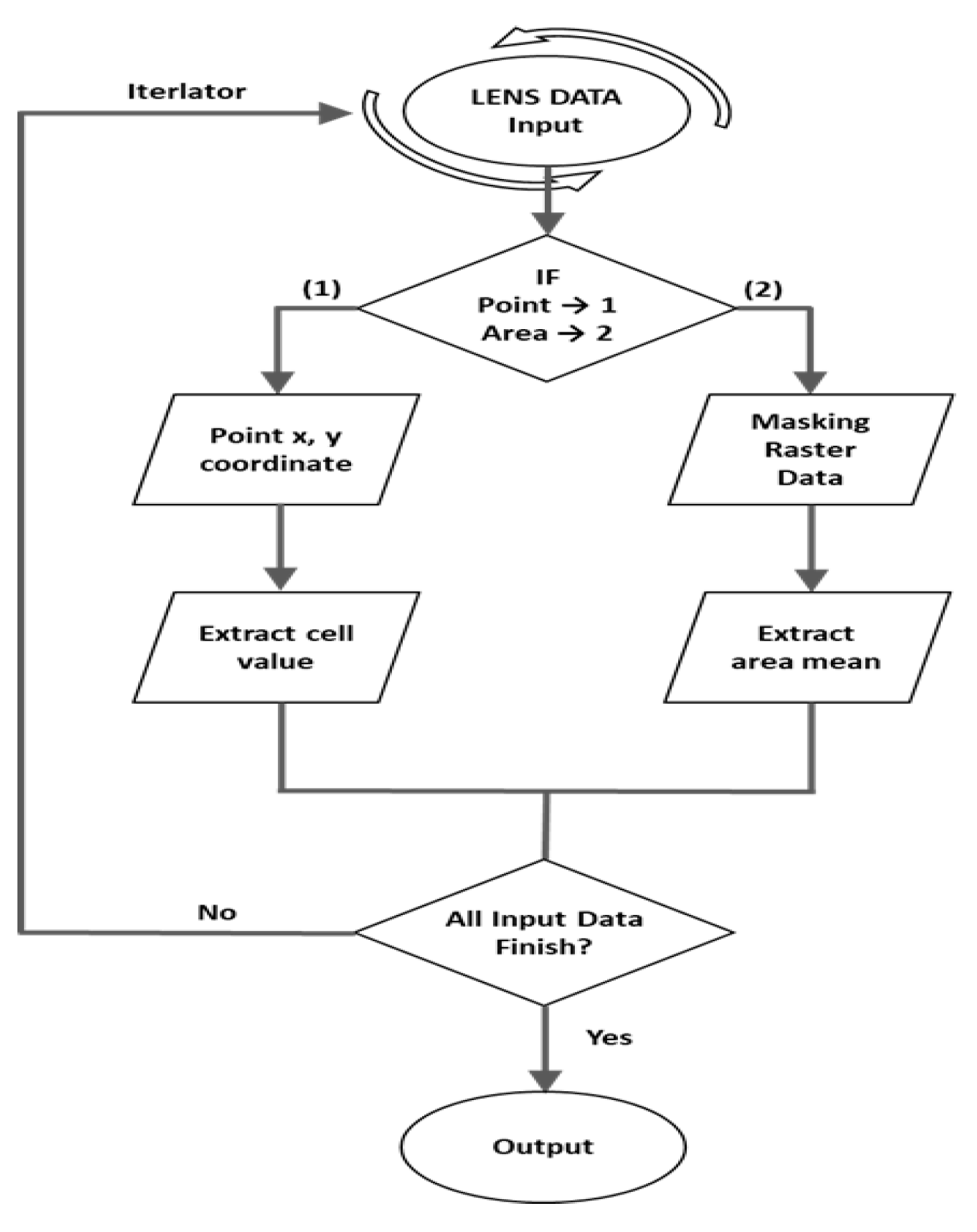
LENS data consist of one ASCII file per hour for a period of +04 h to +72 h for each of the 13 members of m00–m12 from the predicted start time. Spatial preprocessing is required for analysis according to the target basin and a long time is needed to process a large number of files and repetitive tasks manually. To this end, this study constructed LENS data for each target basin by utilizing the Arcpy module in the Python2 development environment provided by ArcGIS. Coding algorithms for each point and area are shown in
Figure 4.
2.4. Grid Based on Rainfall-Runoff Model (GRM)
The GRM simulates rainfall-runoff using a physical-based distributed model [
7]. In the GRM, runoff is largely divided into surface and direct runoff. Surface runoff uses overland flow and channel flow, whereas direct runoff uses surface runoff and subsurface flow. Surface runoff is caused by penetration overflow [
8] and saturation overflow [
9], and the penetration process and subsurface runoff are interpreted for the soil water zone [
10]. The overall hydrological component simulation process is illustrated in
Figure 5.
In this study, the flow rate data for verification of the GRM model were used in units of 10 min. The Yonggok water level station was selected, the discharge point was designated as the water level observation station point and the flow data were constructed. The discharge verification period was selected as the day on which the observed flow rate exceeded 800 m3/s in September 2016.
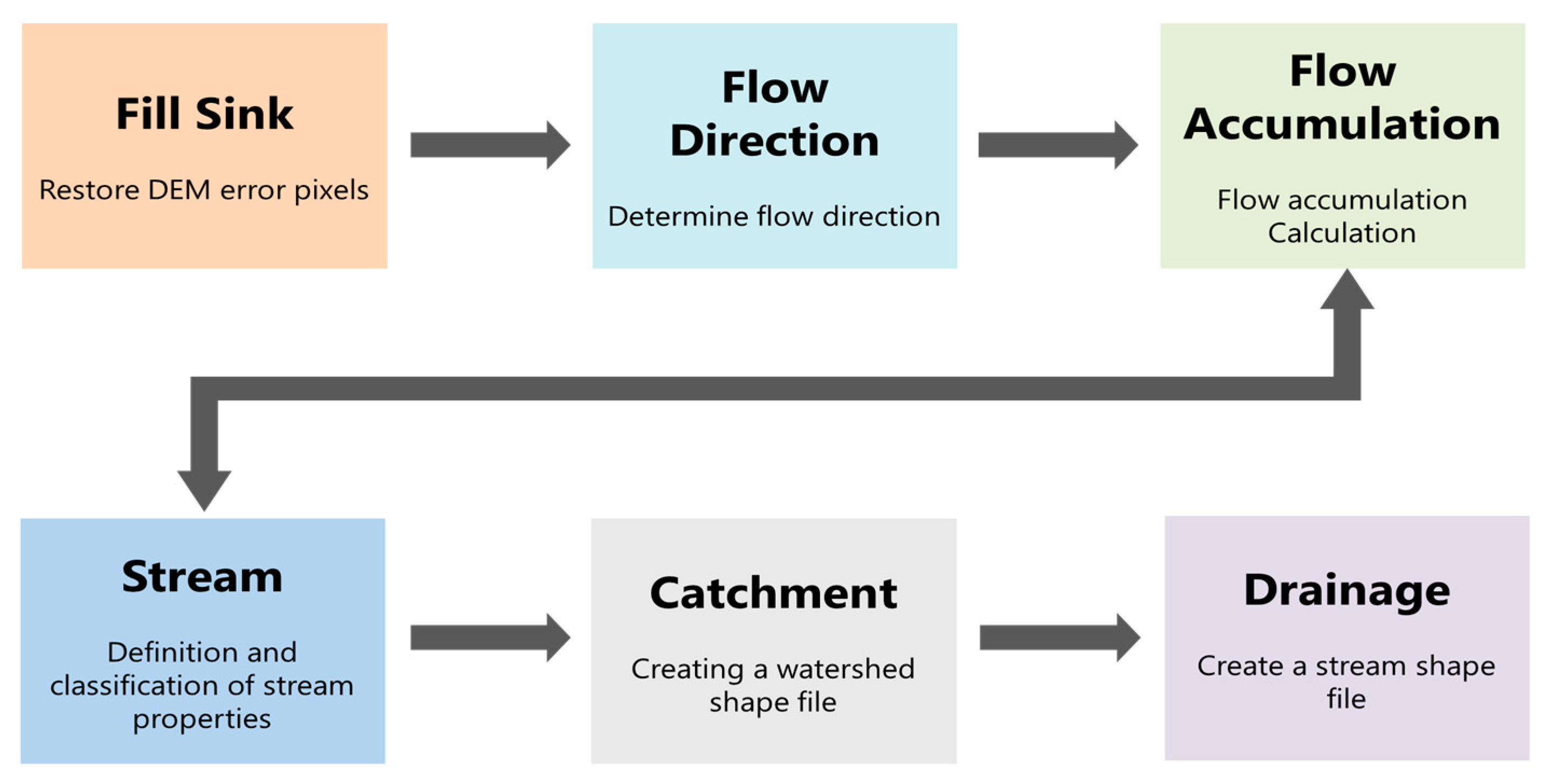
DEM was used to build the data necessary for the GRM model. Input data were constructed using a drainage tool for hydrological topographic factor analysis. A hydrological DEM was generated using a fill sink and the grid base flow direction was calculated using the flow direction. After calculating the cumulative number of flows through the flow direction grid previously generated by flow accumulation, river analysis was performed and the slope was calculated using the altitude for each grid of the DEM. The stream calculates the river grid based on the threshold value calculated by the flow accumulation and, in this study, the threshold value was set to 30 based on the DEM with a resolution of 90 m. Based on the schematic diagram of the drainage tool, topographic construction data for the target watersheds in the Wicheon Basin are shown in
Figure 5.
The applied parameters were IniSaturation, MinSlopeOF, ChRoughness, CalCoefLCRoughness, CalCoefSoilDepth, CalCoefPorosity, CalCoefWFSuctionHead and CalCoefHydraulicK and the range for each parameter was determined by setting the minimum and maximum ratios for each GRM parameter [
7]. The range and definition of each parameter are presented in
Table 2.
2.5. Likelihood for GLUE
Three verification methods were used to evaluate the accuracy of the rainfall prediction of LENS data and the applicability of the LENS-GRM model. To analyze the uncertainty of the GRM’s parameters, uncertainty analysis was performed using three likelihoods, informal likelihood NSE, PBIAS and formal likelihood log-normal. This is based on the GRM model parameter correction results using the General likelihood uncertainty estimation (GLUE), which interprets uncertainty based on the Bayesian theory of inducing the posterior distribution of parameters using likelihood functions and pre-distribution of parameters [
11]. In this study, R
2 = L
1, NSE = L
2, PBIAS = L
3 and log-normal = L
4 were used for readability.
The coefficient of determination R
2 was calculated as the square of the Pearson correlation coefficient r, representing the ratio of the total variance of the observed values to the simulated values. R
2 has a value from 0.0 to 1.0 and the closer
R2 = 1, the better the relationship [
12].
R2 is calculated as shown in Equation (1), where N represents the number of data points,
Ot and
Pt represent the actual rainfall and LENS rainfall at time
t and the average value of the actual rainfall and LENS rainfall.
Nash-Sutcliffe Efficiency (NSE) is a normalized statistic that determines the relative magnitude of the residual variance by comparing the variance of the data [
13]. It indicates how well the simulated and observed values fit the 1:1 line. NSE has a range of −∞ to 1.0 and the closer it is to 1, the closer the relationship. The NSE equation is shown in Equation (2), where N represents the number of data,
Ot and
Pt represent the actual rainfall and LENS rainfall at time
t, respectively, and is the average value of the actual rainfall.
Percent bias (PBIAS) is an evaluation index that represents the average trend of simulation data in percentage terms [
14]. PBIAS is a suitable index for distinguishing between underestimation and overestimation of the observed data. PBIAS = 0 represents an ideal optimal value, PBIAS < 0 represents an overestimation and PBIAS > 0 represents an underestimation. The equation of PBIAS is shown in Equation (3), where N represents the number of data and
Ytobs and
Ytsim represent the actual rainfall and LENS rainfall at time t.
Log-normal (log-likelihood function) is a log of likelihood functions using natural logarithms for the computational convenience of maximum likelihood estimation and measuring the fit between model parameters and observational data [
15]. When there is no criterion for a threshold, i.e., log-normal, the behavior model can be determined by selecting a portion of the upper value. In this study, the value of the upper 30% was considered as the behavior model [
16]. The log-normal distribution is shown in Equation (4).
Here, N is the number of observed values,
σ2 is the variance of the simulated value, which is equal to Equation (5),
εj(
θ) is the vector value of the residual, the difference between the simulated value and the observed value over time t, and is equal to Equation (6).
2.6. Behavioral Model Selection and Uncertainty Assessment
In this study, 2000 GRM parameters correction were performed first and second, respectively. During the initial correction, the number of behavioral models decreased owing to the wide range of parameters and the range of uncertainty increased. Therefore, after calculating the uncertainty range with the primary correction, the new parameter range was performed as a secondary correction to obtain the parameters optimized for the basin. The resulting value of the GRM model, according to parameter correction, was divided into a behavioral model and an non-behavioral model using the likelihood function of L
2, L
3 and L
4. Behavioral models were selected in the range L
2 > 0.65 [
17] L
3 < |25| [
18] and the top 30% L
4 [
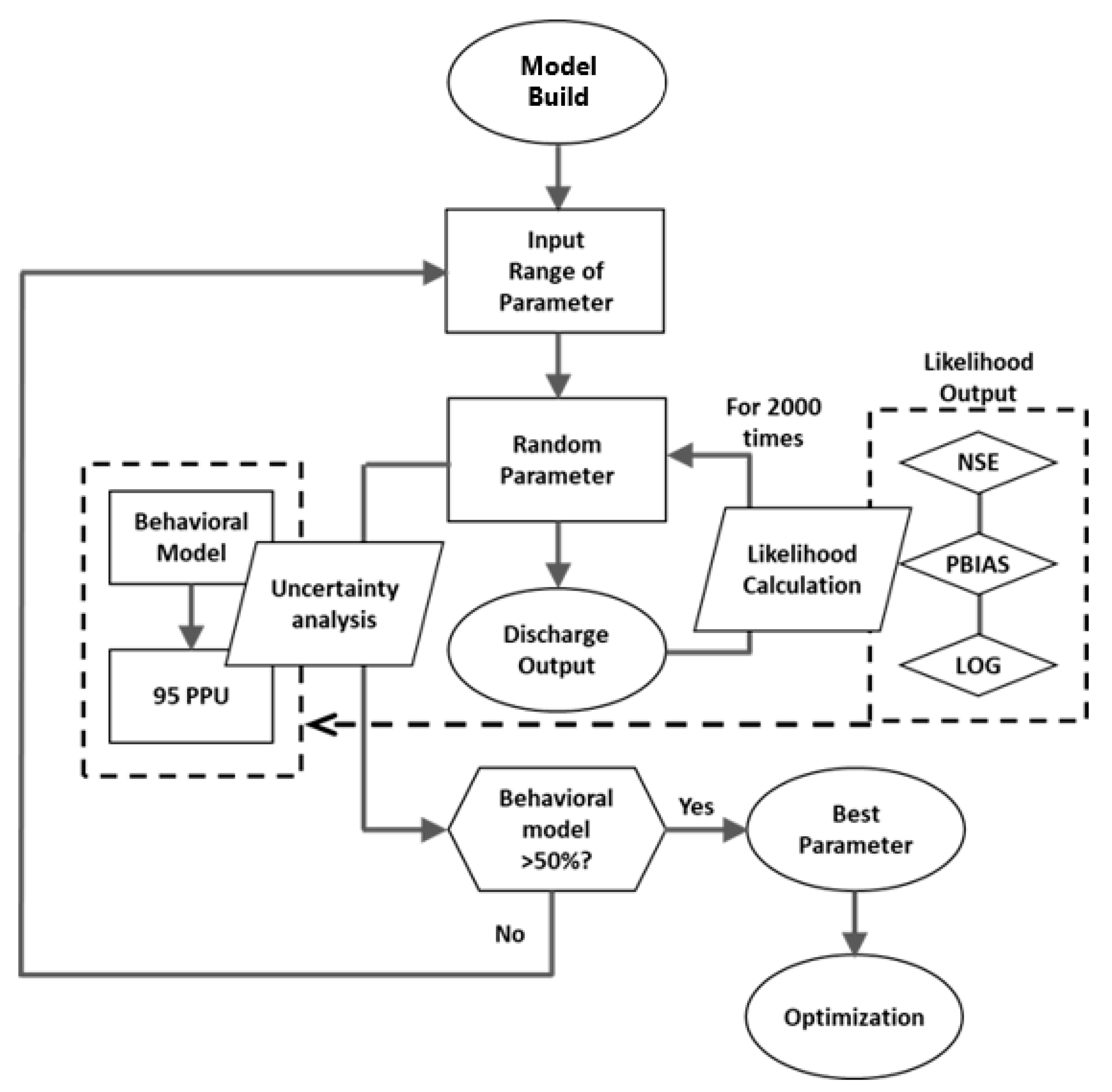
19] by likelihood. To calculate the optimal parameter value, a sensitivity analysis was conducted using the random parameter value and the likelihood function and the parameter sensitivity analysis was conducted using the cumulative histogram with the parameter value selected as the behavior model. In addition, the reliability and confidence interval of the behavior model were calculated using a 95% prediction uncertainty (95PPU) analysis and the best simulation results for each likelihood are shown. The process used for uncertainty evaluation is illustrated in
Figure 6.
3. Results
3.1. LENS Point and Area Applicability Analysis
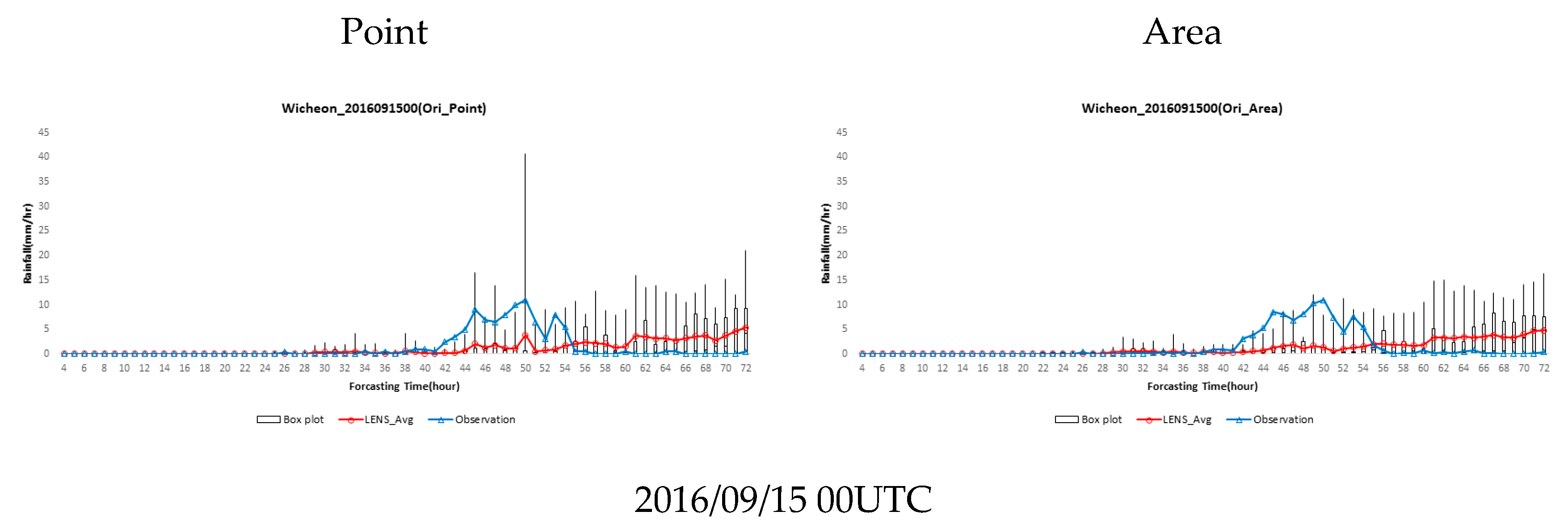
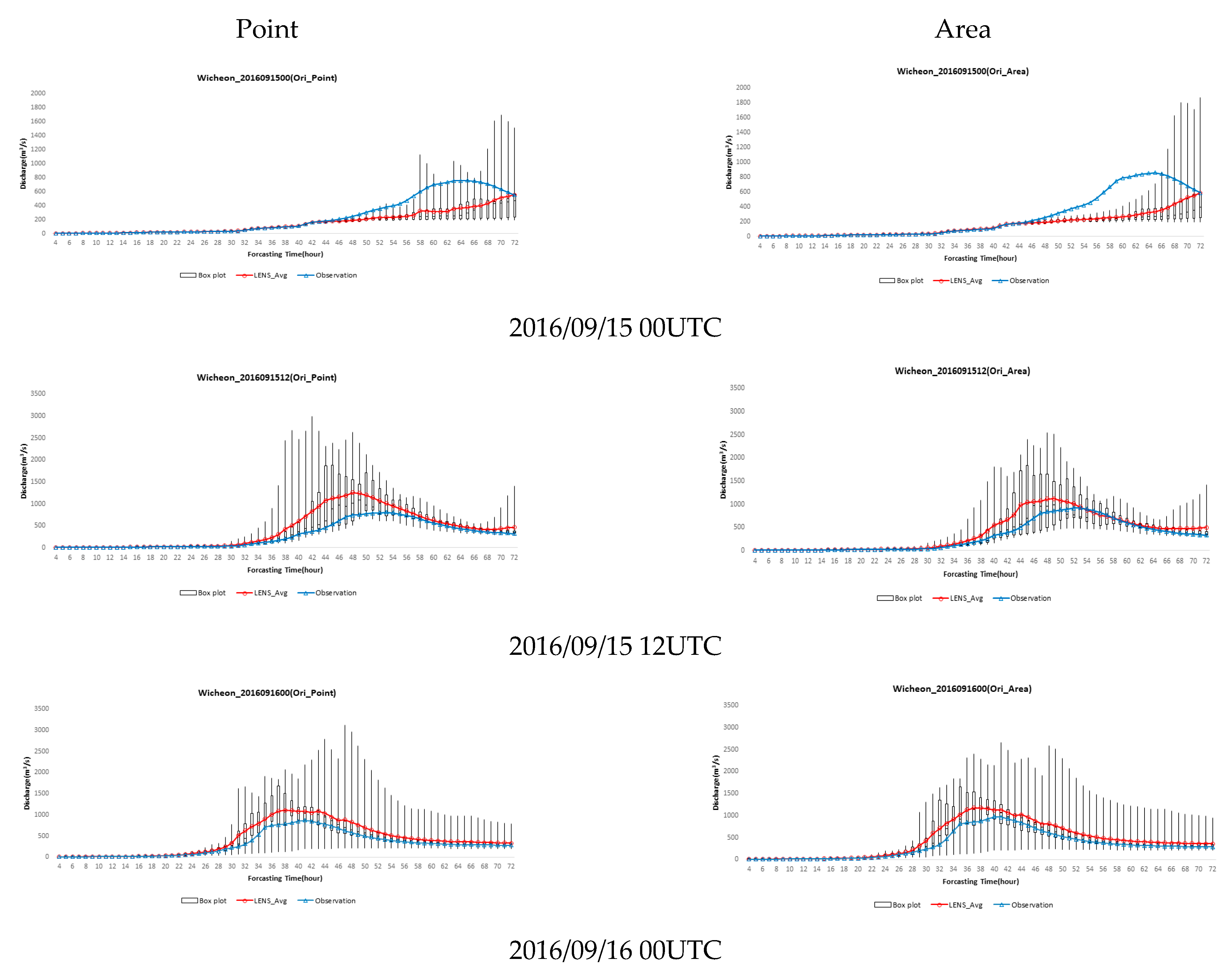
Figure 7 illustrates the point value and area average values for the LENS prediction value for the Wicheon basin. A red line denotes the LENS average value and a total of 13 LENS ensemble members were shaped as box plots. The observed value is shown by the blue line in
Figure 7. The average values of observation and LENS for each event were determined and are shown in
Table 3 as R
2(L1), NSE(L2) and PBIAS(L3).
Table 4 and
Table 5 present numerical information on LENS point value prediction results and observation values for each event. The numerical results of LENS area value prediction results and observation values for each event are included in
Table 6 and
Table 7.
2016/09/15/00UTC E.W. showed a tendency to predict delays more than peak time in both branch and area prediction data and to predict excessively from 55 h. The maximum tendency of the ensemble members showed that the area value was similar to the observation value and the point value was more than twice the prediction at 50 h. In the goodness-of-fit evaluation, L1, L2 and L3 showed higher point values.
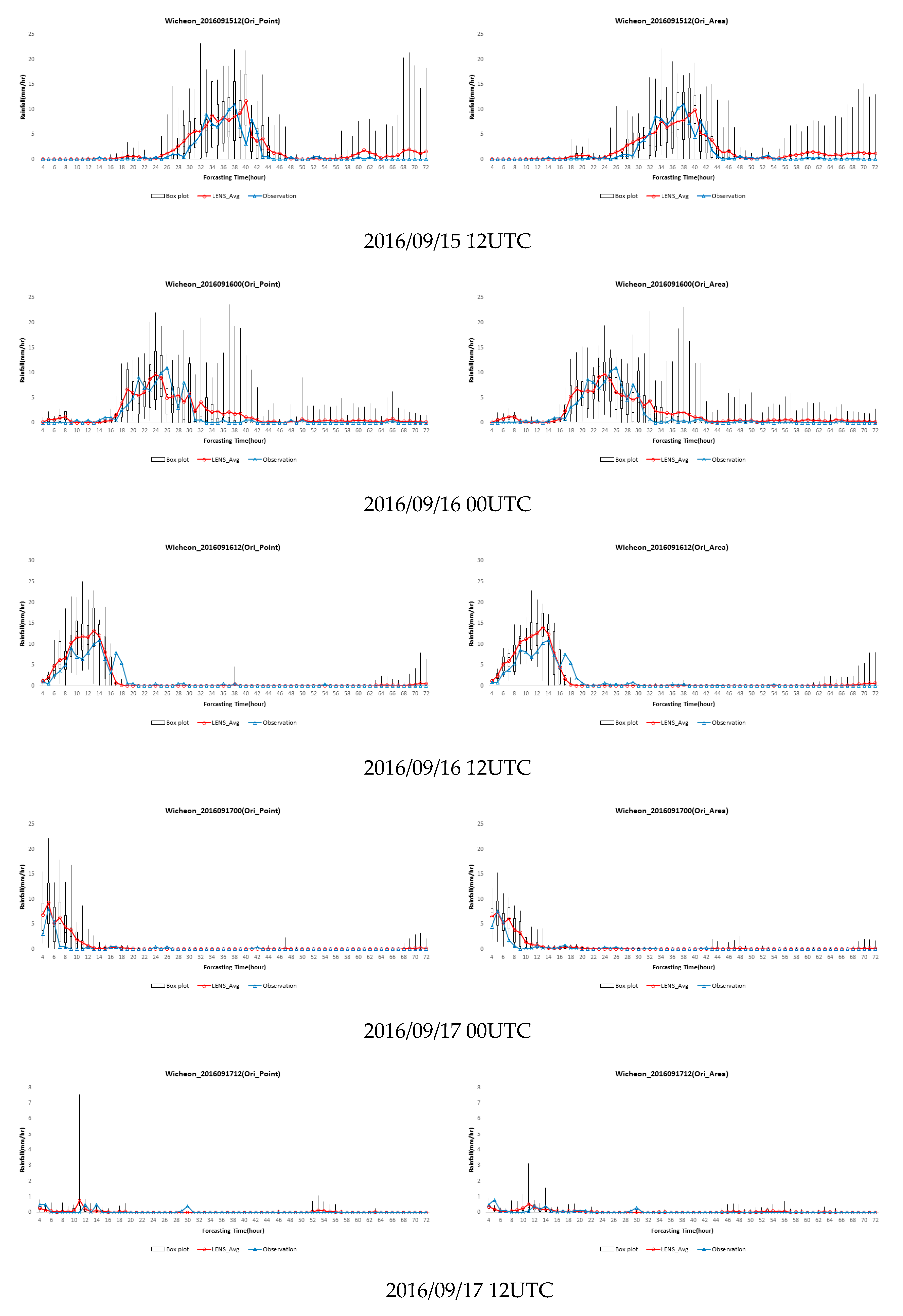
2016/09/15/12UTC E.W. showed a tendency very similar to the actual observation value for both point and area ensemble prediction average values. The box plot confirmed that the deviation of each ensemble member was large; however, it can be assumed that the actual observation value is included in the quartile range. In terms of fit, the area value was the highest for L1, L2 and L3. The total rainfall difference, peak rainfall difference and peak time difference showed slight differences and a high degree of accuracy.
2016/09/16/00UTC E.W. showed a similar trend to the 2016/09/15 12 UTC E.W. prediction data, showing a higher accuracy through suitability evaluation. L1, L2 and L3 showed higher area values and the difference in rainfall prediction was insignificant, indicating a high accuracy.
2016/09/16/12UTC E.W. showed the highest accuracy among the Event W predictions. It may be confirmed that the area value is higher at L1, L2 and L3 and the difference in rainfall prediction is highly accurate at both points and areas. In the box plot, the quartile range tended to slightly overestimate the observed values.
2016/09/17/00UTC E.W. is a prediction of 8 mm/h 4 h after Event W occurrence, the maximum range of the point value tends to be about 2.5 times over-predicted and the maximum range of the area value tends to be 1.5 times over-predicted. However, the tendency of the quartile range and average value showed a good tendency for the observed value. L1, L2 and L3 showed a higher area value and, in the difference in rainfall prediction, the area value was highly accurate with respect to the difference between time and peak value.
12/09/17/12UTC E.W. predicts data for rainfall of less than 1 mm/h after Event W, tending to overestimate the prediction of 11 h at points and areas. and shows low values in the L1, L2 and L3 suitability calculation results.
3.2. Event.W Parameter Post-Distribution by Likelihood
For the selection of an L
2-based behavioral model, L
2 > 0.65 was used as a threshold through calculation of parameters for each GRM likelihood. The number of L
2-based behavioral models was 1121 (56.05%). Among the L
2-based behavioral models, the sub-light coefficient and initial saturation parameters were the most sensitive. The ranges of the L
2-based behavioral models for each parameter are presented in
Table 8. In addition, to confirm the distribution of the L
2-based behavioral models by parameter, it is expressed as shown in
Figure 8, using the cumulative distribution function (CDF) and histogram.
For L
3-based behavioral model selection, |L
3| < 25 was used as a threshold by calculating the parameters for each GRM likelihood. The number of L
3-based behavioral models was 1151 (57.55%). Among the L
3-based behavioral models, the most sensitive parameter was the initial saturation. The ranges of the L
3-based behavioral models for each parameter are presented in
Table 9. In addition, to confirm the distribution of the L
3-based behavioral models by parameter, it is expressed as shown in
Figure 8, using the cumulative distribution function (CDF) and histogram.
The L
4-based behavioral model was selected as the threshold for the top 30% by calculating the parameters for each GRM likelihood. The number of L
4-based behavioral models was 600 (30%) [
7]. The L
4-based behavioral model was sensitive to the initial saturation, river roughness coefficient and soil depth.
Table 10 shows the range of the behavioral model based on each parameter. In addition, to confirm the distribution of L
4-based behavioral models by parameter, it is expressed as shown in
Figure 8, using the cumulative distribution function (CDF) and a histogram.
The number of behavioral models for each likelihood of Event. W was L2 = 1121, L3 = 1151 and L4 = 600. Accordingly, the cumulative distribution function (CDF) over time was calculated for the simulation discharge simulation value (Simulation Discharge) of the behavior model and 95% reliability analysis was conducted through the cumulative probability distribution.
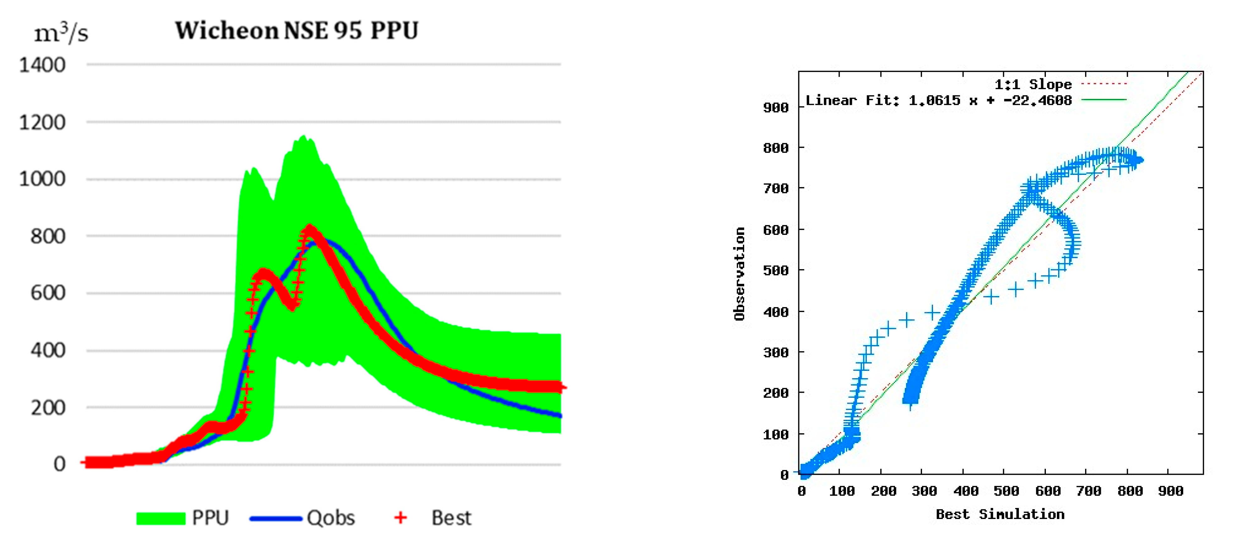
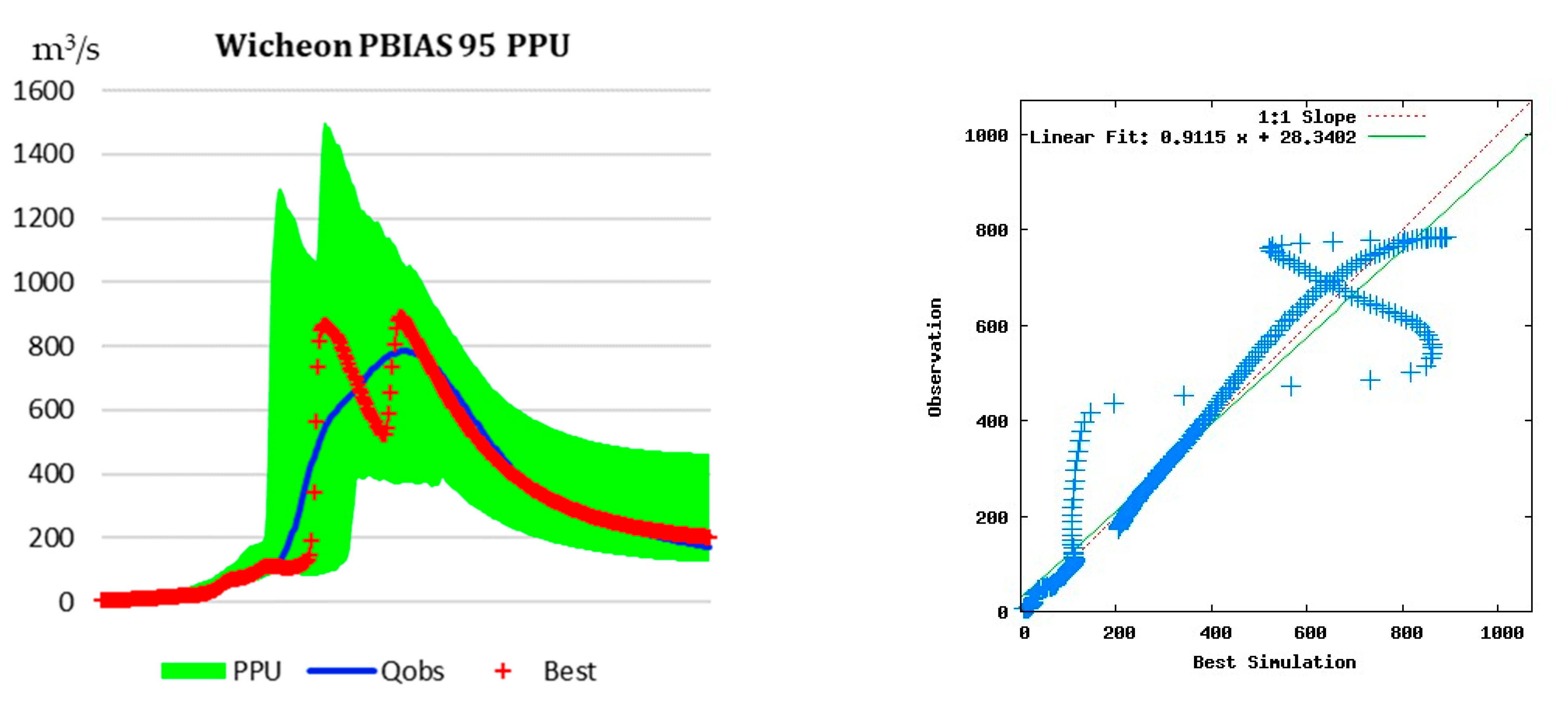
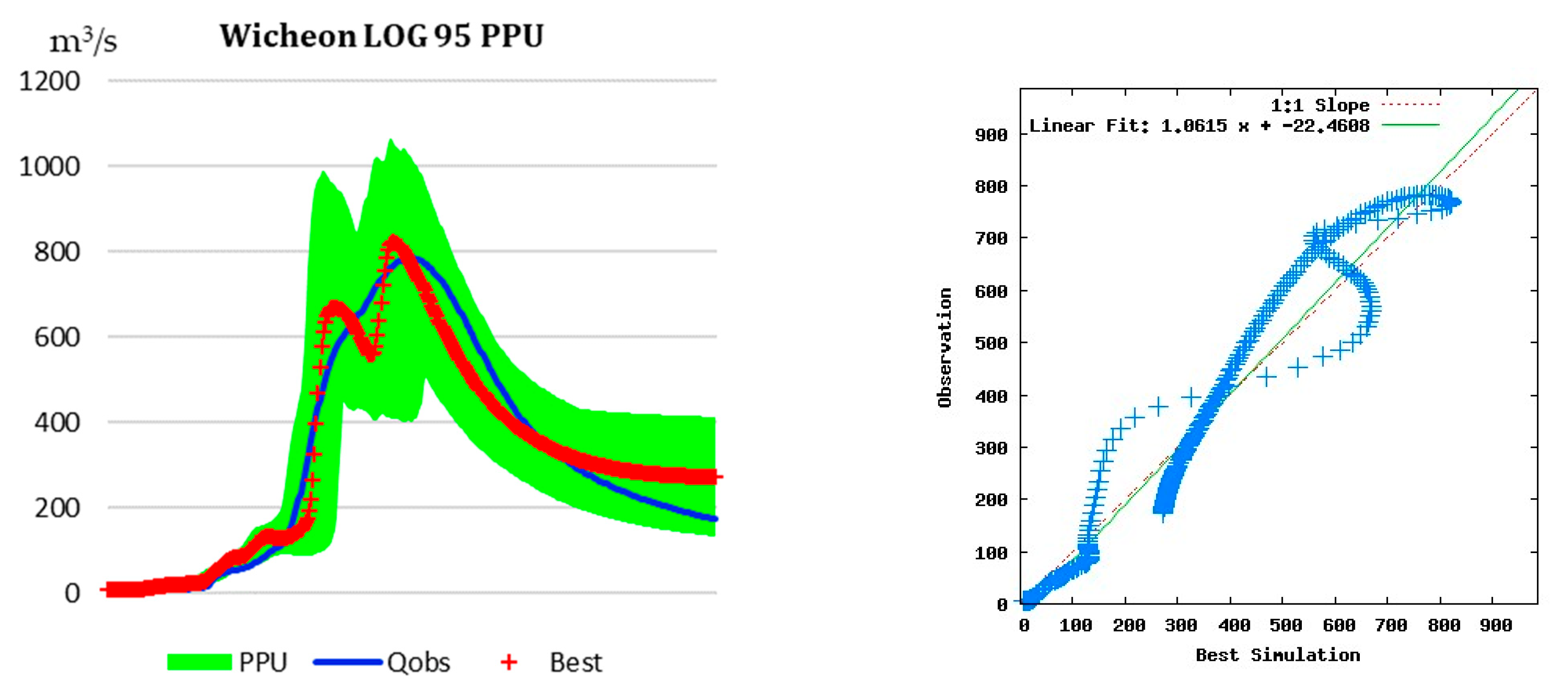
In
Figure 9,
Figure 10 and
Figure 11, the 95 PPU for the uncertainty of the L
2-based behavior model was shown as a green range, the L
2 95 PPU optimum value “best simulation” was shown as a red dotted line and the observed flow rate was shown as a solid blue line. The L
2-based behavioral model outflow simulation value was very similar to the observed flow rate. The L
2 value of Best Simulation was 0.9421, the highest value-based L
3 was |0.8081| and L
4 was −1924.25.
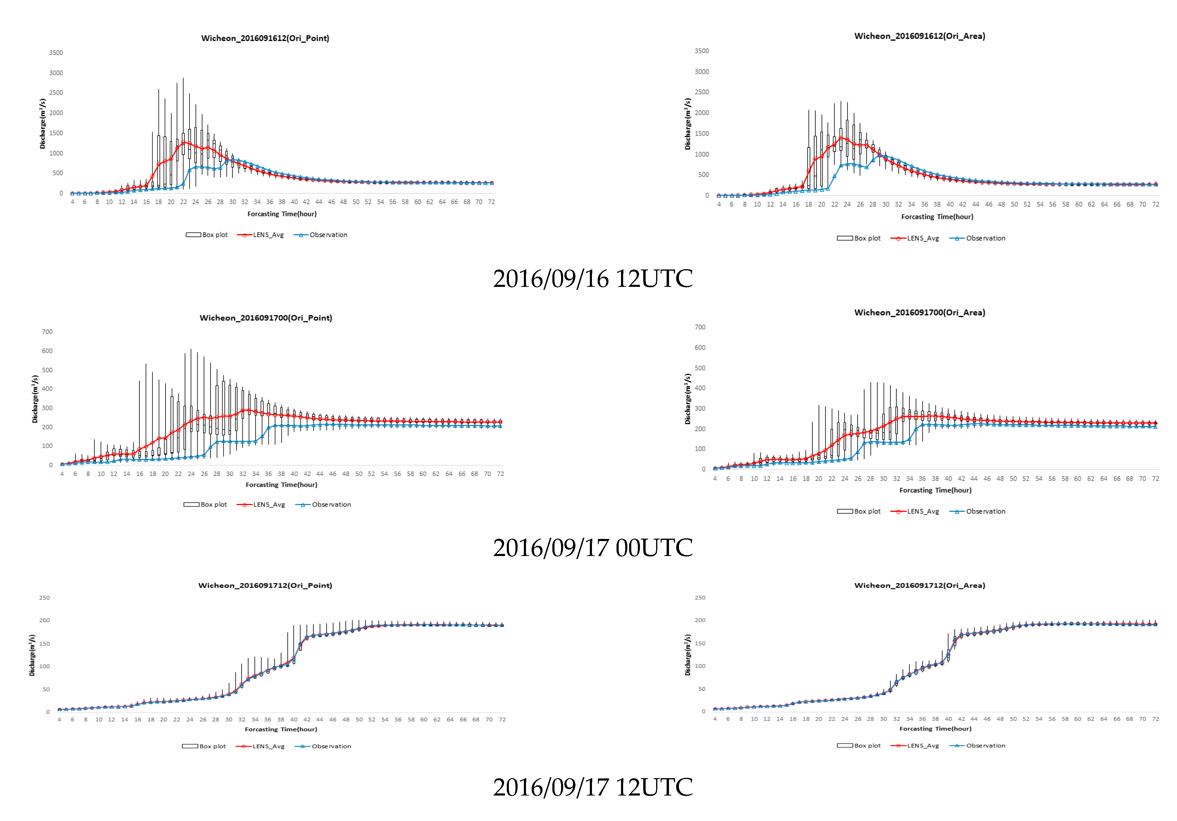
3.3. Application and Evaluation of the GRM Model
The prediction of LENS data in the Wicheon Basin was found to be highly accurate. Therefore, the outflow prediction simulation showed a tendency towards high suitability overall. The results of the LENS-GRM model simulation are expressed in a box plot over time in
Figure 12, and the likelihood is calculated for the observation value and the average value of the LENS ensemble members in
Table 11.
2016/09/15 00UTC GRM.W showed a high accuracy of leakage occurrence time. The point value tended to follow the tendency of the peak flow rate in the maximum value range and the area value tended to overestimate the maximum value range after the peak time. L1, L2 and L3 were higher at the point value, whereas L1 showed a higher fit of 0.8 L2 of 0.6.
In 2016/09/15 12UTC GRM.W, the average value of the outflow prediction mock was higher than the observed flow rate. In addition, the majority were distributed in a range higher than the median and have an overall tendency to overestimate. The area value had a smaller tendency to be overestimated than the point value. L1, L2 and L3 showed a higher fit with the area values.
In 2016/09/16 00UTC GRM.W, the deviation between the average value and the observed value of the outflow prediction mock, which showed an over-predictive tendency, was reduced. Unlike the previous data, which showed the trend of observation outflow in the minimum value range, it showed the trend of observation outflow in the first quartile range. L
1, L
2 and L
3 showed a very high suitability for both the points and areas in
Table 12 and
Table 13.
In the 2016/09/16 12UTC GRM.W, the outflow was predicted in an irregular pattern compared to the previous data that predicted the outflow with a gentle curve. The total outflow and peak outflow also tended to be overestimated compared to the previous data. The peak time also showed a tendency to be predicted early in the range of −6 to −8 at −3 h. By calculating suitability, L2 was also found to show a lower suitability compared to all data.
2016/09/17 00UTC GRM.W followed the trend of observation outflow in the minimum value range and showed a tendency to overestimate overall. The area value tended to be close to the first quartile range and showed a high value in suitability calculation results.
The 2016/09/17 12UTC GRM.W dataset showed a tendency to completely match the average value of the outflow prediction model and the observed outflow value. Accordingly, the result of calculating suitability was also found to be the highest optimum value and only some ensemble members showed excessive prediction in
Table 14 and
Table 15.
4. Discussion
The rainfall prediction accuracy of the LENS rainfall ensemble prediction data shows a higher accuracy as the prediction start time of the LENS data and the rainfall event occurrence time approach each other. In addition, the prediction uncertainty increased as the prediction start time and rainfall event occurrence time increased. In the ensemble, this is called spread or uncertainty, which is the standard deviation of each member for the average of the ensemble members. The longer the prediction time, the wider the range of predictions. This is one of the representative uncertainties in rainfall ensemble predictions. Regardless of how small the error in the initial rainfall ensemble prediction, the magnitude of the error may increase exponentially as the nonlinear model integrates with the initial perturbation member [
20]. Thus, prediction accuracy can be enhanced by filtering uncertain prediction information with ensemble averages for multiple initial perturbation members for the initial conditions [
21].
The spatial characteristics of the LENS rainfall ensemble prediction data were calculated and compared with the rainfall observation station point and basin area values for the study target basin. The results of the applicability analysis through the fitness index confirmed that the value could not be said to be better and the difference was also insignificant. This may have an effect on the uncertainty that occurs when the spatial distribution of the study target is small compared to the 3 km resolution among the characteristics of the LENS data. In addition, the criteria for calculating the suitability of the rainfall ensemble members were analyzed by comparing them with the ground rainfall observation values. At this time, the accuracy of rainfall prediction caused by the uncertainty in ground rainfall observations cannot be excluded [
22]. Accordingly, the applicability analysis of LENS data may be improved by subsequent studies, i.e., (1) uncertainty analysis of perturbation members using ensemble averages; (2) expansion of target areas; (3) uncertainty analysis between ground rainfall observation and ensemble prediction; (4) accuracy according to topographic location.
The final goal of this study was to evaluate the applicability of outflow prediction in the case of outflow simulation using the GRM model as input data for LENS prediction data. Accordingly, to calculate the simulated flow rate that is most similar to the observed flow rate for each target basin, optimization of the parameters for each basin was performed. With respect to the sensitivity of the GRM model parameters, the initial saturation and sub-luminance coefficients were the most sensitive. Hydrologically, the lower the initial saturation, the greater the infiltration of rainfall owing to the decrease in the soil moisture content and the decrease in the overall outflow. As the channel roughness coefficient increased with the degree of resistance (friction) of the channel to the flow, the time of the peak flow rate was delayed. It is believed that the topographic factor of the model verification area by basin plays the largest role. In this study, most of the target watersheds were in mountainous terrains and the verification area was located upstream. Compared to that in other regions, it is expected that the inflow rate of rainfall into the river is faster in the event of rainfall and that an immediate outflow will occur. It is also expected that immediate rainfall penetration will occur in impermeable areas (compared to that in many urbanized basins).
With respect to parameter correction, the uncertainty range of the fitness index for all target watersheds was found to be significantly improved. In addition, the sensitivity of the parameter changes to an even shape through the point distribution and histogram. Equal parameter sensitivity is not a good result as it cannot further narrow the scope of a specific behavioral model within that range. Analysis of uncertainty by likelihood through 95PPU revealed that the uncertainty range during the second correction narrowed and improved compared to the first correction. However, this is also associated with many uncertainties. There is still no definitive inference regarding the scope in setting the scope of the behavior model, which relies on empirical research standards. Therefore, the outflow value of the GRM best simulation by basin also showed a high degree of consistency with the observed flow rate and the flow rate occurrence time. In contrast, this should be verified by investigating more uncertainty research cases to obtain the optimal outflow characteristics for each time.
LENS rainfall ensemble prediction data were analyzed for each target basin as the rainfall input data for the GRM. The results indicate that the simulated outflow value of the GRM accurately reflects the rainfall characteristics, which is the input data. The longer the prediction time, the lower the prediction accuracy; the shorter the prediction time, the higher the accuracy. For example, the characteristics of the rain prediction applicability analysis of the LENS ensemble prediction data are reflected in the outflow simulation. In the suitability evaluation of the outflow simulation using suitability likelihood, more evaluations are close to the optimum value for each likelihood than the rainfall prediction suitability evaluation. The accuracy of the ensemble members differed based on the period of comparison between points and areas and the difference was insignificant. This is believed to work with other factors and will need to be investigated in future studies.
5. Conclusions
The calculation of future rainfall prediction and outflow prediction is based on numerous hydrological, topographic and physical theories, as well as on the characteristics of input data and natural conditions. Each parameter is associated with many uncertainties, including an incomplete understanding of natural phenomena and the simplification of assumptions for user convenience, thereby giving rise to a high degree of uncertainty.
In this study, after analyzing the applicability of LENS, we analyzed the uncertainty of the outflow of rainfall ensemble prediction data using a grid-based rainfall-runoff model (GRM) model. The target basin of the Wicheon Stream was selected and hydrological and topographic data were constructed based on this basin. In addition, an accuracy analysis of the point and area rainfall prediction for each member of the target watershed LENS rainfall ensemble prediction data was conducted. Based on the constructed input data, the parameters were analyzed based on the likelihood, using the GRM model for each target basin. Finally, after calculating the optimal parameters for each target basin, the outflow simulation was analyzed using LENS rainfall ensemble prediction data as input data for the GRM model.
In the LENS data rainfall prediction applicability analysis, the closer the prediction start time and rainfall event occurrence time of LENS data, the higher the accuracy. As for the difference between the point value and the area value, the accuracy of the ensemble members differed according to the period.
In the GRM parameter correction study, the target watersheds exhibited the most sensitive appearance with respect to the initial saturation and underwater roughness coefficients. The tendency of the observed outflow value and simulated outflow value was optimized by calculating the optimal parameters for each target basin using parameter correction.
In the LENS-GRM outflow simulation, the simulated outflow value of the GRM appropriately reflected the characteristics of the rainfall input data. Similar to the characteristics of the LENS rainfall prediction analysis, the accuracy of the outflow simulation increased according to the accuracy of the input data.
Therefore, in this study, it was possible to confirm the temporal uncertainty of rainfall prediction using LENS data, the changes that bring about rainfall prediction and outflow prediction and the uncertainty of behavior model selection using the threshold of likelihood when applying the outflow model of rainfall prediction data. This is expected to reduce the uncertainty of the rainfall ensemble data and the uncertainty of applying the outflow model in selecting the behavior model of the user’s uncertainty interpretation. In addition, the application of research methods, i.e., characteristics of rainfall ideology and geographical characteristics, as well as the expansion of analysis targets, can be used as the basis for future rainfall and flood prediction research.
Author Contributions
Conceptualization, S.L., Y.J. and Y.S.; Methodology, S.L.; Software, S.L. and Y.S.; Validation, S.L.; Formal Analysis, S.L.; Investigation, S.L., Y.S. and Y.J.; Resources, S.L., Y.J. and Y.S.; Data Curation, S.L., Y.S. and Y.S.; Writing—Original Draft Preparation, S.L., Y.J. and Y.S.; Writing—Review & Editing, S.L., Y.S. and Y.J.; Visualization, S.L.; Supervision, Y.J.; Project Administration, Y.J.; Funding Acquisition, Y.J. All authors have read and agreed to the published version of the manuscript.
Funding
This research was supported by a grant (2022-MOIS61-001) of Development Risk Prediction Technology of Storm and Flood For Climate Change based on Artificial Intelligence funded by Ministry of Interior and Safety (MOIS, Republic of Korea).
Acknowledgments
Jung, Y. acknowledged the financial support of the Department of Advanced Science and Technology Convergence at Kyungpook National University. The authors acknowledge the efforts of the anonymous reviewers that worked on the manuscript.
Conflicts of Interest
The authors declare no conflict of interest.
References
- Bauer, P.; Auligné, T.; Bell, W.; Geer, A.; Guidard, V.; Heilliette, S.; Kazumori, M.; Kim, M.-J.; Liu, E.H.-C.; McNally, A.P.; et al. Satellite cloud and precipitation assimilation at operational NWP centres. Q. J. R. Meteorol. Soc. 2011, 137, 1934–1951. [Google Scholar] [CrossRef]
- Korea Meteorological Administration Republic of Korea (KMA). Joint WMO Technical Progress Report on the Global Data Processing and Forecasting System and Numerical Weather Prediction Research Activities for 2016; Korea Meteorological Administration Republic of Korea (KMA): Seoul, Republic of Korea, 2016.
- Lee, M.; Kang, N.; Kim, J.; Kim, H.S. Estimation of optimal runoff hydrograph using radar rainfall ensemble and blending technique of rainfall-runoff models. J. Korea Water Resour Assoc. 2018, 51, 221–233. [Google Scholar]
- Ministry of Construction and Transportation Gyeongsangbuk-do. The Basic Plan for River Maintenance in Wicheon; Ministry of Construction and Transportation: Sejong, Republic of Korea, 1998. [Google Scholar]
- Lee, S.-M.; Kang, H.-S.; Kim, Y.-H.; Byun, Y.-H.; Cho, C. Verification and Comparison of Forecast Skill between Global Seasonal Forecasting System Version 5 and Unified Model during 2014. Atmosphere 2016, 26, 59–72. [Google Scholar] [CrossRef]
- Lee, B.-J.; Bae, D.-H.; Jeong, C.-S. Runoff Curve Number Estimation for Cover and Treatment Classification of Satellite Image(II):—Application and Verification. J. Korea Water Resour. Assoc. 2003, 36, 999–1012. [Google Scholar] [CrossRef]
- Seong, Y.; Choi, C.-K.; Jung, Y. Assessment of Uncertainty in Grid-Based Rainfall-Runoff Model Based on Formal and Informal Likelihood Measures. Water 2022, 14, 2210. [Google Scholar] [CrossRef]
- Horton, R.E. The Rôle of infiltration in the hydrologic cycle. Trans. Am. Geophys. Union 1933, 14, 446–460. [Google Scholar] [CrossRef]
- Dunne, T.; Black, R.D. An Experimental Investigation of Runoff Production in Permeable Soils. Water Resour. Res. 1970, 6, 478–490. [Google Scholar] [CrossRef]
- Bras, R.L. Hydrology: An Introduction to Hydrologic Science; Addison Wesley Publishing Company: Boston, MA, USA, 1990. [Google Scholar]
- Jin, X.; Xu, C.-Y.; Zhang, Q.; Singh, V. Parameter and modeling uncertainty simulated by GLUE and a formal Bayesian method for a conceptual hydrological model. J. Hydrol. 2010, 383, 147–155. [Google Scholar] [CrossRef]
- Krause, P.; Boyle, D.P.; Bäse, F. Comparison of different efficiency criteria for hydrological model assessment. Adv. Geosci. 2005, 5, 89–97. [Google Scholar] [CrossRef]
- Nash, J.E.; Sutcliffe, J.V. River flow forecasting through conceptual models part I—A discussion of principles. J. Hydrol. 1970, 10, 282–290. [Google Scholar] [CrossRef]
- Legates, D.R.; McCabe Jr, G.J. Evaluating the use of “goodness-of-fit” measures in hydrologic and hydroclimatic model validation. Water Resour. Res. 1999, 35, 233–241. [Google Scholar] [CrossRef]
- Nourali, M.; Ghahraman, B.; Pourreza-Bilondi, M.; Davary, K. Effect of formal and informal likelihood functions on uncertainty assessment in a single event rainfall-runoff model. J. Hydrol. 2016, 540, 549–564. [Google Scholar] [CrossRef]
- Beven, K.; Binley, A. The future of distributed models: Model calibration and uncertainty prediction. Hydrol. Process. 1992, 6, 279–298. [Google Scholar] [CrossRef]
- Moriasi, D.N.; Gitau, M.W.; Pai, N.; Daggupati, P. Hydrologic and water quality models: Performance measures and evaluation criteria. Trans. ASABE 2015, 58, 1763–1785. [Google Scholar]
- Beven, K.J.; Kirkby, M.J. A physically based, variable contributing area model of basin hydrology/Un modèle à base physique de zone d’appel variable de l’hydrologie du bassin versant. Hydrol. Sci. J. 1979, 24, 43–69. [Google Scholar] [CrossRef]
- Ajmal, M.; Kim, T.W. Quantifying excess stormwater using SCS-CN–based rainfall runoff models and different curve number determination methods. J. Irrig. Drain. Eng. 2015, 141, 04014058. [Google Scholar] [CrossRef]
- Lorenz, E. The butterfly effect. World Sci. Ser. Nonlinear Sci. Ser. A 2000, 39, 91–94. [Google Scholar]
- Leutbecher, M.; Palmer, T.N. Ensemble forecasting. J. Comput. Phys. 2008, 227, 3515–3539. [Google Scholar] [CrossRef]
- Kang, N.; Joo, H.; Lee, M.; Kim, H.S. Generation of radar rainfall ensemble using probabilistic approach. J. Korea Water Resour. Assoc. 2017, 50, 155–167. [Google Scholar]
Figure 1.
Main features of Wicheon watershed. (a) DEM; (b) Slope; (c) Stream; (d) Land cover; (e) Soil depth; (f) Soil texture.
Figure 1.
Main features of Wicheon watershed. (a) DEM; (b) Slope; (c) Stream; (d) Land cover; (e) Soil depth; (f) Soil texture.
Figure 2.
Wicheon Thiessen Polygon.
Figure 2.
Wicheon Thiessen Polygon.
Figure 4.
LENS analysis algorithm.
Figure 4.
LENS analysis algorithm.
Figure 6.
GRM uncertainty analysis algorithm.
Figure 6.
GRM uncertainty analysis algorithm.
Figure 7.
LENS-observation forecasting time-value graph (Wicheon, event W).
Figure 7.
LENS-observation forecasting time-value graph (Wicheon, event W).
Figure 8.
Distribution of L3−based behavioral models by parameter (a1–a8) NSE results; (b1–b8) PBIAS results; (c1–c8) LOG results.
Figure 8.
Distribution of L3−based behavioral models by parameter (a1–a8) NSE results; (b1–b8) PBIAS results; (c1–c8) LOG results.
Figure 9.
NSE 95 PPU for uncertainty of L2-based behavior model.
Figure 9.
NSE 95 PPU for uncertainty of L2-based behavior model.
Figure 10.
PBIAS 95 PPU for uncertainty of L2-based behavior model.
Figure 10.
PBIAS 95 PPU for uncertainty of L2-based behavior model.
Figure 11.
LOG 95 PPU for uncertainty of L2-based behavior model.
Figure 11.
LOG 95 PPU for uncertainty of L2-based behavior model.
Figure 12.
Wicheon Original GRM Discharge (GRM. WOri).
Figure 12.
Wicheon Original GRM Discharge (GRM. WOri).
Table 1.
Theissen weight for each rainfall station in Wicheon watershed.
Table 1.
Theissen weight for each rainfall station in Wicheon watershed.
| Wicheon |
|---|
| Rainfall Station Name | Station Weight (%) |
|---|
| Uiseong | 67.55% |
| Daegu | 9.31% |
| Gumi | 8.70% |
| Yeongcheon | 7.51% |
| Sangju | 6.93% |
Table 2.
Parameters of the GRM model.
Table 2.
Parameters of the GRM model.
| Num | Parameters | Description | Range |
|---|
| Lower | Upper |
|---|
| 1 | IniSaturation (ISSR) | Initial soil saturation ratio | 0 | 1 |
| 2 | MinSlopeOF (MSLS) | Minimum slope of land surface | 0.0001 | 0.01 |
| 3 | ChRoughness (CRC) | Channel roughness coefficient | 0.008 | 0.2 |
| 4 | CalCoefLCRoughness (CLCRC) | Channel roughness coefficient | 0.6 | 1.3 |
| 5 | CalCoefSoilDepth (CSD) | Correction factor for soil depth | 0.8 | 1.2 |
| 6 | CalCoefPorosity (CSP) | Correction factor for soil porosity | 0.9 | 1.1 |
| 7 | CalCoefWFSuctionHead (CSWS) | Correction factor for soil wetting front suction head | 0.25 | 4 |
| 8 | CalCoefHydraulicK (CSHC) | Correction factor for soil hydraulic conductivity | 0.05 | 20 |
Table 3.
Point and area estimates for LENS data.
Table 3.
Point and area estimates for LENS data.
| Date | Point | Area |
|---|
| L1 | L2 | L3 | L1 | L2 | L3 |
|---|
| 2016/09/15 00UTC | 0.020 | −0.125 | 18.17 | 0.006 | −0.171 | 24.34 |
| 2016/09/15 12UTC | 0.721 | 0.648 | −42.95 | 0.816 | 0.796 | −26.68 |
| 2016/09/16 00UTC | 0.736 | 0.716 | −28.03 | 0.807 | 0.789 | −25.06 |
| 2016/09/16 12UTC | 0.806 | 0.654 | −17.95 | 0.847 | 0.709 | −13.97 |
| 2016/09/17 00UTC | 0.640 | 0.117 | −111.25 | 0.743 | 0.548 | −60.77 |
| 2016/09/17 12UTC | 0.092 | −0.175 | −5.13 | 0.324 | 0.302 | −12.10 |
Table 4.
LENS point data from 2016/09/15 00UTC to 2016/09/16 00UTC.
Table 4.
LENS point data from 2016/09/15 00UTC to 2016/09/16 00UTC.
| Wicheon (Point) | 2016/09/15 00UTC | 2016/09/15 12UTC | 2016/09/16 00UTC |
|---|
| Obs | LENS | Obs | LENS | Obs | LENS |
|---|
| Total rainfall | 93 | 76.11 | 93.5 | 133.66 | 93.6 | 119.84 |
| Total rainfall error | −16.89 | 40.16 | 26.24 |
| Peak rainfall | 11 | 5.41 | 11 | 11.65 | 11 | 9.71 |
| Peak rainfall error | −5.59 | 0.65 | −1.29 |
| Peak time | 50 | 72 | 38 | 40 | 26 | 24 |
| Peak time error | 22 | 2 | −2 |
Table 5.
LENS point data from 2016/09/16 12UTC to 2016/09/17 12UTC.
Table 5.
LENS point data from 2016/09/16 12UTC to 2016/09/17 12UTC.
| Wicheon (Point) | 2016/09/16 12UTC | 2016/09/17 00UTC | 2016/09/17 12UTC |
|---|
| Obs | LENS | Obs | LENS | Obs | LENS |
|---|
| Total rainfall | 91 | 107.33 | 20.5 | 43.31 | 2.5 | 2.63 |
| Total rainfall error | 16.33 | 22.81 | 0.13 |
| Peak rainfall | 11 | 13.24 | 8 | 9.29 | 0.5 | 0.77 |
| Peak rainfall error | 2.24 | 1.29 | 0.27 |
| Peak time | 14 | 13 | 5 | 5 | 4 | 11 |
| Peak time error | −1 | 0 | 7 |
Table 6.
LENS area data from 2016/09/15 00UTC to 2016/09/16 00UTC.
Table 6.
LENS area data from 2016/09/15 00UTC to 2016/09/16 00UTC.
| Wicheon (Area) | 2016/09/15 00UTC | 2016/09/15 12UTC | 2016/09/16 00UTC |
|---|
| Obs | LENS | Obs | LENS | Obs | LENS |
|---|
| Total rainfall | 101.3 | 76.64 | 102.4 | 129.72 | 102.4 | 128.06 |
| Total rainfall error | −24.66 | 27.32 | 25.66 |
| Peak rainfall | 11 | 4.82 | 11 | 9.92 | 11 | 9.7 |
| Peak rainfall error | −6.18 | −1.08 | −1.3 |
| Peak time | 50 | 72 | 38 | 40 | 26 | 24 |
| Peak time error | 22 | 2 | −2 |
Table 7.
LENS area data from 2016/09/16 12UTC to 2016/09/17 12UTC.
Table 7.
LENS area data from 2016/09/16 12UTC to 2016/09/17 12UTC.
| Wicheon (Area) | 2016/09/16 12UTC | 2016/09/17 00UTC | 2016/09/17 12UTC |
|---|
| Obs | LENS | Obs | LENS | Obs | LENS |
|---|
| Total rainfall | 99.7 | 113.63 | 25.3 | 40.67 | 3.5 | 3.92 |
| Total rainfall error | 13.93 | 15.37 | 0.42 |
| Peak rainfall | 11 | 14.06 | 7.6 | 7.39 | 0.8 | 0.53 |
| Peak rainfall error | 3.06 | −0.21 | −0.27 |
| Peak time | 14 | 13 | 5 | 5 | 5 | 11 |
| Peak time error | −1 | 0 | 6 |
Table 8.
L2−based parameter range of behavioral models.
Table 8.
L2−based parameter range of behavioral models.
| Number | Parameters | Initial Range | Behavioral Range |
|---|
| Lower | Median | Upper | Lower | Median | Upper |
|---|
| 1 | ISSR | 0.5 | 0.75 | 1 | 0.3015 | 0.5692 | 0.7677 |
| 2 | MSLS | 0.0001 | 0.00355 | 0.007 | 0.0001 | 0.0036 | 0.0070 |
| 3 | CRC | 0.008 | 0.074 | 0.14 | 0.0210 | 0.0301 | 0.0410 |
| 4 | CLCRC | 0.6 | 0.95 | 1.3 | 0.6004 | 0.9624 | 1.3000 |
| 5 | CSP | 0.9 | 1 | 1.1 | 0.9002 | 0.9972 | 1.0998 |
| 6 | CSWS | 0.25 | 2.125 | 4 | 0.2521 | 2.0665 | 3.9989 |
| 7 | CSHC | 1 | 1.25 | 1.5 | 1.0008 | 1.2356 | 1.4997 |
| 8 | CSD | 1 | 2 | 3 | 1.0004 | 1.8466 | 2.9972 |
Table 9.
L3− based parameter range of behavioral models.
Table 9.
L3− based parameter range of behavioral models.
| Number | Parameters | Initial Range | Behavioral Range |
|---|
| Lower | Median | Upper | Lower | Median | Upper |
|---|
| 1 | ISSR | 0.5 | 0.75 | 1 | 0.3436 | 0.6024 | 0.7692 |
| 2 | MSLS | 0.0001 | 0.00355 | 0.007 | 0.0001 | 0.0036 | 0.0070 |
| 3 | CRC | 0.008 | 0.074 | 0.14 | 0.0210 | 0.0304 | 0.0410 |
| 4 | CLCRC | 0.6 | 0.95 | 1.3 | 0.6004 | 0.9658 | 1.3000 |
| 5 | CSP | 0.9 | 1 | 1.1 | 0.9007 | 0.9958 | 1.0998 |
| 6 | CSWS | 0.25 | 2.125 | 4 | 0.2518 | 2.0273 | 3.9989 |
| 7 | CSHC | 1 | 1.25 | 1.5 | 1.0008 | 1.2469 | 1.4997 |
| 8 | CSD | 1 | 2 | 3 | 1.0013 | 1.8519 | 2.9953 |
Table 10.
L4− based parameter range of behavioral models.
Table 10.
L4− based parameter range of behavioral models.
| Number | Parameters | Initial Range | Behavioral Range |
|---|
| Lower | Median | Upper | Lower | Median | Upper |
|---|
| 1 | ISSR | 0.5 | 0.75 | 1 | 0.3488 | 0.5804 | 0.7648 |
| 2 | MSLS | 0.0001 | 0.00355 | 0.007 | 0.0001 | 0.0035 | 0.0070 |
| 3 | CRC | 0.008 | 0.074 | 0.14 | 0.0210 | 0.0304 | 0.0407 |
| 4 | CLCRC | 0.6 | 0.95 | 1.3 | 0.6004 | 0.9578 | 1.3000 |
| 5 | CSP | 0.9 | 1 | 1.1 | 0.9007 | 0.9953 | 1.0998 |
| 6 | CSWS | 0.25 | 2.125 | 4 | 0.2539 | 2.0278 | 3.9925 |
| 7 | CSHC | 1 | 1.25 | 1.5 | 1.0008 | 1.2419 | 1.4994 |
| 8 | CSD | 1 | 2 | 3 | 1.0013 | 1.8140 | 2.9891 |
Table 11.
Likelihood of behavioral models.
Table 11.
Likelihood of behavioral models.
| | Point | Area |
|---|
| L1 | L2 | L3 | L1 | L2 | L3 |
|---|
| 2016/09/15 00UTC | 0.876 | 0.644 | 35.12 | 0.780 | 0.496 | 42.13 |
| 2016/09/15 12UTC | 0.888 | 0.410 | −43.05 | 0.921 | 0.806 | −23.73 |
| 2016/09/16 00UTC | 0.980 | 0.701 | −33.27 | 0.971 | 0.774 | −30.31 |
| 2016/09/16 12UTC | 0.413 | −0.438 | −28.35 | 0.538 | −0.043 | −23.34 |
| 2016/09/17 00UTC | 0.592 | 0.059 | −41.53 | 0.864 | 0.704 | −22.62 |
| 2016/09/17 12UTC | 1.000 | 1.000 | 0.01 | 1.000 | 1.000 | 0.06 |
Table 12.
LENS point discharge data results from 2016/09/15 00UTC to 2016/09/16 00UTC.
Table 12.
LENS point discharge data results from 2016/09/15 00UTC to 2016/09/16 00UTC.
| Wicheon (Point) | 2016/09/15 00UTC | 2016/09/15 12UTC | 2016/09/16 00UTC |
|---|
| Obs | LENS | Obs | LENS | Obs | LENS |
|---|
| Total discharge | 16,672.18 | 10,817.27 | 19,806.4 | 28,332.51 | 21,763.86 | 29,004.48 |
| Total discharge error | −5854.91 | 8526.11 | 7240.62 |
| Peak discharge | 757.81 | 553.8 | 807.12 | 1255.26 | 868.66 | 1110.27 |
| Peak discharge error | −204.01 | 448.14 | 241.61 |
| Peak discharge time | 65 | 72 | 53 | 48 | 41 | 38 |
| Peak time error | 7 | −5 | −3 |
Table 13.
LENS area discharge data results from 2016/09/15 00UTC to 2016/09/16 00UTC.
Table 13.
LENS area discharge data results from 2016/09/15 00UTC to 2016/09/16 00UTC.
| Wicheon (Area) | 2016/09/15 00UTC | 2016/09/15 12UTC | 2016/09/16 00UTC |
|---|
| Obs | LENS | Obs | LENS | Obs | LENS |
|---|
| Total discharge | 18,015.87 | 10,425.93 | 21,538.51 | 26,649.46 | 23,425.63 | 30,526.89 |
| Total discharge error | −7589.94 | 5110.95 | 7101.26 |
| Peak discharge | 858.89 | 589.8 | 921.41 | 1121.91 | 969.12 | 1175.69 |
| Peak discharge error | −269.09 | 200.5 | 206.57 |
| Peak discharge time | 65 | 72 | 53 | 49 | 40 | 37 |
| Peak time error | 7 | −4 | −3 |
Table 14.
LENS point discharge data results from 2016/09/16 00UTC to 2016/09/17 00UTC.
Table 14.
LENS point discharge data results from 2016/09/16 00UTC to 2016/09/17 00UTC.
| Wicheon (Point) | 2016/09/16 00UTC | 2016/08/17 12UTC | 2016/09/17 00UTC |
|---|
| Obs | LENS | Obs | LENS | Obs | LENS |
|---|
| Total discharge | 22,773.09 | 29,230.11 | 9641.61 | 13,645.62 | 7323.98 | 7323.61 |
| Total discharge error | 6457.02 | 4004.01 | −0.37 |
| Peak discharge | 850.58 | 1280.84 | 216.88 | 290.8 | 191.87 | 191.36 |
| Peak discharge error | 430.26 | 73.92 | −0.51 |
| Peak discharge time | 30 | 22 | 45 | 33 | 59 | 60 |
| Peak time error | −8 | −12 | 1 |
Table 15.
LENS area discharge data results from 2016/09/16 00UTC to 2016/09/17 00UTC.
Table 15.
LENS area discharge data results from 2016/09/16 00UTC to 2016/09/17 00UTC.
| Wicheon (Area) | 2016/09/16 00UTC | 2016/08/17 12UTC | 2016/09/17 00UTC |
|---|
| Obs | LENS | Obs | LENS | Obs | LENS |
|---|
| Total discharge | 24,813.82 | 30,605 | 10,196.42 | 12,502.88 | 7434.39 | 7429.74 |
| Total discharge error | 5791.18 | 2306.46 | −4.65 |
| Peak discharge | 989.25 | 1405.62 | 226.42 | 265.11 | 193.06 | 193.11 |
| Peak discharge error | 416.37 | 38.69 | 0.05 |
| Peak discharge time | 29 | 23 | 44 | 37 | 58 | 60 |
| Peak time error | −6 | −7 | 2 |
| Publisher’s Note: MDPI stays neutral with regard to jurisdictional claims in published maps and institutional affiliations. |
© 2022 by the authors. Licensee MDPI, Basel, Switzerland. This article is an open access article distributed under the terms and conditions of the Creative Commons Attribution (CC BY) license (https://creativecommons.org/licenses/by/4.0/).


