Abstract
Precipitation elasticity provides a basic estimate of the sensitivity of long-term streamflow to changes in long-term precipitation, and it is especially useful as the first assessment of climate change impact in land and water resource projects. This study estimated and compared the precipitation elasticity (εp) of streamflow in 86 catchments within Pakistan over 50 major rivers using three widely used analytical models: bivariate nonparametric (NP) estimator, multivariate NP analysis, and multivariate double logarithm (DL) model. All the three models gave similar values of elasticity in the range of 0.1–3.5 for over 70–75% of the catchments. This signifies that a 1% change in the annual mean precipitation compared to the long-term historic mean annual precipitation will amplify the streamflow by 0.1–3.5%. In addition, the results suggested that elasticity estimation of streamflow sensitivity using the multivariate DL model is more reliable and realistic. Precipitation elasticity of streamflow is observed high at altitudes ranging between 250 m and 1000 m while the longitudinal and latitudinal pattern of εp shows higher values in the range of 70–75 and 32–36 decimal degrees, respectively. The εp values were found to have a direct relationship with the mean annual precipitation and an inverse relationship with the catchment areas. Likewise, high εp values were noticed in areas where the mean annual temperature ranges between 15 and 24 °C.
1. Introduction
According to the Intergovernmental Panel on Climate Change (IPCC) (2018), the magnitude of the global mean surface temperature has increased by 1.0 °C, and the increase is expected to reach 1.5 °C by year 2030–2052 if human activities responsible for global warming continue at the current rate [1]. Global warming is noticed at the global scale and has caused increasing vulnerability to human settlements worldwide; this could be due to an increase in the frequency and intensity of meteorological events, high temperature, or rising sea levels [2]. Global warming is responsible for intensifying the hydrological cycle, which consequently causes more frequent and intense drought and flood events in response to drier soil conditions and higher humidity [3].
Climate change studies allude that variability in hydrological systems will affect important sectors, including hydropower generation, water supplies of households, and irrigation, as well as industrial demands [4,5,6]. Streamflow alteration and subsequent change in long-term averages, seasonality, and extremes (e.g., floods and droughts) may affect water security, which is a major concern in many watersheds across the globe [7]. Similarly, a lot of studies confirm that South Asia is suffering from climate change which will cause severe threats to natural environments and water resources of South Asia [7,8,9,10,11]. The Indus basin, which starts in the Hindukush–Karakorum–Himalayan (HKH) territory, is highly prone to aggressive climate events and is reported to suffer from huge losses in terms of infrastructure, economics, and human lives [12]. The average surface temperature increase in the HKH territory as projected by 2100 is predicted to exceed the global average surface temperature, which will change the weather pattern and the hydrological cycle of the territory [13].
Climate change, rising temperatures, shifting precipitation patterns, and the increase in the frequency of extreme weather events have a negative impact on food and livelihood security, resulting in land degradation and increasing displacement [1,14,15]. Fifteen percent of people globally feel climate hazards constitute the greatest risk to their safety [16]. Women, the young, the old, and the impoverished are the most disadvantaged and vulnerable to the effects of climate change in the least developed countries [1,14]. Pakistan is one of the top nine countries most vulnerable to climate change [16]. Between 1999 and 2018, Pakistan was classified as the world’s fifth most afflicted country by extreme weather events [17]. Pakistan’s economy relies heavily on agriculture, and any changes in temperature and disruptions in water availability and monsoon patterns can wreak havoc on the livelihoods of millions of people [18]. Climate change and extreme weather events worsen the country’s already serious poverty and food security challenges. From 1998 to 2018, Pakistan witnessed 152 extreme weather events, lost 9989 lives, and suffered economic losses worth $3.8 billion [19].
High uncertainty and vulnerability of water resources in the context of climate change have become a popular research area and are considered as a burning issue. Many hydrological studies are available that assessed streamflow sensitivity in response to climate variables, particularly precipitation and evapotranspiration [7,20,21,22,23,24]. A large share of these studies utilized suitable hydrological models by calibrating input parameters against historical streamflow data to foresee the resulting changes in water assets and the future streamflow of the region [25,26,27,28,29]. Many scholars worked on the quantification of water assets of Pakistan with the primary purpose of seeking the impact of shifting climatic conditions upon its water resources [5,12,13,30,31,32,33,34]. Overall, the above studies were mostly conducted for the Upper Indus basin (UIB), utilizing a suitable modelling technique, e.g., the snow runoff model (SRM), Soil and Water Assessment Tool (SWAT), Hydrologiska Byrans Vattenbalansavdelning (HBV) model, and water and energy budget-based distributed hydrological model (WEB-DHM). The choice of the modelling technique is relatively more reliable in giving estimates of streamflow sensitivity subject to proper calibration of a suitable model [35]. Hydrologic modelling requires accurate precipitation data at a high spatial resolution, which is often limited in many regions of the globe [7,36]. Moreover, the main problem with the modelling approach is the presence of outliers and the requirement for a continuous and comprehensive historical record of different climatic and non-climatic parameters [37]. Schaake (1990) was the first to introduce to the scholarly world the concept of elasticity in the estimation of streamflow sensitivity [25]. He reported a 20% increase in the annual streamflow of the Animas River at Durango, Colorado, by keeping temperature and potential evapotranspiration constant. The concept of elasticity is very simple and can be described with a ratio between the proportional changes occurring in the streamflow (Q) to the corresponding proportional changes occurring in any climate variables, i.e., precipitation (P), temperature (T), evapotranspiration (ET), etc. Schaake (1990) represented precipitation elasticity as follows:
Sankarasubramanian (2001) highlighted that elasticity values are often estimated using a suitable model, and it is always difficult because the model structure in the majority of cases is unknown, and validation is always a basic problem in such models [38]. This uncertainty can be reduced by directly using historical climate and discharge data by employing an NP estimator [38].
Subsequently, many researchers utilized the climate elasticity concept for measuring precipitation elasticity of streamflows (both via bivariate and multivariate approaches) using an NP estimator or regression coefficients for the quantification of water resources in a given country/region and successfully analysed the climate change impacts in a given country/region using precipitation elasticity [6,29,35,38,39,40,41,42,43,44,45]. Numerous studies made a comparison of climate elasticity with other popular available models for streamflow sensitivity and found a robust coherence between them [40,44,46,47]. Similarly, Fu et al. (2007) studied the impacts of climate variability upon the streamflow in the Spokane River basin in the United States of America and the Yellow River basin in China by using two parameters, i.e., precipitation (P) and temperature (T) [48].
It is well-understood that hydrological data suffer from various sources of uncertainty even under the most rigorous measurement settings. The absence of a complete understanding of the hydrological phenomena and processes involved causes hydrological uncertainty. The hydrological cycle is primarily driven by precipitation, and the hunt for consistent and precise worldwide precipitation estimates is, for the most part, a story of compromise [49]. Every dataset has strengths and weaknesses that are inextricably linked [50]. Ground-based precipitation measurements, such as rain gauge and radar networks, are either few or non-existent in many parts of the world, including in the developing countries, owing to the high costs of constructing and maintaining the infrastructure. This problem is worsened in areas with complex topography, where precipitation has a high degree of spatiotemporal unpredictability [51]. Thus, in complex terrain regions, precipitation estimates can be associated with significant errors due to variability and uncertainty introduced by orographic effects [51,52,53]. Precipitation over various types of terrain has long been recognized as having a significant impact on local weather [54,55,56], as well as on the interaction between land surface and atmosphere, which influences large-scale atmospheric circulation and even global climate [57,58,59,60].
In this study, an effort was made to utilize ground-based observation stations for climate data instead of satellite-based stations because the latter ones are more susceptible to errors and need proper calibration and correction factors before use in climate change research [61,62,63]. Since Pakistan is a developing country where datasets for many meteorological factors for conducting the streamflow sensitivity analysis using a hydrological model at the country level are not available, which forced the authors to use the elasticity approach to bring streamflow sensitivity at the country level to the forefront. Moreover, based on the available literature [5,12,13,30,31,32,33,34], it is believed that there had been no research to gauge the potential climate change effects upon the water resources of Pakistan on a large scale using analytical models, i.e., climate elasticity models. This research study aimed to suggest that naïve utilization of precipitation elasticity of the streamflow without wise consideration of the precipitation–streamflow relationship yields false, deceptive, improbable, and impractical results. Additionally, our purpose of carrying out this study was to devise a robust and low-biased estimator for gauging stream sensitivity to climate change that can provide reliable results of streamflow sensitivity.
2. Materials and Methods
2.1. Study Area
This research was carried out on 86 catchments with a streamflow monitoring station at their outlets (Table A1 of Appendix A), 48 precipitation and 34 temperature monitoring stations (Table A2 of Appendix A) covering 50 major and minor rivers of Pakistan and their main tributaries (Figure 1). The sub-basins of the study area are shown in Figure A1 of Appendix A.

Figure 1.
Study area map showing location of the streamflow and meteorological gauging stations.
The Köppen–Geiger climate classification system can be used to better understand the climatic conditions of the study area. S. Sarfaraz et al. (2014) successfully produced Köppen–Geiger climatic zones of Pakistan by using the 30-year monthly normal area-weighted precipitation and temperature dataset of 59 meteorological sites well-spread across Pakistan. The climatic variables used in the Köppen–Geiger system were calculated at each of the 59 meteorological stations. The result clearly manifests that the climate of more than three-fourths of Pakistan is arid or semiarid (central and southern Pakistan). It is characterized by high temperatures and low rainfall. About 17% of the meteorological stations used in the study are in the temperate climate (submountain areas in the north), and just over 5% fall under the cold-type climate (in northeastern Pakistan, three GB stations are in the D type climate). S. Sarfaraz et al. (2014) concluded that, in total, the calculated Köppen climate classes across Pakistan come out to be 12 classes as shown in Figure 2 [64].
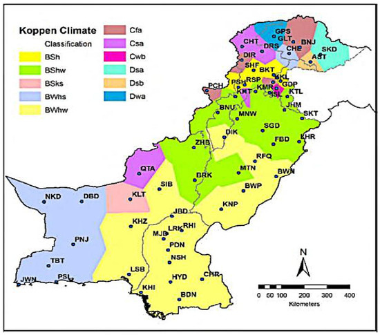
Figure 2.
Pakistan climate classification map based on the Köppen climate classification system showing the spatial distribution of 12 Köppen climate classes with the dominant one being BWhw, followed by the rest [64].
The primary focus of this study is the Indus River basin in Pakistan. The Indus River basin, which is ranked as one of the mightiest basins of the world, covers areas of Afghanistan, China, Pakistan, and India. Pakistan contributes 56% of the total area of the Indus basin, which is the largest amongst all the other neighbouring countries [65]. The Indus River basin in Pakistan covers 520,000 km2, which is 65% of the total area of Pakistan [66]. The climatic conditions of the Indus basin features high variability, from subtropical arid and partial arid to moderate subhumid over the plain areas of two provinces, Sindh and Punjab [67]. The historical record shows an annual precipitation in the range of 100–500 mm in the plain areas compared to the highest value of 2000 mm on alpine slopes [67]. Snowfall is the major source of river runoff at higher elevations of almost 2500 m [68].
The main source of revenue generation in the economy of Pakistan is reliant on agriculture, which depends upon the water resources of the Indus River [33]. The increase in population and industrial growth has caused a drop in water availability from 5600 cubic meters in 1947 to 1017 cubic meters per capita in 2015, which is anticipated to further decrease under the existing infrastructure and organizational conditions [69]. The majority of the water demand of Pakistan is fulfilled through the Indus River and its contributing tributaries, for which the primary source of feeding are precipitation and snowmelt in the HKH mountainous region [70].
2.2. Datasets Collection
The research objectives were achieved with the help of the river’s mean annual streamflow data, mean annual precipitation data, mean annual temperature data, and geospatial datasets. Geospatial datasets of the digital elevation model (DEM) were obtained from the USGS website [71]. The Shuttle Radar Topography Mission (SRTM) DEM was downloaded in 30 × 30 m resolution. Similarly, hydroclimatic datasets include data on streamflow, precipitation, air temperature, etc. The annual streamflow data are made available from the Surface Water Hydrology Project of the Water and Power Development Authority (WAPDA) and the Global Runoff Data Centre (GRDC). A summary of the data that provides resolution (temporal and spatial) and sources of the data is given in Table 1. Based on the available record, the mean annual streamflow data was acquired for different durations at different stations from 1963 to 2009. In this study, 86 stations were chosen across different rivers, keeping in mind the maximum data availability at a particular flow station. The flow station locations are the outlets of catchments. The details of all these catchments along the different rivers of the study area are given in Appendix A of the manuscript. The datasets of annual precipitation and temperature were acquired from the Pakistan Meteorological Department (PMD). Precipitation data were obtained from 47 meteorological stations, while temperature data—from 34 stations within the study period, i.e., in 1963–2009. For precipitation, every catchment was to have at least one precipitation station within its boundaries contributing to Thiessen weighting at a distance of not more than 200 km in plain areas and 150 km in hilly areas [72], although for the majority of the catchments, the distance is less than 100 km from the precipitation station. For temperature data, in plain areas, every catchment was to have at least one temperature gauging station at a distance of 300 km in the vicinity of the catchment boundary contributing to Thiessen weighting [72]. Again, here, for the majority of the catchments, the distance is less than 100 km from the temperature station because the data of all the 34 temperature stations were acquired at the same weather stations at which the precipitation data were acquired.

Table 1.
Summary table indicating data resolution (temporal and spatial) and sources of the data.
2.3. Data Preparation
The annual mean values of streamflow for the available record at each catchment outlet were computed. Similarly, the annual mean values of precipitation and temperature were calculated for all the selected stations and are given in Table A2 of Appendix A.
These values were arranged in a proper format and set ready for the application of a suitable interpolation technique in ArcGIS. The ArcGIS 10.2 platform provides several interpolation techniques that can be used for interpolating climate variables. Many researchers utilized different interpolation techniques for different climate parameters [23,40,48]. For this study, we estimated the basin-averaged precipitation by applying the Thiessen polygon method to the subbasin [71,72,73,74,75,76], whereas an inverse distance-weighted (IDW) model was adopted for the interpolation of both precipitation and temperature elasticity data in ArcGIS 10.2. The interpolated annual mean time series values of precipitation and temperature were extracted for the all the 86 catchments within the study period of 1963–2009.
2.4. Data Uncertainty
The streamflow, precipitation, and temperature data were checked for data quality (missing values), which is indicated by −1 or −100 in the available data record for the streamflow, precipitation, and minimum and maximum temperature values. For this study, the historic record showed that the found missing values in each month of an individual year were fewer than 15 at all the stations. These missing values were linearly interpolated to all such stations [23]. Thus, for this study, it is believed that the influence of time series inhomogeneity on the results was very meagre.
2.5. Methods
In this study, precipitation elasticity of the streamflow was calculated analytically by using long-term hydroclimatic datasets of streamflow, air temperature, and precipitation. Here, we applied the NP bivariate elasticity model, the multivariate NP analysis model, and the multivariate DL analysis model for the estimation of elasticity through NP estimator ɛp.
2.5.1. NP (NP) Bivariate Model
The NP bivariate elasticity model of Sankarasubramanian et al. (2001) [28] was used for the determination of precipitation elasticity in all the 86 catchments. The NP bivariate model for streamflow elasticity is given below.
In Equation (2), variables P and Q are quite general and can be used as instantaneous, monthly, or annual values [77,78,79]. In this study, the mean annual values of streamflow Q and precipitation P for the estimation of were utilized. Where and are the long-term historical means of time data series of the annual mean values of precipitation P and streamflow Q, respectively, at a particular catchment outlet. Precipitation elasticity is estimated for each set of and for an individual year in the annual time series data. The median value of all the calculated elasticity values of the available historic record at a particular catchment outlet is NP precipitation elasticity . The main advantage of this relation is nonparametric and it has low biasness so this is the major advantage of this relationship.
2.5.2. Multivariate NP Analysis Model
Multivariate NP analysis calculates multiple “factor” elasticities in the form of regression coefficients as a result of the multivariate regression model. The multivariate function describes the mutual relationship within climatic variables (precipitation, temperature, humidity, land use, etc.) and streamflow Qi (i indicates the mean flow) [39]. This can be expressed for precipitation and temperature elasticity mathematically in the form of the following equation:
The NP multivariate model is developed by using the chain rule on Equation (3) and supposing that an absolute change in streamflow Q is a linear combination of an absolute change in precipitation P and temperature T.
Inserting the absolute change in every term of Equation (4) for their difference from the mean value, we get the following:
On rearrangement of Equation (5) we get the following:
Applying the definition of elasticity to Equation (6), we can substitute the corresponding elasticity estimator for precipitation and temperature as follows:
In Equation (7), and gives the mean “factor” elasticities of streamflow Q, where and are the long-term historical means of the time series data of the annual mean values of streamflow Q, precipitation P, and temperature T, respectively. Precipitation elasticity and temperature elasticity were obtained as coefficients of the ordinary least squares (OLS) regression. The OLS regression was performed on the values obtained from each set of , , and , for one complete year time t in the time series data. During calculations of regressions, the intercept term was put unadjusted, i.e., the intercept term was taken as zero.
2.5.3. Multivariate DL Analysis Model
The multivariate DL analysis model is also employed in order to get a comparison of the precipitation elasticities obtained through different models and seeks a conclusion as to which model is the most suitable. A more recent study [39] evaluated the impact of the regional factor on streamflow Q by utilizing multivariate regression analysis. It was assumed that the effect of this regional factor on streamflow Q is a dimensionless indicator and so can be marked as factor elasticity of streamflow as follows:
In Equation (8), shows the j factor (climate variable, i.e., precipitation and temperature in our case) that influences streamflow Q, where represents a ratio of proportional change in streamflow to proportional change in . Considering the functional form of Equation (3), we modified the equation introduced by Tsai [39] for evaluating the precipitation elasticity of streamflow as follows:
Taking logarithm of both sides of Equation (9), we get the following:
where in Equation (8) is equal to the precipitation elasticity of streamflow and is equal to temperature elasticity . The values of and were estimated as coefficients of the ordinary least squares (OLS) regression analysis that is performed on the values obtained for each set of Log, Log, and Log for one complete year time t in the time series data. During calculations of regressions, the intercept term was put unadjusted, i.e., the intercept term was taken as zero.
3. Results
3.1. Precipitation Elasticity and Different Models
Precipitation elasticity was calculated using all the three models as mentioned in the methodology section. It was observed that for Sankarasubramanian’s NP bivariate elasticity model, the values were observed in the range from −1.8 to +3.5 with a positive value for 77 catchments and a negative value for nine catchments. The multivariate NP analysis model resulted in values within the range of −2.8 to +3.7 with 74 positive catchments and 12 negative catchments. Similarly, the multivariate DL analysis model estimated the values within the range from −2.7 to +3.9, with 76 positive catchments and 10 negative catchments.
Two-dimensional (2D) line plots were also produced for the models stated above so as to give us a better understanding of the different precipitation elasticity models (Figure 3). It can be seen from Figure 3 that precipitation elasticity of all the 86 catchments (at their outlets) are almost the same for the three employed models, i.e., the values closely matched one another at the majority of the stations.
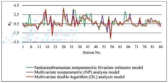
Figure 3.
Precipitation elasticity using the three different models.
Furthermore, nearly all the three employed models showed homogeneity in estimating positive and negative elasticity values in the majority of the catchments. For all the three models, the estimated elasticity values are in the range of 0.1–3.5 for over 70–75% of the catchments. It means that 10% change causes 10–35% change in streamflow for over 70–75% of the catchments. The elasticity estimates of our study were in line with other recent studies that had been conducted on streamflow sensitivity analysis in response to precipitation elasticity for a few subbasins situated within our study area [74,75]. The results of our study are very similar to their findings, for example, Shah et al. (2021) found that 10% variation in precipitation produces 12–20% change in streamflow in six major rivers situated in Khyber Pakhtunkhwa province of Pakistan [74], while in our case, 10% change caused 10–35% change in streamflow for over 75% of the catchments. The spatial spot variation of precipitation elasticity in all the 86 catchments at their outlets is presented in Figure 4 which further clarifies the scenarios through specifying ranges for precipitation elasticity for all the three employed models.
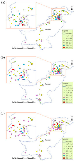
Figure 4.
Precipitation elasticity of the streamflow: (a) NP bivariate model, (b) multivariate NP model, (c) multivariate DL model.
Pakistan is a country with complex topography where precipitation has a high degree of spatiotemporal unpredictability and precipitation elasticity estimates are of variable nature, lacking a clear trend. In general, catchments in the UIB are less sensitive to precipitation elasticity ( ≤ 0.5) because the precipitation in this area is usually in the form of snow, and so the proportion of rainfall contribution to the streamflow within this area is too meagre. On the other hand, elasticity values are relatively higher ( = 0.1–3) near the federal capital territory and the boundary between Khyber Pakhtunkhwa and Punjab provinces as these areas usually receive more rainfall annually. Similarly, the southern part of Pakistan has moderate elasticity ( = 0.1–1) with a few exceptions of high-elasticity catchments.
In order to get an idea of data spread and further elaborate the comparison of the three analytical models for the estimation of precipitation elasticity, we applied statistical tools, i.e., the mean (Figure 5a) and the median (Figure 5b) to the data values of . The mean and median values suggest that all the three models almost equally estimated the precipitation elasticity values.
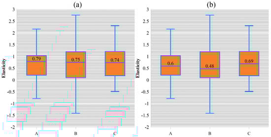
Figure 5.
(a) Boxplots of the mean values of precipitation elasticity, (b) boxplots of the median values of precipitation elasticity. Boxplot A: Sankarasubramanian’s bivariate model, boxplot B: multivariate NP analysis model, boxplot C: multivariate DL analysis model.
It was observed for all the models that the values for the catchments with a consistent and longer historical record in the northern areas of Pakistan, i.e., the UIB, are generally below 0.5 (except a few stations with a shorter record and misleading results). This is because the precipitation in this area is usually in the form of snow, and thus the precipitation elasticity shows less sensitivity of the streamflow as the proportion of rainfall contribution in the streamflow within this area is too meagre. The negative values were observed for stations with a relatively shorter data span (10 or less than 10 years, which is evident from Table A3 of Appendix A) and limited streamflow anomaly ΔQ. Similarly, for the multivariate regression models the corresponding plots were checked individually during calculation for every catchment and was found that in all cases the linear regression does not give significant results. The negative values of climate elasticity and the same shortcoming of regression analysis for shorter span data is evident from climate elasticity literature [45]. Negative elasticity may also be due to the following: (a) there exist storage reservoirs in the catchments or inter-catchment transfer ahead of the catchment gauge outlet; (b) the averaging period is not long enough, i.e., the rainfall has increased but the water has not yet got to the outlet; (c) evaporation exceeding precipitation (might be due to change in land use in the catchment in terms of afforestation or increased vegetation); (d) erroneous measurement of streamflow, climate variables (e.g., precipitation, temperature, evaporation, etc.) or both.
3.2. Comparison of Multivariate NP Analysis Model and Multivariate DL Model
In order to obtain the statistical solution for investigating the best model, the statistics of the two regressions were checked and compared for identifying the best model. A variety of statistical tests are available to test the results for the goodness of fit for regressions. Tsai (2017) applied adjusted R2, probability plot correlation coefficients (PPCC), and variance inflation factors (VIFs) to assess regression goodness of fit. The adjusted R2 is an indicator of the overall performance of a regression model [39]. In this study, the regression of the two multivariate models, i.e., multivariate NP analysis and multivariate DL models, was tested against their adjusted R2 values as shown in Figure 6a.
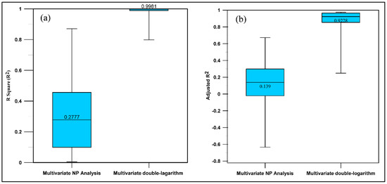
Figure 6.
(a,b) show adjusted R2 and R2 boxplots for the multivariate NP analysis and multivariate double logarithm models, respectively.
Since the values of precipitation elasticity obtained by the regression of the multivariate double logarithm showed higher adjusted values, i.e., higher explanatory power, we can say that for this study, the multivariate DL results were more reliable than the multivariate NP analysis model. This statement is made more worthy by comparison of the boxplots of the R2 values of the multivariate NP analysis and multivariate DL models as shown in Figure 6b. The plot suggests that the values of the multivariate DL model are more concise and are higher, approaching one, which means that it is comparatively more reliable in this case than the multivariate NP model.
3.3. Bivariate Versus Multivariate Analysis
The justification of Sankarasubramanian et al. (2001) [28] regarding the bivariate NP estimator highlights that the median values of precipitation elasticity of the streamflow calculated using an analytical model, i.e., , is more superior compared to a calibrated deterministic hydrological model, though later research on climate elasticity suggested that the result obtained through a single variable does not give true representation of elasticity; rather, it provides misleading information on [48]. It was mentioned that the values using a bivariate model on a single variable do not account for certain other important hydroclimatic factors and catchment characteristics like temperature, land use, humidity, slope, etc. Similarly, it was also found that the regression analysis that includes temperature improves the coefficient of determination (R2) [40]. Since all the subsequent research based on multivariate models suggests that multivariate models are more reliable than bivariate elasticity models [39,42,48,73,74,75,76,77,78,79,80,81,82], it is believed that the multivariate elasticity results of our study are more authentic than the bivariate elasticity results, although there is very small difference between the results as discussed in Section 3.1 above.
3.4. Consequences of Instability Precipitation Elasticity
This section discusses the correlations of the three different analytical models, i.e., the NP bivariate elasticity model, the multivariate NP analysis model, and the multivariate DL model of precipitation elasticity against the catchment and hydroclimatic characteristics.
3.4.1. Precipitation Elasticity and Length of the Available Historical Record
Overall, no significant trend was observed; it can be seen from Figure 7 that in all the three models, negative and outlier behaviour of the precipitation elasticity values was obtained where the historical record was equal to or shorter than 10 years.

Figure 7.
Precipitation elasticity εp and length of study plots: (a) NP bivariate model; (b) multivariate NP analysis model; (c) multivariate DL model.
Although negative elasticity values were also seen for few catchments where the available length of record was quite larger, their values were very small, near zero, and thus were not significant. The possibility of negative values of elasticity in the estimation of precipitation or temperature elasticity indicates that streamflow decreases with an increase in precipitation or temperature [40,41,45].
3.4.2. Precipitation Elasticity and Catchment Area
The catchment areas of 80% of the catchments (79 out of the 86 catchments) are less than 25,000 square km, which is evident in Figure 8. Moreover, it is depicted in the plots that elasticity shows a strong relationship with the catchment area. In all the three models, the elasticity values were found higher for smaller catchment areas compared to the larger catchment areas. This means that for smaller catchments, runoff and snowmelt water takes less time to reach the catchment outlets and thus results in higher elasticity values. Conversely, the elasticity values of larger catchment areas show relatively smaller values. This might be due to the losses caused in terms of evaporation, local reservoirs (ponds, lakes, etc.), and vegetation.

Figure 8.
Precipitation elasticity vs. catchment area plots: (a) NP bivariate model; (b) multivariate NP analysis model; (c) multivariate DL model.
3.4.3. Precipitation Elasticity and Mean Annual Temperature
Logically, there exists a dual relationship between precipitation elasticity and temperature. When temperature increases, evaporation increases, which causes a decrease in runoff water to join the streamflow. On the other hand, the situation is opposite in snow and glacier regions where an increase in temperature causes an increase in runoff and snowmelt and thus boosts the streamflow. The scatterplots in Figure 9 show that there exists relatively lower precipitation elasticity in cold areas where the mean annual temperature is lower because of the existence of glaciers and snowfall as the main source of precipitation [28]. The lower elasticity values in cold areas are also because of less energy available for snow melting [72]. Similarly, an increasing trend of elasticity values was seen from 15 to 22 °C, followed by a decreasing trend (southern part) where the higher temperature causes a reduction in the streamflow due to evaporation.
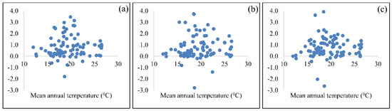
Figure 9.
Precipitation elasticity vs. the mean annual temperature (°C) plots: (a) NP bivariate model; (b) multivariate NP analysis model; (c) multivariate DL model.
3.4.4. Precipitation Elasticity and Mean Annual Precipitation
It is understood that precipitation has a direct impact on streamflow sensitivity and is without any doubt the primary source of river streamflow. The same phenomenon was observed when plots showing the relationship of precipitation elasticity and the mean annual precipitation were produced as shown in Figure 10a–c.
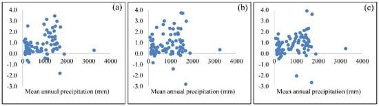
Figure 10.
Precipitation elasticity vs. the mean annual precipitation (mm) plots: (a) NP bivariate model; (b) multivariate NP analysis model; (c) multivariate DL model.
It is visible from the plots that precipitation elasticity showed a relatively higher sensitivity in an increasing trend with an increase in the mean annual precipitation. Although some of the catchments in northern areas showed smaller elasticity values in spite of having a higher mean annual precipitation, this is because the precipitation usually occurs in the form of snow or accumulated snow which usually retains water and does not directly contribute to the streamflow.
3.4.5. Precipitation Elasticity and Mean Annual Streamflow
The mean annual streamflow is dependent on several catchment characteristics like catchment’s slope, terrain, size, shape, altitude, vegetation, land use, etc. Similarly, rainfall intensity, frequency, distribution, and air temperature also significantly affect streamflow, and thus precipitation elasticity . The plots shown in Figure 11 demonstrate a clear understanding of the probable relation of precipitation elasticity and the mean annual streamflow. It is obvious from the plots that relatively higher elasticity values were found in the catchments with lower mean annual flows. The values are generally lower than 1.0 where the streamflow is higher [72]. Higher values were mostly found for smaller catchments where runoff water reaches the gauging station faster. As a result, the streamflow sensitivity becomes high due to less time of concentration and smaller losses in the form of infiltration, inundation, interception, evaporation, etc.
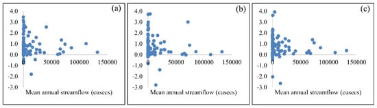
Figure 11.
Precipitation elasticity vs. the mean annual streamflow (cusecs) plots: (a) NP bivariate model; (b) multivariate NP analysis model; (c) multivariate DL model.
3.4.6. Precipitation Elasticity and Altitude
The altitude is an important factor in precipitation elasticity and sensitivity of the streamflow as precipitation patterns and air temperature substantially vary with the altitude of a given region. The plots presented in Figure 12 reveal that the values initially increased with altitude and reached the highest level at an altitude of 250–1000 m because precipitation is more likely at higher altitudes due to a higher chance of lower temperature and more condensation [28,72]. With a further increase in altitude, the values follow a declining trend, which is an indicator of snow and glacier zones in the northern parts of Pakistan, particularly the UIB.
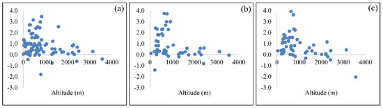
Figure 12.
Precipitation elasticity vs. altitude (m) plots: (a) NP bivariate model; (b) multivariate NP analysis model; (c) multivariate DL model.
3.4.7. Precipitation Elasticity and Spatial Trends
It was observed from the plots in Figure 13 that longitude-wise, higher elasticity values were found between 70 and 75 decimal degrees, while latitude-wise, higher elasticity values were found between 32 and 36 decimal degrees.
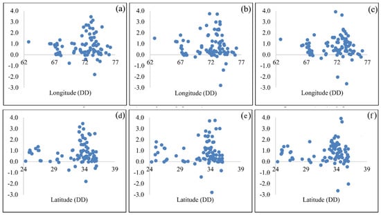
Figure 13.
Precipitation elasticity vs. longitude and latitude plots: (a,d) NP bivariate model; (b,e) multivariate NP analysis model; (c,f) multivariate DL model.
This spatial trend of precipitation elasticity is further elaborated by interpolating the elasticity values by using the inverse distance weighting (IDW) technique for the NP bivariate model, the multivariate NP analysis model, and the multivariate DL model in Figure 14a–c, respectively.
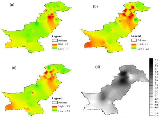
Figure 14.
Spatial trend of εp: (a) NP bivariate model, (b) multivariate NP analysis model, (c) multivariate DL model, (d) monsoon precipitation trend (Hanif et al., 2013 [80]).
The streamflow sensitivity obtained using the three employed models in this study is reinforced by the almost matching results of another study for Pakistan [80] with approximately the same study period, i.e., 1951–2010 (Figure 14d).
Almost 60% of the total mean annual water is contributed by headwaters of the Indus basin, out of which approximately 80% of the annual total water joins the system from June to September every year, which is called the monsoon season in Pakistan [70].
By comparing the precipitation elasticity maps in Figure 14a–c with the monsoon rainfall trend map as shown in Figure 14d (Hanif et al. (2013) [80]), a close resemblance was observed among the areas of higher precipitation elasticity and the areas with higher monsoon rainfall. Since rainfall is the most important and governing climate parameter that contributes to river flows, it is more likely that areas receiving more precipitation will possesses higher streamflow sensitivity due to greater runoff generation and might yield high . The results of this study show higher sensitivity in areas where the monsoon rainfall intensity is higher and vice versa which proves the authenticity of this study and elasticity models.
3.5. Temperature Elasticity
In addition to precipitation elasticity, temperature elasticity was also evaluated using three models i.e., Sankarasubramanian’s NP bivariate model, the multivariate NP analysis model, and the multivariate DL model to check the response of the streamflow to the mean temperature. Temperature elasticity estimates for all the three models are shown in Figure 15.
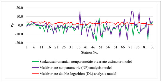
Figure 15.
Comparison chart showing temperature elasticity as obtained using Sankarasubramanian’s NP model, the multivariate NP analysis model, and the multivariate NP DL model.
It was observed that ranged between −17.9 and +16 for Sankarasubramanian’s NP bivariate model and the multivariate NP analysis model, while for the multivariate double logarithm model, the values were in the range of +2.3–+4.7. In the case of temperature elasticity, there exist large variations of the maximum and minimum values between the multivariate DL model and the other two models, i.e., Sankarasubramanian’s NP bivariate model and the multivariate NP analysis model. The linear trend in the values of the double logarithm was due to the log transformation behaviour which smoothened the variation in regression. Sankarasubramanian’s NP bivariate model and the multivariate NP analysis model showed relatively similar results at the majority of the catchments.
The estimations of Sankarasubramanian’s NP bivariate elasticity model and the multivariate NP analysis model suggest that about 65% of the catchment showed negative values of . This means that the increase in temperature caused a decrease in the streamflow, which is logical as the increase in temperature accelerates the evaporation process and results in a decreased streamflow. Overall, the values obtained using all the three models, which are comprised ofillogical and unrealistic values. Thus, the results of temperature are not reliable and are misleading. Furthermore, the existing literature also suggests that there is no significant impact of residual temperature on the streamflow compared to the direct and much more significant impact of precipitation on the streamflow, all because of the opposite correlation between precipitation and temperature [76,77,78,79,80,81,82].
3.6. Recommendations Regarding Water Management and Policy-Making Based on Elasticity
Although in this study only a relatively straightforward targeting approach was undertaken, the results of the various comparisons made in the study point to the daunting challenges that will exist in the future for developing and implementing watershed management plans that are effective in improving water management practices in stream systems throughout the country. Generally, the elasticity value is an indicator of sensitivity of the streamflow. The higher the elasticity value, the higher the sensitivity, and vice versa. Consequently, catchments having higher elasticity values are prone to aggressive climate events in the form of flash floods, and thus the existing infrastructure needs proper design to protect the inhabitants and flora and fauna of the catchments against the expected flood risks. Similarly, a lower elasticity value is an indicator of drought, and policymakers need to adopt necessary actions for coping with the drought situation through water management techniques. The smaller catchments were found to be more sensitive, with higher elasticity, and so the water supply schemes and cultivable agricultural land are more susceptible to flooding events and calamities; thus, best management practices must be ensured in all such areas.
4. Conclusions
The design, planning, and management of various preliminary hydrological studies require annual runoff volume for watersheds. For such purposes, regional methods that link streamflow to climate characteristics can offer a better solution. This study presents the estimates of precipitation elasticity of the streamflow in 86 catchments of Pakistan using the NP bivariate model, the multivariate NP analysis model, and the multivariate DL analysis model. Based on the results of statistical tests, it was concluded that the higher explanatory power of the multivariate DL model suggests that it gave more reliable values of precipitation elasticity compared to Sankarasubramanian’s NP bivariate elasticity model and the multivariate NP analysis model within the study area.
Additionally, all the employed models showed relatively similar results indicating elasticity in the range of 0.1–3.5 (observed in almost 70% of the total catchments using the multivariate NP analysis model and 75% of the catchments for both Sankarasubramanian’s NP bivariate elasticity model and the multivariate double logarithm model). Precipitation elasticity of the streamflow is defined as the percentage of change in the mean annual streamflow for a given percentage change in the mean annual precipitation. This means that a 1% change in precipitation with respect to long-term historic mean annual precipitation will change the streamflow by %, i.e., by 0.1–3.5% in our case. Similarly, if this change is assumed, a 10% change with respect to long-term mean annual precipitation will amplify the streamflow by 1–35%.
The study further revealed that the elasticity estimates of the catchments having a shorter historical record, i.e., usually less than 10 years, yielded misleading values and showed an outlier behaviour, i.e., either overestimating or underestimating the elasticity. Similarly, it was found that is relatively higher at an altitude ranging between 250 and 1000 m and at the catchments where the mean annual temperature is relatively high, i.e., from 15 °C to 22 °C. The longitudinal and latitudinal pattern of showed high elasticity in the range from 70 to 75 and from 32 to 36 decimal degrees, respectively. Furthermore, the precipitation elasticity was found to have a direct relationship with the mean annual precipitation and an inverse relationship with the catchment areas. The study also found that the temperature elasticity values in the majority of the catchment areas were not significant and showed outlier or unrealistic behaviour, and thus the results of temperature elasticity cannot be significantly utilized in analysing streamflow sensitivity; however, it improved the results of precipitation elasticity in multivariate approaches.
Author Contributions
Conceptualization, Z.K., F.A.K. and A.U.K.; Data curation, I.H. and A.K.; Formal analysis, P.K., A.D. and K.R.; Funding acquisition, I.H., P.K. and K.R.; Investigation, I.H.; Methodology, A.K., L.A.S. and J.K.; Project administration, I.H. and P.K.; Resources, I.H. and P.K.; Software, I.H. and Y.I.B.; Supervision, F.A.K., A.U.K., I.H. and A.D.; Validation, Y.I.B.; Visualization, J.K.; Writing—original draft, Z.K.; Writing—review & editing, Z.K., A.U.K. and I.H. All authors have read and agreed to the published version of the manuscript.
Funding
This research received no external funding.
Institutional Review Board Statement
Not applicable.
Informed Consent Statement
Not applicable.
Data Availability Statement
Geospatial datasets of the digital elevation model (DEM) can be freely obtained from the USGS website [71]. Similarly, hydroclimatic datasets include data of streamflow, precipitation, air temperature, etc. The precipitation and temperature datasets are available from the Pakistan Meteorological Department (PMD) on payment of specified data charges. The annual streamflow data are made available by the Surface Water Hydrology Project of the Water and Power Development Authority (WAPDA) on payment of specified data charges. Streamflow data can also be freely downloaded from the Global Runoff Data Centre’s (GRDC) website, https://www.bafg.de/GRDC/EN/Home/homepage_node.html (accessed on 31 December 2021).
Acknowledgments
The authors would like to express gratitude toward Almighty Allah, the wellspring of all learning and knowledge inside and outside our ability to grasp. The authors appreciate the supporting staff and management of the Water and Power Development Authority (WAPDA) and the Pakistan Meteorological Department (PMD) for their help in arranging and providing the required data to us, which really helped out in the accomplishment of this study.
Conflicts of Interest
The authors affirm that there are no conflict of interest regarding the publication of this manuscript. Furthermore, ethical issues, data fabrication, double publication, or submission to any other journal were absolutely put under consideration by the authors. Furthermore, no funding source financed the expenses of this study, and all the expenses of the work was born by the authors on their own.
Appendix A
Table A1.
Complete details of the streamflow monitoring stations.
Table A1.
Complete details of the streamflow monitoring stations.
| Station No. | River and Catchment Outlet Name | X Outlet DD | Y Outlet DD | Standard Elevation (m.a.s.l) | Available Record (yrs) | Catchment (km2) |
|---|---|---|---|---|---|---|
| 1 | Indus River at Kharmong | 76.1834 | 34.9728 | 2436 | 27 | 67,858 |
| 2 | Shyok River at Yugo | 75.9742 | 35.2050 | 2308 | 37 | 33,670 |
| 3 | Shigar River at Shigar | 75.7130 | 35.3993 | 2222 | 14 | 4144 |
| 4 | Indus River at Kachura | 75.4627 | 35.4449 | 2219 | 40 | 112,664 |
| 5 | Indus River near Gunji Bridge | 74.8102 | 35.7148 | 1591 | 7 | 785 |
| 6 | Hunza River at Dainyor Bridge | 74.2933 | 35.9458 | 2028 | 40 | 13,157 |
| 7 | Gilgit River at Gilgit | 74.1821 | 35.9452 | 3140 | 40 | 12,095 |
| 8 | Gilgit River at Alam Bridge | 74.5710 | 35.7816 | 1365 | 40 | 26,159 |
| 9 | Indus River at Partab Bridge | 74.6359 | 35.6913 | 1298 | 31 | 142,708 |
| 10 | Sai Nallah at Urkakai | 74.4870 | 35.7913 | 2421 | 8 | 554 |
| 11 | Indus River near Bunji Bridge | 74.6193 | 35.6102 | 1305 | 11 | 97 |
| 12 | Astore River at Doyian | 74.7380 | 35.5297 | 1668 | 36 | 4040 |
| 13 | Indus River at Raikot | 74.1948 | 35.4058 | 1052 | 4 | 385 |
| 14 | Indus River at Shatial Bridge | 73.4830 | 35.5409 | 922 | 25 | 129,499 |
| 15 | Gorbund River at Kabora | 72.8292 | 34.9242 | 749 | 30 | 635 |
| 16 | Indus River at Bisham Qila | 72.8902 | 34.8819 | 638 | 39 | 162,392 |
| 17 | Brandu River near Dagger | 72.5254 | 34.4902 | 669 | 36 | 598 |
| 18 | Siran River near Phulra | 73.0710 | 34.3079 | 829 | 37 | 1057 |
| 19 | Golan Gol River at Bubka | 72.1346 | 35.9687 | 3567 | 6 | 541 |
| 20 | Golan Gol River at Mastuj Bridge | 72.0148 | 35.9234 | 2270 | 12 | 518 |
| 21 | Siran River near Thapla | 72.8333 | 34.1229 | 430 | 9 | 2797 |
| 22 | Chitral River at Chitral | 71.7873 | 35.8339 | 1471 | 42 | 11,396 |
| 23 | Kabul River at Warsak | 71.2482 | 34.2581 | 650 | 9 | 67,340 |
| 24 | Swat River near Kalam | 72.6033 | 35.3647 | 1748 | 43 | 2020 |
| 25 | Swat River at Chakdara | 72.0369 | 34.6741 | 726 | 43 | 5776 |
| 26 | Panjkora River at Zulam Bridge | 71.7865 | 34.7594 | 645 | 8 | 597 |
| 27 | Swat River at Munda Dam | 71.5119 | 34.4079 | 580 | 8 | 392 |
| 28 | Bara River at Jhansi Post | 71.2955 | 33.8325 | 707 | 43 | 1847 |
| 29 | Kabul at Nowshehra | 71.8536 | 33.9839 | 328 | 43 | 88,578 |
| 30 | Kalpani River near Risalpur | 72.0654 | 34.0488 | 294 | 8 | 722 |
| 31 | Indus River at Khairabad/Mandori | 72.2286 | 33.8317 | 291 | 36 | 264,179 |
| 32 | Haro River at Dhartian | 73.0497 | 33.8574 | 773 | 7 | 621 |
| 33 | Nilan Kass River at Najaf Pur | 73.0037 | 33.7370 | 830 | 7 | 57 |
| 34 | Haro River near Khanpur | 72.8911 | 33.7899 | 539 | 28 | 777 |
| 35 | Haro River near Sanjawal | 72.3814 | 33.7483 | 313 | 9 | 1800 |
| 36 | Haro River at Gariala | 72.2168 | 33.7653 | 271 | 37 | 3056 |
| 37 | Kohat Toi at Jarma Weir | 71.5844 | 33.4278 | 350 | 6 | 1541 |
| 38 | Soan River at Chirah | 73.2995 | 33.6505 | 576 | 43 | 326 |
| 39 | Ling River near Kahuta | 73.3203 | 33.5603 | 533 | 9 | 153 |
| 40 | Soan at Gorakh Pur Bridge | 72.5949 | 33.1650 | 323 | 12 | 326 |
| 41 | Soan River near Rawalpindi | 73.0615 | 33.4915 | 399 | 31 | 1683 |
| 42 | Sil River near Chahan | 72.7874 | 33.3643 | 361 | 43 | 241 |
| 43 | Soan River at Dhok Pathan | 72.2099 | 33.1237 | 283 | 42 | 6475 |
| 44 | Indus River at Massan | 71.4547 | 32.8880 | 199 | 33 | 287,489 |
| 45 | Kurram River at Thal | 70.4857 | 33.4261 | 806 | 39 | 5543 |
| 46 | Tochi River at Tangi Post | 70.4930 | 32.8734 | 381 | 25 | 5128 |
| 47 | Tank Zam near Jandola | 70.1767 | 32.3073 | 604 | 23 | 2176 |
| 48 | Zhob River at Sherik Weir | 69.4283 | 31.4473 | 1304 | 10 | 10,360 |
| 49 | Gomal River at Khajurikach | 69.8628 | 32.1003 | 729 | 22 | 29,008 |
| 50 | Gomal River at Kot Murtaza | 70.2454 | 32.0227 | 252 | 37 | 36,001 |
| 51 | Daraban Zam at Zam Tower | 70.2295 | 31.7817 | 279 | 16 | 1062 |
| 52 | Indus River at Dadu Moro Bridge | 67.8856 | 26.7453 | 45 | 25 | 32,634 |
| 53 | Chenab River at Alexandria Bridge | 74.0584 | 32.4895 | 220 | 6 | 13,792 |
| 54 | Jhelum River at Chinari | 73.8580 | 34.1309 | 25 | 13,546 | |
| 55 | Jehlum at Majohi | 73.5958 | 34.2481 | 796 | 5 | 14,292 |
| 56 | Jhelum River at Domel | 73.5140 | 34.3296 | 714 | 29 | 14,504 |
| 57 | Neelum River at Dhundnial | 74.1367 | 34.7322 | 1815 | 10 | 5439 |
| 58 | Neelum at Nosheri | 73.8377 | 34.5566 | 1336 | 17 | 6809 |
| 59 | Kishanganga/Neelum at Muzaffarabad | 73.4854 | 34.4148 | 760 | 42 | 7278 |
| 60 | Kunhar River at Naran | 73.5003 | 34.7227 | 2508 | 41 | 1036 |
| 61 | Kunhar River at Talhata Bridge | 73.3540 | 34.5547 | 992 | 12 | 2354 |
| 62 | Kunhar River at Garhi Habibullah | 73.3873 | 34.3986 | 820 | 30 | 2383 |
| 63 | Jhelum River at Kohala | 73.4947 | 34.1295 | 586 | 29 | 248,898 |
| 64 | Bishan Daur Kas near Missa | 73.3203 | 33.2136 | 452 | 7 | 150 |
| 65 | Jehlum at Chattar Klass | 73.5119 | 34.0241 | 654 | 11 | 24,700 |
| 66 | Jhelum River at Azad Pattan | 73.5616 | 33.7828 | 506 | 28 | 26,485 |
| 67 | Kanshi River near Palote | 73.5156 | 33.2329 | 430 | 35 | 1111 |
| 68 | Poonch River near Kotli | 73.8967 | 33.5121 | 602 | 42 | 3237 |
| 69 | Jhelum River at Mangla Cableway | 73.6554 | 33.1480 | 335 | 19 | 33,411 |
| 70 | Khost River at Chappar Rift | 67.4999 | 30.3269 | 1431 | 22 | 1191 |
| 71 | Beji River at Babar Kach | 68.0450 | 29.7867 | 308 | 10 | 4558 |
| 72 | Nari River near Sibi | 67.8473 | 29.5587 | 134 | 10 | 22,559 |
| 73 | Chakkar River at Talli Tangi | 68.2746 | 29.6186 | 469 | 5 | 1484 |
| 74 | Bolan River at Kundlani Bridge | 67.5722 | 29.5004 | 188 | 10 | 4040 |
| 75 | Mula River at Naulang | 67.2708 | 28.3772 | 244 | 9 | 8599 |
| 76 | Gaj Nai near Jubble | 67.2420 | 26.8639 | 179 | 5 | 6863 |
| 77 | Indus River near Sehwan | 67.8971 | 26.3953 | 25 | 15 | 1250 |
| 78 | Dasht River at Mirani Dam Site | 62.7529 | 25.9970 | 68 | 5 | 22,533 |
| 79 | Hub River at Karpasaniwat | 67.1635 | 25.3759 | 96 | 14 | 1430 |
| 80 | Hub River at Bund Murad Khan | 67.0292 | 25.1167 | 47 | 10 | 9428 |
| 81 | Porali River at Sinchi Bent | 66.4370 | 26.5235 | 340 | 16 | 4040 |
| 82 | Kud River near Mai Gundrani | 66.2285 | 26.4235 | 232 | 14 | 2085 |
| 83 | Khadeji River at Super Highway | 67.4502 | 25.0300 | 170 | 13 | 567 |
| 84 | Liyari River at Super Highway Bridge | 67.0950 | 24.9397 | 33 | 5 | 207 |
| 85 | Malir River at Super Highway Bridge | 67.4045 | 25.0486 | 110 | 12 | 2235 |
| 86 | Malir River at National Highway | 67.5788 | 24.3406 | 2 | 5 | 2176 |
Table A2.
List of the meteorological stations for the precipitation and temperature datasets.
Table A2.
List of the meteorological stations for the precipitation and temperature datasets.
| S. No | Station Name | X (DD) | Y (DD) | Elevation (a.m.s.l) | Available Dataset |
|---|---|---|---|---|---|
| 1 | Astore | 74.9000 | 35.3333 | 2168.0 | Precipitation, temperature |
| 2 | Bunji | 74.6333 | 35.6667 | 1372.0 | Precipitation, temperature |
| 3 | Chillas | 74.1000 | 35.4167 | 1250 | Precipitation, temperature |
| 4 | Skardu (AP) | 75.6833 | 35.3000 | 2317.0 | Precipitation, temperature |
| 5 | Gilgit | 74.3333 | 35.9167 | 1460.0 | Precipitation, temperature |
| 6 | Dir | 71.8500 | 35.2000 | 1375.0 | Precipitation, temperature |
| 7 | Darosh | 71.7833 | 35.5667 | 1463.9 | Precipitation, temperature |
| 8 | Balakot | 72.3500 | 34.5500 | 995.4 | Precipitation, temperature |
| 9 | Cherat | 71.5500 | 33.8167 | 1372.0 | Precipitation, temperature |
| 10 | Dalbandin | 64.4000 | 28.8833 | 848.0 | Precipitation, temperature |
| 11 | D.I. Khan | 70.8667 | 31.9167 | 172.3 | Precipitation, temperature |
| 12 | Hyderabad | 68.4167 | 25.3833 | 28.0 | Precipitation, temperature |
| 13 | Jacobabad | 68.4667 | 28.3000 | 55.0 | Precipitation, temperature |
| 14 | Jhelum | 73.7333 | 32.9333 | 287.2 | Precipitation, temperature |
| 15 | Kakul | 73.2500 | 34.1833 | 1308.0 | Precipitation, temperature |
| 16 | Karachi (AP) | 66.9333 | 24.9000 | 22.0 | Precipitation, temperature |
| 17 | Kohat | 71.4330 | 33.5670 | 512.0 | Precipitation, temperature |
| 18 | Kotli | 73.9000 | 33.5167 | 614.0 | Precipitation, temperature |
| 19 | Muzaffarabad | 73.4833 | 34.3667 | 838.0 | Precipitation, temperature |
| 20 | Peshawar | 71.5600 | 33.87200 | 327.0 | Precipitation, temperature |
| 21 | Quetta | 66.9500 | 30.1833 | 1626.0 | Precipitation, temperature |
| 22 | Zhob | 69.4667 | 31.3500 | 1405.0 | Precipitation, temperature |
| 23 | Parachinar | 70.0833 | 33.8666 | 1725.0 | Precipitation, temperature |
| 24 | Bahawalpur | 71.7833 | 29.3333 | 110.0 | Precipitation, temperature |
| 25 | Bahawalnagar | 29.9500 | 68.9000 | 163.0 | Precipitation, temperature |
| 26 | Faisalabad | 73.1333 | 31.4333 | 185.6 | Precipitation, temperature |
| 27 | Gupis | 73.4000 | 36.1667 | 2156.0 | Precipitation, temperature |
| 28 | Islamabad | 73.1000 | 33.6170 | 508.0 | Precipitation, temperature |
| 29 | Khanpur | 70.6830 | 28.650 | 88.4 | Precipitation, temperature |
| 30 | Lahore (PBO) | 74.3333 | 31.5500 | 214.0 | Precipitation, temperature |
| 31 | Mianwali | 71.5170 | 32.5490 | 212.0 | Precipitation, temperature |
| 32 | Multan | 71.4333 | 30.2000 | 122.0 | Precipitation, temperature |
| 33 | Muree | 73.3830 | 33.9170 | 2213.0 | Precipitation, temperature |
| 34 | Sargodha | 72.6667 | 32.0500 | 187.0 | Precipitation, temperature |
| 35 | Sialkot | 74.5333 | 32.5167 | 255.1 | Precipitation, temperature |
| 36 | Mangla | 73.6333 | 33.0667 | 283.3 | Precipitation |
| 37 | Risalpur | 71.9830 | 34.067 | 317 | Precipitation |
| 38 | Saidu | 72.35 | 34.767 | 953 | Precipitation |
| 39 | Bannu | 70.1000 | 33.0000 | 406 | Precipitation |
| 40 | Paddian | 68.1333 | 26.8500 | 46 | Precipitation |
| 41 | Nawab Shah | 68.3667 | 26.2500 | 37 | Precipitation |
| 42 | Panjgur | 64.1000 | 26.9667 | 968 | Precipitation |
| 43 | Jiwani | 61.8000 | 25.0667 | 56 | Precipitation |
| 44 | Sibbi | 67.8833 | 29.5500 | 133 | Precipitation |
| 45 | Nokundi | 62.7500 | 28.8167 | 682 | Precipitation |
| 46 | Badin | 68.9000 | 24.6333 | 9 | Precipitation |
| 47 | Kalat | 66.5833 | 29.0333 | 2015 | Precipitation |
Table A3.
Complete set of the precipitation and temperature elasticity values obtained using three different approaches.
Table A3.
Complete set of the precipitation and temperature elasticity values obtained using three different approaches.
| Precipitation Elasticity | Temperature Elasticity | |||||||
|---|---|---|---|---|---|---|---|---|
| Catchment No. | River and Station Name | Available Record (Years) | Sankarasubramanian’s NP Bivariate Estimator | Multivariate NP Analysis | Multivariate DL Analysis | Sankarasubramanian’s NP Bivariate Estimator | Multivariate NP Analysis | Multivariate DL Analysis |
| 1 | Indus River at Kharmong | 27 | 0.7 | 0.6 | 0.3 | −0.5 | −1.5 | 3.7 |
| 2 | Shyok River at Yugo | 37 | 0.0 | 0.0 | −0.2 | 2.1 | 0.8 | 3.7 |
| 3 | Shigar River at Shigar | 14 | 0.8 | 0.2 | 0.0 | 0.3 | −0.2 | 3.6 |
| 4 | Indus River at Kachura | 40 | 0.2 | 0.2 | 0.1 | 1.5 | 1.4 | 4.2 |
| 5 | Indus River near Gunji Bridge | 7 | 2.5 | 0.2 | 0.3 | 0.4 | 3.0 | 3.8 |
| 6 | Hunza River at Dainyor Bridge | 40 | 0.1 | 0.0 | 0.0 | 2.9 | 3.0 | 3.4 |
| 7 | Gilgit River at Gilgit | 40 | 0.3 | 0.3 | 0.4 | 0.0 | 0.3 | 3.4 |
| 8 | Gilgit River at Alam Bridge | 40 | 0.1 | 0.1 | 0.3 | −0.4 | 1.1 | 3.6 |
| 9 | Indus River at Partab Bridge | 31 | 0.0 | 0.0 | 0.2 | −0.1 | 0.5 | 3.9 |
| 10 | Sai Nallah at Urkakai | 8 | −0.6 | −0.8 | −0.5 | −4.5 | −0.5 | 2.0 |
| 11 | Indus River near Bunji Bridge | 11 | 0.5 | 0.1 | 0.2 | 0.1 | 0.2 | 3.9 |
| 12 | Astore River at Doyian | 36 | 0.5 | 0.6 | 0.9 | −2.1 | −0.2 | 3.2 |
| 13 | Indus River at Raikot | 4 | 1.0 | 0.9 | 1.1 | −7.0 | 0.1 | 4.3 |
| 14 | Indus River at Shatial Bridge | 25 | 0.2 | 3.0 | 1.4 | 0.6 | 3.0 | 3.7 |
| 15 | Gorbund River at Kabora | 30 | 2.4 | 3.0 | 3.6 | −5.9 | −7.9 | 0.3 |
| 16 | Indus River at Bisham Qila | 39 | 0.6 | 0.3 | 0.6 | 0.6 | 0.5 | 3.7 |
| 17 | Brandu River near Dagger | 36 | 0.3 | 0.4 | 0.5 | −5.0 | 0.4 | 1.6 |
| 18 | Siran River near Phulra | 37 | 1.3 | 2.3 | 2.2 | −3.8 | −1.9 | 1.2 |
| 19 | Golan Gol River at Bubka | 6 | −0.4 | −0.1 | −2.0 | −7.8 | −9.3 | 1.5 |
| 20 | Golan Gol River at Mastuj Bridge | 12 | 0.9 | 0.6 | 1.1 | −3.7 | −1.5 | 1.8 |
| 21 | Siran River near Thapla | 9 | 0.4 | 0.3 | 0.7 | −4.0 | −8.0 | 2.1 |
| 22 | Chitral River at Chitral | 42 | 0.2 | 0.1 | 0.6 | 0.4 | 0.6 | 3.1 |
| 23 | Kabul River at Warsak | 9 | 0.5 | 0.4 | 0.8 | −6.8 | −2.9 | 3.3 |
| 24 | Swat River near Kalam | 43 | 0.2 | 0.0 | 0.1 | −0.2 | −0.4 | 2.8 |
| 25 | Swat River at Chakdara | 43 | 0.0 | 0.0 | 0.0 | −0.6 | −0.5 | 3.2 |
| 26 | Panjkora River at Zulam Bridge | 8 | 2.5 | 3.7 | 3.9 | −9.6 | −3.3 | 1.0 |
| 27 | Swat River at Munda Dam | 8 | 1.7 | 1.7 | 1.5 | 1.4 | −0.3 | 2.8 |
| 28 | Bara River at Jhansi Post | 43 | 0.4 | 2.7 | 1.6 | −4.1 | −8.0 | 1.4 |
| 29 | Kabul at Nowshehra | 43 | 0.2 | 0.4 | 0.4 | −0.6 | −1.5 | 3.5 |
| 30 | Kalpani River near Risalpur | 8 | 0.2 | 0.3 | 0.4 | −2.3 | −1.8 | 2.4 |
| 31 | Indus River at Khairabad/Mandori | 36 | 1.0 | 0.0 | 0.2 | −2.5 | −1.6 | 3.9 |
| 32 | Haro River at Dhartian | 7 | 3.0 | 3.7 | 2.3 | 1.7 | −2.6 | 1.0 |
| 33 | Nilan Kass River at Najaf Pur | 7 | 3.5 | −0.2 | −0.2 | −6.6 | −2.5 | 1.3 |
| 34 | Haro River near Khanpur | 28 | 1.5 | 1.9 | 1.5 | −3.9 | −5.2 | 1.2 |
| 35 | Haro River near Sanjawal | 9 | 0.0 | 0.2 | 0.2 | −0.2 | −0.5 | 2.1 |
| 36 | Haro River at Gariala | 37 | 2.2 | 0.8 | 1.1 | −3.6 | −4.5 | 1.9 |
| 37 | Kohat Toi at Jarma Weir | 6 | 0.9 | 1.8 | 1.6 | 15.3 | 16.0 | 1.1 |
| 38 | Soan River at Chirah | 43 | 2.4 | 2.3 | 2.1 | −7.3 | −11.1 | 0.8 |
| 39 | Ling River near Kahuta | 9 | −0.1 | 2.3 | 1.2 | −1.8 | 3.5 | 0.9 |
| 40 | Soan at Gorakh Pur Bridge | 12 | 2.7 | 2.3 | 1.8 | −2.6 | 4.8 | 1.6 |
| 41 | Soan River near Rawalpindi | 31 | 1.5 | 1.8 | 1.5 | 1.7 | −0.7 | 1.6 |
| 42 | Sil River near Chahan | 43 | 1.9 | 1.2 | 1.7 | −2.1 | −12.6 | 0.6 |
| 43 | Soan River at Dhok Pathan | 42 | 2.7 | 1.2 | 1.4 | −3.3 | −4.4 | 2.0 |
| 44 | Indus River at Massan | 33 | 0.2 | 0.3 | 0.4 | 0.4 | −0.6 | 3.7 |
| 45 | Kurram River at Thal | 39 | 0.6 | 0.7 | 0.8 | −6.5 | −6.2 | 2.1 |
| 46 | Tochi River at Tangi Post | 25 | 0.6 | 0.8 | 1.1 | −11.2 | −15.8 | 1.6 |
| 47 | Tank Zam near Jandola | 23 | 0.2 | 0.1 | 0.0 | −9.1 | −3.9 | 1.9 |
| 48 | Zhob River at Sherik Weir | 10 | −0.8 | −0.2 | −0.3 | −17.9 | 5.1 | 1.8 |
| 49 | Gomal River at Khajurikach | 22 | 1.0 | 0.3 | 0.4 | −2.7 | 1.3 | 2.3 |
| 50 | Gomal River at Kot Murtaza | 37 | 1.0 | 2.4 | 1.0 | 8.4 | 5.5 | 2.2 |
| 51 | Daraban Zam at Zam Tower | 16 | 0.3 | 0.2 | 0.1 | −9.5 | −11.6 | 1.3 |
| 52 | Indus River at Dadu Moro Bridge | 25 | 0.1 | 0.1 | 0.3 | −14.8 | −10.3 | 3.5 |
| 53 | Chenab River at Alexandria Bridge | 6 | −0.5 | −1.4 | 0.1 | 1.3 | −6.3 | 3.2 |
| 54 | Jhelum River at Chinari | 25 | 2.1 | 1.3 | 1.7 | −6.2 | −7.0 | 2.4 |
| 55 | Jehlum at Majohi | 5 | −1.8 | −2.8 | −2.7 | −0.9 | 2.3 | 4.7 |
| 56 | Jhelum River at Domel | 29 | 0.9 | 0.8 | 1.1 | −5.0 | −6.5 | 2.6 |
| 57 | Neelum River at Dhundnial | 10 | 0.2 | 1.0 | 0.9 | −1.7 | −2.8 | 3.0 |
| 58 | Neelum at Nosheri | 17 | 1.2 | 1.8 | 1.1 | −10.1 | −11.0 | 2.7 |
| 59 | Kishanganga/Neelum at Muzaffarabad | 42 | 0.9 | 0.5 | 0.8 | −4.1 | −4.4 | 2.7 |
| 60 | Kunhar River at Naran | 41 | 0.3 | 0.1 | 0.5 | −3.4 | −1.9 | 2.3 |
| 61 | Kunhar River at Talhata Bridge | 12 | 0.8 | 0.6 | 1.0 | −4.4 | −3.4 | 0.4 |
| 62 | Kunhar River at Garhi Habibullah | 30 | 0.5 | 0.2 | 0.3 | −0.6 | −1.4 | 2.6 |
| 63 | Jhelum River at Kohala | 29 | 0.4 | 0.5 | 0.7 | −0.7 | −0.1 | 3.3 |
| 64 | Bishan Daur Kas near Missa | 7 | 3.1 | 1.1 | 1.0 | −8.0 | −14.1 | 0.4 |
| 65 | Jehlum at Chattar Klass | 11 | 1.6 | 1.1 | 1.4 | −1.3 | −1.5 | 2.9 |
| 66 | Jhelum River at Azad Pattan | 28 | 1.0 | 1.2 | 1.3 | −1.6 | −1.8 | 3.0 |
| 67 | Kanshi River near Palote | 35 | 1.9 | 2.8 | 1.9 | 1.8 | 7.1 | 1.0 |
| 68 | Poonch River near Kotli | 42 | 0.8 | 0.5 | 0.8 | 0.0 | −4.0 | 2.4 |
| 69 | Jhelum River at Mangla Cableway | 19 | 0.3 | 0.2 | 0.3 | −6.2 | −16.6 | 3.1 |
| 70 | Khost River at Chappar Rift | 22 | 0.5 | 0.0 | 0.5 | 0.3 | 1.2 | 1.1 |
| 71 | Beji River at Babar Kach | 10 | −0.1 | 0.0 | −0.1 | 0.2 | 4.0 | 1.8 |
| 72 | Nari River near Sibi | 10 | 0.2 | 0.0 | 0.1 | 0.6 | 15.9 | 2.0 |
| 73 | Chakkar River at Talli Tangi | 5 | 0.8 | 1.2 | 1.8 | −12.0 | 15.0 | 2.0 |
| 74 | Bolan River at Kundlani Bridge | 10 | 0.2 | 0.1 | 0.2 | −0.8 | −0.5 | 1.5 |
| 75 | Mula River at Naulang | 9 | 0.0 | 0.5 | 0.2 | 0.3 | 1.8 | 1.5 |
| 76 | Gaj Nai near Jubble | 5 | 0.1 | 0.2 | 0.2 | −6.0 | −2.1 | 1.5 |
| 77 | Indus River near Sehwan | 15 | 1.3 | 0.0 | 0.1 | −9.7 | 15.4 | 3.3 |
| 78 | Dasht River at Mirani Dam Site | 5 | 1.2 | 1.5 | 1.4 | −6.3 | −7.0 | 2.4 |
| 79 | Hub River at Karpasaniwat | 14 | 0.7 | 0.8 | 1.3 | −4.6 | −4.8 | 2.1 |
| 80 | Hub River at Bund Murad Khan | 10 | 0.9 | 1.8 | 1.0 | −3.0 | −3.8 | 2.0 |
| 81 | Porali River at Sinchi Bent | 16 | 1.0 | 1.2 | 0.9 | −2.8 | −3.1 | 2.0 |
| 82 | Kud River near Mai Gundrani | 14 | 1.0 | 1.2 | 0.8 | 3.0 | 3.2 | 1.8 |
| 83 | Khadeji River at Super Highway | 13 | 0.9 | 1.3 | 1.1 | −16.6 | −13.0 | 1.1 |
| 84 | Liyari River at Super Highway Bridge | 5 | 0.8 | 0.6 | 0.7 | 8.3 | 8.4 | 1.1 |
| 85 | Malir River at Super Highway Bridge | 12 | 1.0 | 0.1 | 0.8 | 1.3 | 1.8 | 1.3 |
| 86 | Malir River at National Highway | 5 | 0.0 | 0.0 | 0.0 | 3.0 | 4.1 | 1.1 |
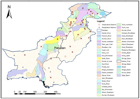
Figure A1.
Subbasin map of the study area and the precipitation and temperature stations used to compute the basin-averaged precipitation and temperature time series.
Figure A1.
Subbasin map of the study area and the precipitation and temperature stations used to compute the basin-averaged precipitation and temperature time series.
References
- IPCC, 2018: Global Warming of 1.5 °C. An IPCC Special Report on the Impacts of Global Warming of 1.5 °C above Pre-Industrial Levels and Related Global Greenhouse Gas Emission Pathways, in the Context of Strengthening the Global Response to the Threat of Climate Change, Sustainable Development, and Efforts to Eradicate Poverty. Available online: https://www.ipcc.ch/site/assets/uploads/sites/2/2019/06/SR15_Full_Report_Low_Res.pdf (accessed on 13 February 2022).
- Heikkila, E.J.; Huang, M. Adaptation to flooding in urban areas: An economic primer. Public Works Manag. Policy 2014, 19, 11–36. [Google Scholar] [CrossRef]
- Hassol, S.J.; Torok, S.; Lewis, S.; Luganda, P. Unnatural Disasters: Communicating Linkages Between Extreme Events and Climate Change; World Meteorological Organization (WMO): Geneva, Switzerland, 2017. [Google Scholar]
- Chu, J.T.; Xia, J.; Xu, C.-Y.; Singh, V.P. Statistical downscaling of daily mean temperature, pan evaporation and precipitation for climate change scenarios in Haihe River, China. Theor. Appl. Climatol. 2010, 99, 149–161. [Google Scholar] [CrossRef]
- Khattak, M.S.; Babel, M.S.; Sharif, M. Hydro-meteorological trends in the upper Indus River basin in Pakistan. Clim. Res. 2011, 46, 103–119. [Google Scholar] [CrossRef]
- Wang, J.; Ishidaira, H.; Xu, Z.X. Effects of climate change and human activities on inflow into the Hoabinh Reservoir in the Red River basin. Procedia Environ. Sci. 2012, 13, 1688–1698. [Google Scholar] [CrossRef] [Green Version]
- Pandey, V.P.; Shrestha, D.; Adhikari, M.; Shakya, S. Streamflow alterations, attributions, and implications in extended east Rapti watershed, central-southern Nepal. Sustainability 2020, 12, 3829. [Google Scholar] [CrossRef]
- Gemmer, M.; Becker, S.; Jiang, T. Detection and Visualisation of Climate Trends in China; Diskussionsbeiträge; Zentrum für Internationale Entwicklungs-und Umweltforschung: Kiel, Germany, 2003. [Google Scholar]
- Zhang, Q.; Jiang, T.; Gemmer, M.; Becker, S. Precipitation, temperature and runoff analysis from 1950 to 2002 in the Yangtze basin, China/Analyse des précipitations, températures et débits de 1950 à 2002 dans le bassin du Yangtze, en Chine. Hydrol. Sci. J. 2005, 50, 66–80. [Google Scholar] [CrossRef] [Green Version]
- Singh, P.; Kumar, V.; Thomas, T.; Arora, M. Basin-wide assessment of temperature trends in northwest and central India. Hydrol. Sci. J. 2008, 53, 421–433. [Google Scholar] [CrossRef]
- Huang, Y.; Cai, J.; Yin, H.; Cai, M. Correlation of precipitation to temperature variation in the Huanghe River (Yellow River) basin during 1957–2006. J. Hydrol. 2009, 372, 1–8. [Google Scholar] [CrossRef]
- Iqbal, M.S.; Dahri, Z.H.; Querner, E.P.; Khan, A. Impact of Climate Change on Flood Frequency and Intensity in the Kabul River Basin. Geosciences 2018, 5, 114. [Google Scholar] [CrossRef] [Green Version]
- Ahmad, I.; Tang, D.; Wang, T.; Wang, M.; Wagan, B. Precipitation trends over time using Mann-Kendall and spearman’s rho tests in swat river basin, Pakistan. Adv. Meteorol. 2015, 2015, 431860. [Google Scholar] [CrossRef] [Green Version]
- Shukla, P.R.; Skea, J.; Calvo Buendia, E.; Masson-Delmotte, V.; Pörtner, H.-O.; Roberts, D.C.; Zhai, P.; Slade, R.; Connors, S.; Van Diemen, R.; et al. IPCC, 2019: Climate Change and Land: An IPCC special report on climate change, desertification, land degradation, sustainable land management, food security, and greenhouse gas fluxes in terrestrial ecosystems. In Intergovernmental Panel on Climate Change (IPCC); United Nations: Geneva, Switzerland, 2019. [Google Scholar] [CrossRef]
- Zommers, Z.; van der Geest, K.; De Sherbinin, A.; Kienberger, S.; Roberts, E.; Harootunian, G.; Sitati, A.; James, R. Loss and Damage: The Role of Ecosystem Services; United Nations Environment Programme: Nairobi, Kenya, 2016; p. 84. [Google Scholar]
- The Institute for Economics and Peace. Global Peace Index 2017—Measuring Peace in a Complex World; The Institute for Economics and Peace: Sydney, Australia, 2018; Volume 1, pp. 1–140. [Google Scholar]
- Eckstein, D.; Künzel, V.; Schäfer, L.; Winges, M. Global Climate Risk Index 2020; Germanwatch: Bonn, Germany, 2019; Volume 1, pp. 1–44. [Google Scholar]
- Rehman, A.; Jingdong, L.; Shahzad, B.; Chandio, A.A.; Hussain, I.; Nabi, G.; Iqbal, M.S. Economic perspectives of major field crops of Pakistan: An empirical study. Pac. Sci. Rev. B Humanit. Soc. Sci. 2015, 1, 145–158. [Google Scholar] [CrossRef] [Green Version]
- Ramachandran, V.; Ramalakshmi, R.; Kavin, B.P.; Hussain, I.; Almaliki, A.H.; Almaliki, A.A.; Elnaggar, A.Y.; Hussein, E.E. Exploiting IoT and Its Enabled Technologies for Irrigation Needs in Agriculture. Water 2022, 14, 719. [Google Scholar] [CrossRef]
- Talchabhadel, R.; Aryal, A.; Kawaike, K.; Yamanoi, K.; Nakagawa, H.; Bhatta, B.; Karki, S.; Thapa, B.R. Evaluation of precipitation elasticity using precipitation data from ground and satellite-based estimates and watershed modeling in Western Nepal. J. Hydrol. Reg. Stud. 2021, 33, 100768. [Google Scholar] [CrossRef]
- Vano, J.A.; Das, T.; Lettenmaier, D.P. Hydrologic sensitivities of Colorado River runoff to changes in precipitation and temperature. J. Hydrometeorol. 2012, 13, 932–949. [Google Scholar] [CrossRef] [Green Version]
- Zuo, D.; Xu, Z.; Wu, W.; Zhao, J.; Zhao, F. Identification of streamflow response to climate change and human activities in the wei river Basin, China. Water Resour. Manag. 2014, 28, 833–851. [Google Scholar] [CrossRef]
- Sun, S.; Chen, H.; Ju, W.; Song, J.; Zhang, H.; Sun, J.; Fang, Y. Effects of climate change on annual streamflow using climate elasticity in Poyang Lake Basin, China. Theor. Appl. Climatol. 2013, 112, 169–183. [Google Scholar] [CrossRef]
- Junior, D.S.R.; Cerqueira, C.M.; Vieira, R.F.; Martins, E.S. Budyko’s Framework and Climate Elasticity Concept in the Estimation of Climate Change Impacts on the Long-Term Mean Annual Streamflow. World Environ. Water Resour. Congr. 2013, 2013, 1110–1120. [Google Scholar] [CrossRef]
- Frederick, K.D.; Major, D.C. Climate Change and Water Resources. Clim. Chang. 1997, 37, 7–23. [Google Scholar] [CrossRef]
- Nash, L.L.; Gleick, P.H. Sensitivity of streamflow in the Colorado basin to climatic changes. J. Hydrol. 1991, 125, 221–241. [Google Scholar] [CrossRef]
- Jeton, A.E.; Dettinger, M.D.; Smith, J.L. Potential effects of climate change on streamflow, eastern and western slopes of the Sierra Nevada, California and Nevada. Water Resour. Investig. Rep. 1996, 95, 4260. [Google Scholar]
- Sankarasubramanian, A.; Vogel, R.M.; Limbrunner, J.F. Climate elasticity of streamflow in the United States. Water Resour. Res. 2001, 37, 1771–1781. [Google Scholar] [CrossRef]
- Jones, R.N.; Chiew, F.H.S.; Boughton, W.C.; Zhang, L. Estimating the sensitivity of mean annual runoff to climate change using selected hydrological models. Adv. Water Resour. 2006, 29, 1419–1429. [Google Scholar] [CrossRef] [Green Version]
- Karki, M.B.; Shrestha, A.B.; Winiger, M. Enhancing Knowledge Management and Adaptation Capacity for Integrated Management of Water Resources in the Indus River Basin. Mt. Res. Dev. 2011, 31, 242–251. [Google Scholar] [CrossRef]
- Khan, A.; Richards, K.; Mcrobie, F.A.; Booij, M.J. Impact of warming climate on the monsoon and water resources of a western Himalayan watershed in the Upper Indus Basin. In Proceedings of the EGU General Assembly, Vienna, Austria, 12–17 April 2015; p. 7798. [Google Scholar]
- Ludwig, F.; Hussain, Z.; Ludwig, F.; Moors, E.; Ahmad, B.; Khan, A.; Kabat, P. An appraisal of precipitation distribution in the high-altitude catchments of the Indus basin. Sci. Total Environ. 2016, 548, 289–306. [Google Scholar] [CrossRef] [Green Version]
- Mahmood, R.; Jia, S. Assessment of impacts of climate change on the water resources of the transboundary Jhelum River Basin of Pakistan and India. Water 2016, 8, 246. [Google Scholar] [CrossRef] [Green Version]
- Adnan, S.; Ullah, K.; Khan, A.H.; Shouting, G.A.O. Meteorological impacts on evapotranspiration in different climatic zones of Pakistan. J. Arid. Land 2017, 9, 938–952. [Google Scholar] [CrossRef] [Green Version]
- Zaman, S.; Hussain, I.; Singh, D. Fast Computation of Integrals with Fourier-Type Oscillator Involving Stationary Point. Mathematics 2019, 7, 1160. [Google Scholar] [CrossRef] [Green Version]
- Kidd, C.; Becker, A.; Huffman, G.J.; Muller, C.L.; Joe, P.; Skofronick-Jackson, G.; Kirschbaum, D.B. So, how much of the Earth’s surface is covered by rain gauges? Bull. Am. Meteorol. Soc. 2017, 98, 69–78. [Google Scholar] [CrossRef]
- Akhtar, M.; Ahmad, N.; Booij, M.J. The impact of climate change on the water resources of Hindukush-Karakorum-Himalaya region under different glacier coverage scenarios. J. Hydrol. 2008, 355, 148–163. [Google Scholar] [CrossRef]
- Sankarasubramanian, A.; Vogel, R.M. Hydroclimatology of the continental United States. Geophys. Res. Lett. 2003, 30, 1363. [Google Scholar] [CrossRef]
- Tsai, Y. The multivariate climatic and anthropogenic elasticity of streamflow in the Eastern United States. J. Hydrol. Reg. Stud. 2017, 9, 199–215. [Google Scholar] [CrossRef]
- Yu, J.; Fu, G.; Cai, W.; Cowan, T. Impacts of precipitation and temperature changes on annual streamflow in the Murray-Darling Basin. Water Int. 2010, 35, 313–323. [Google Scholar] [CrossRef]
- Fu, G.; Chiew, F.H.S.; Charles, S.P.; Mpelasoka, F. Assessing precipitation elasticity of streamflow based on the strength of the precipitation-streamflow relationship. In Proceedings of the 19th International Congress on Modelling and Simulation, MODSIM 2011, Perth, Auatralia, 12–16 December 2011; pp. 3567–3572. [Google Scholar]
- Yang, H.; Yang, D. Derivation of climate elasticity of runoff to assess the effects of climate change on annual runoff. Water Resour. Res. 2011, 47, W07526. [Google Scholar] [CrossRef]
- Li, F.; Zhang, G.; Xu, Y.J. Separating the impacts of climate variation and human activities on runoff in the Songhua River Basin, Northeast China. Water 2014, 6, 3320–3338. [Google Scholar] [CrossRef] [Green Version]
- Zhou, X.; Zhang, Y.; Yang, Y. Comparison of Two Approaches for Estimating Precipitation Elasticity of Streamflow in China’s Main River Basins. Adv. Meteorol. 2015, 2015, 924572. [Google Scholar] [CrossRef]
- Andréassian, V.; Coron, L.; Lerat, J.; Le Moine, N. Climate elasticity of streamflow revisited—An elasticity index based on long-term hydrometeorological records. Hydrol. Earth Syst. Sci. 2016, 20, 4503–4524. [Google Scholar] [CrossRef] [Green Version]
- Vogel, R.; Wilson, I.; Drainage, C.D. Regional Regression Models of Annual Streamflow for the United States. J. Irrig. Drain. Eng. 1999, 125, 148–157. Available online: https://ascelibrary.org/doi/abs/10.1061/(ASCE)0733-9437(1999)125:3(148) (accessed on 3 March 2019). [CrossRef]
- Ma, H.; Yang, D.; Tan, S.K.; Gao, B.; Hu, Q. Impact of climate variability and human activity on streamflow decrease in the Miyun Reservoir catchment. J. Hydrol. 2010, 389, 317–324. [Google Scholar] [CrossRef]
- Fu, G.; Charles, S.P.; Chiew, F.H.S. A two-parameter climate elasticity of streamflow index to assess climate change effects on annual streamflow. Water Resour. Res. 2007, 43, 1–12. [Google Scholar] [CrossRef]
- Hussain, I.; Ullah, M.; Ullah, I.; Bibi, A.; Naeem, M.; Singh, M.; Singh, D. Optimizing Energy Consumption in the Home Energy Management System via a Bio-Inspired Dragonfly Algorithm and the Genetic Algorithm. Electronics 2020, 9, 406. [Google Scholar] [CrossRef]
- Bartsotas, N.S.; Anagnostou, E.N.; Nikolopoulos, E.I.; Kallos, G. Investigating Satellite Precipitation Uncertainty Over Complex Terrain. J. Geophys. Res. Atmos. 2018, 123, 5346–5359. [Google Scholar] [CrossRef]
- Derin, Y.; Yilmaz, K.K. Evaluation of multiple satellite-based precipitation products over complex topography. J. Hydrometeorol. 2014, 15, 1498–1516. [Google Scholar] [CrossRef] [Green Version]
- Mei, Y.; Nikolopoulos, E.I.; Anagnostou, E.N.; Borga, M. Evaluating satellite precipitation error propagation in runoffsimulations of mountainous basins. J. Hydrometeorol. 2016, 17, 1407–1423. [Google Scholar] [CrossRef]
- Hussain, I.; Samara, G.; Ullah, I.; Khan, N. Encryption for End-User Privacy: A Cyber-Secure Smart Energy Management System. In Proceedings of the 2021 22nd International Arab Conference on Information Technology (ACIT), Muscat, Oman, 21–23 December 2021; pp. 1–6. [Google Scholar] [CrossRef]
- Liu, R.F.; Li, P.Y.; Chen, X.T.; Hou, J.Z. Analysis of a flood rainstorm caused by MCC in Shaanxi. J. Chengdu Univ. Inf. Technol. 2012, 27, 306–313. [Google Scholar]
- Ullah, I.; Hussain, I.; Rehman, K.; Wroblewski, P.; Lewicki, W.; Kavin, B.P. Exploiting the Moth–Flame Optimization Algorithm for Optimal Load Management of the University Campus: A Viable Approach in the Academia Sector. Energies 2022, 15, 3741. [Google Scholar] [CrossRef]
- Liu, Z.; Zhang, X.; Fang, R. Multi-scale linkages of winter drought variability to ENSO and the Arctic Oscillation: A case study in Shaanxi, North China. Atmos. Res. 2018, 200, 117–125. [Google Scholar] [CrossRef]
- Meng, Q.; Bai, H.; Zhao, T.; Guo, S.; Qi, G. Topographic characteristic of climate change in the Qinling mountains. China Mt. Res. 2020, 38, 180–189. [Google Scholar]
- Zhu, L.; Meng, Z.; Zhang, F.; Markowski, P.M. The influence of sea-and land-breeze circulations on the diurnal variability in precipitation over a tropical island. Atmos. Chem. Phys. 2017, 17, 13213–13232. [Google Scholar] [CrossRef] [Green Version]
- Ullah, W.; Hussain, I.; Shehzadi, I.; Rahman, Z.; Uthansakul, P. Tracking a Decentralized Linear Trajectory in an Intermittent Observation Environment. Sensors 2020, 20, 2127. [Google Scholar] [CrossRef] [PubMed] [Green Version]
- Viale, M.; Garreaud, R. Orographic effects of the subtropical and extratropical Andes on upwind precipitating clouds. J. Geophys. Res. Atmos. 2015, 120, 4962–4974. [Google Scholar] [CrossRef]
- Kanda, N.; Negi, H.S.; Rishi, M.S.; Kumar, A. Performance of various gridded temperature and precipitation datasets over northwest himalayan region. Environ. Res. Commun. 2020, 2, 2000–2008. [Google Scholar] [CrossRef]
- Han, S.; Shi, C.; Sun, S.; Gu, J.; Xu, B.; Liao, Z.; Zhang, Y.; Xu, Y. Development and Evaluation of a Real-Time Hourly One-Kilometre Gridded Multisource Fusion Air Temperature Dataset in China Based on Remote Sensing DEM. Remote Sens. 2022, 14, 2480. [Google Scholar] [CrossRef]
- Prabakaran, S.; Ramar, R.; Hussain, I.; Kavin, B.P.; Alshamrani, S.S.; AlGhamdi, A.S.; Alshehri, A. Predicting Attack Pattern via Machine Learning by Exploiting Stateful Firewall as Virtual Network Function in an SDN Network. Sensors 2022, 22, 709. [Google Scholar] [CrossRef]
- Sarfaraz, S.; Hasan Arsalan, M.; Fatima, H. Regionalizing the Climate of Pakistan Using Köppen Classification System. Pakistan Geogr. Rev. 2014, 69, 111–132. [Google Scholar]
- Wolf, A.T.; Natharius, J.A.; Danielson, J.J.; Ward, B.S.; Pender, J.K. International river basins of the world. Int. J. Water Resour. Dev. 1999, 15, 387–427. [Google Scholar] [CrossRef]
- FAO. Report on Indus River Basin. 2011, pp. 1–14. Available online: http://www.fao.org/nr/water/aquastat/basins/indus/index.stm (accessed on 13 February 2022).
- Shaheen, F.; Shah, F. Climate Change, Economic Growth, and Cooperative Management of Indus River Basin. 2017. Available online: https://ageconsearch.umn.edu/record/258350/files/Abstracts_17_05_24_16_49_13_59__137_99_85_24_0.pdf (accessed on 1 March 2019).
- Ojeh, E. Hydrology of the Indus Basin (Pakistan). 2006. Available online: https://waterinfo.net.pk/sites/default/files/knowledge/HydrologyoftheIndusBasin.pdf (accessed on 2 March 2019).
- International Monetary Fund Issues in Managing Water Challenges and Policy Instruments: Regional Perspectives and Case Studies. 2015. Available online: https://www.imf.org/external/pubs/ft/sdn/2015/sdn1511tn.pdf (accessed on 29 April 2022).
- Khan, M.A.; Khan, J.A.; Ali, Z.; Ahmad, I.; Ahmad, M.N. The challenge of climate change and policy response in Pakistan. Environ. Earth Sci. 2016, 75, 412. [Google Scholar] [CrossRef]
- USGS. Science for a Changing World. Available online: https://earthexplorer.usgs.gov (accessed on 31 December 2021).
- Chiew, F.H.S.; Peel, M.C.; McMahon, T.A.; Siriwardena, L.W. Precipitation elasticity of streamflow in catchments across the world. PPT Present. 2006, 308, 256–262. [Google Scholar]
- Pakistan Meteorological Department (PMD). Available online: https://pmd.gov.pk (accessed on 31 December 2021).
- Water and Power Development Authority (WAPDA). Available online: https://wapda.gov.pk (accessed on 31 December 2021).
- Global Runoff Data Center (GRDC). Available online: https://bafg.de/GRDC/EN/Home/homepage_node.html (accessed on 31 December 2021).
- Li, E.; Mu, X.; Zhao, G.; Gao, P.; Shao, H. Variation of runoff and precipitation in the hekou-longmen region of the yellow river based on elasticity analysis. Sci. World J. 2014, 2014, 929858. [Google Scholar] [CrossRef]
- Allaire, M.C.; Vogel, R.M.; Kroll, C.N. The hydromorphology of an urbanizing watershed using multivariate elasticity. Adv. Water Resour. 2015, 86, 147–154. [Google Scholar] [CrossRef]
- Shah, L.A.; Khan, A.U.; Khan, F.A.; Khan, Z.; Rauf, A.U.; Rahman, S.U.; Iqbal, M.J.; Ahmad, I.; Abbas, A. Statistical significance assessment of streamflow elasticity of major rivers. Civ. Eng. J. 2021, 7, 893–905. [Google Scholar] [CrossRef]
- Saifullah, M.; Adnan, M.; Zaman, M.; Wałęga, A.; Liu, S.; Khan, M.I.; Gagnon, A.S.; Muhammad, S. Hydrological response of the kunhar river basin in pakistan to climate change and anthropogenic impacts on runoff characteristics. Water 2021, 13, 3163. [Google Scholar] [CrossRef]
- Hanif, M.; Hayyat, A.; Adnan, S. Latitudinal precipitation characteristics and trends in Pakistan. J. Hydrol. 2013, 492, 266–272. [Google Scholar] [CrossRef]
- Hussain, I.; Ullah, I.; Ali, W.; Muhammad, G.; Ali, Z. Exploiting lion optimization algorithm for sustainable energy management system in industrial applications. Sustain. Energy Technol. Assess. 2022, 52, 102237. [Google Scholar] [CrossRef]
- Chiew, F.; Potter, N.; Vaze, J.; Petheram, C.; Zhang, L.; Teng, J.; Post, D.A. Observed hydrologic non-stationarity in far south-eastern Australia: Implications for modelling and prediction. Stoch. Environ. Res. Risk Assess. 2014, 28, 3–15. Available online: https://link.springer.com/article/10.1007/s00477-013-0755-5 (accessed on 26 May 2019). [CrossRef]
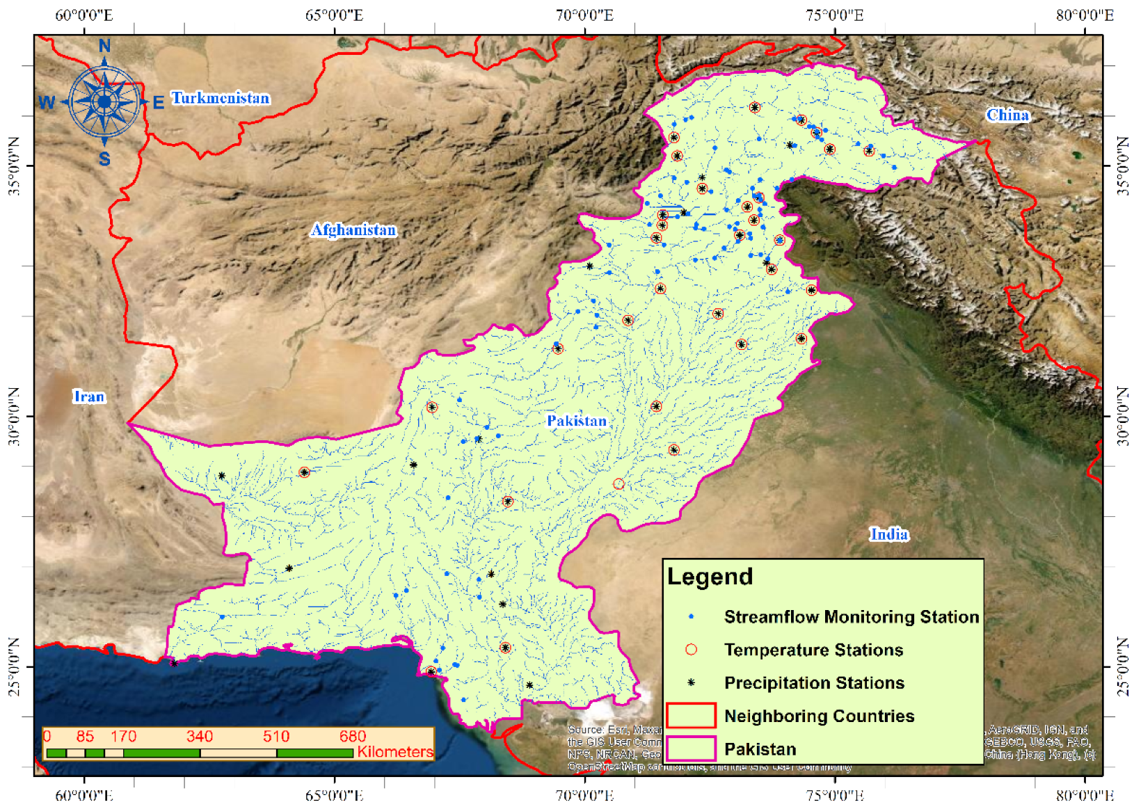

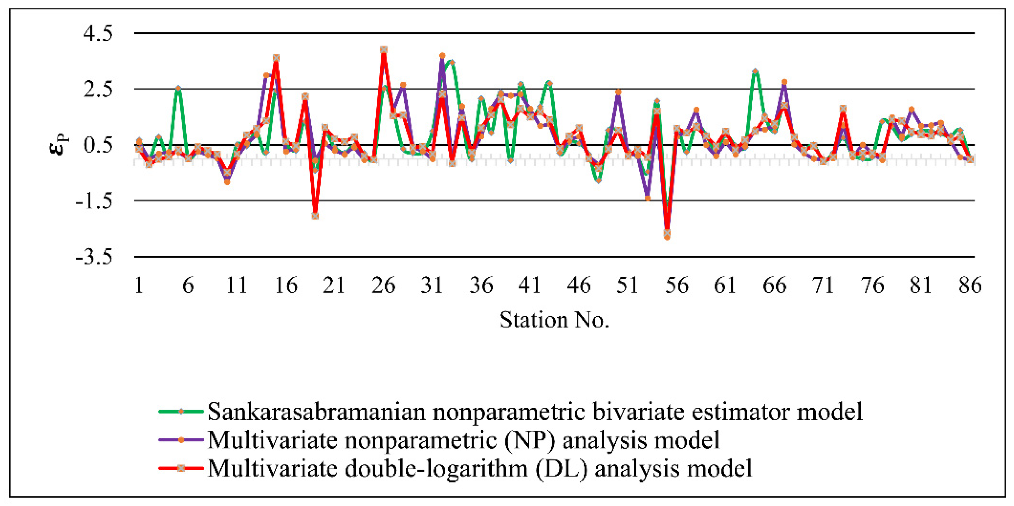
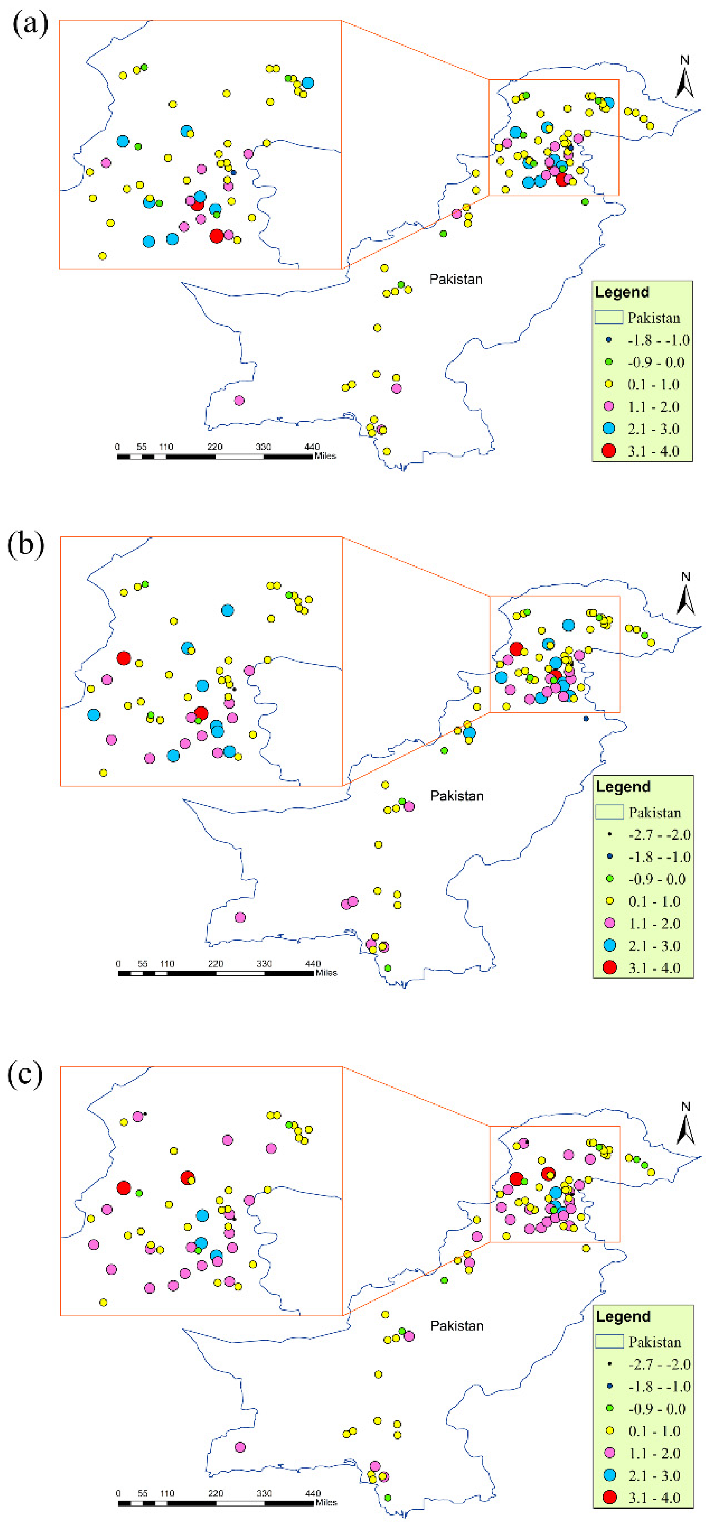
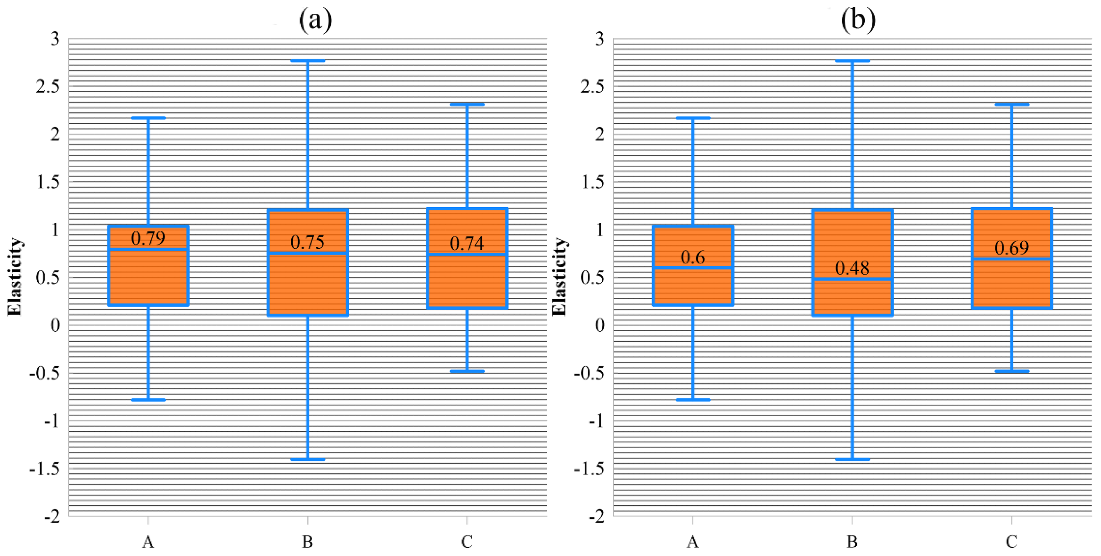

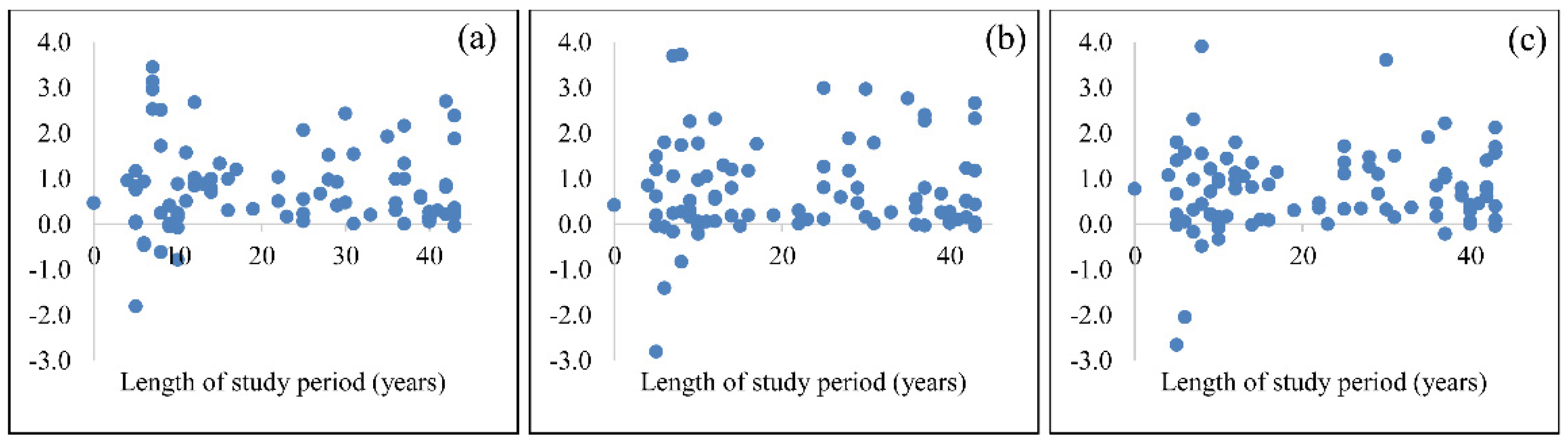
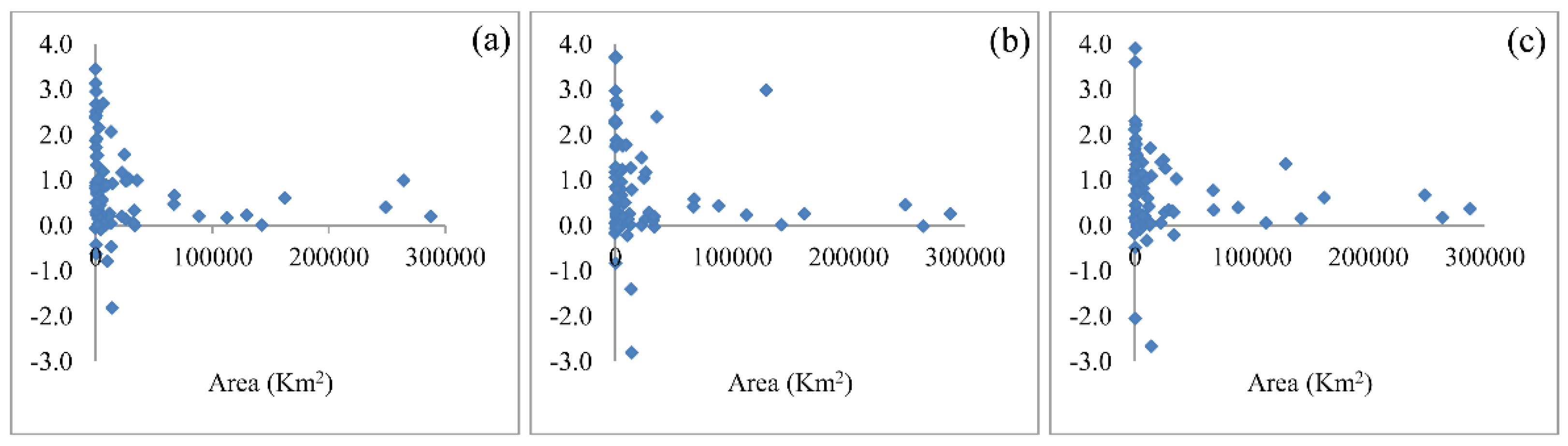
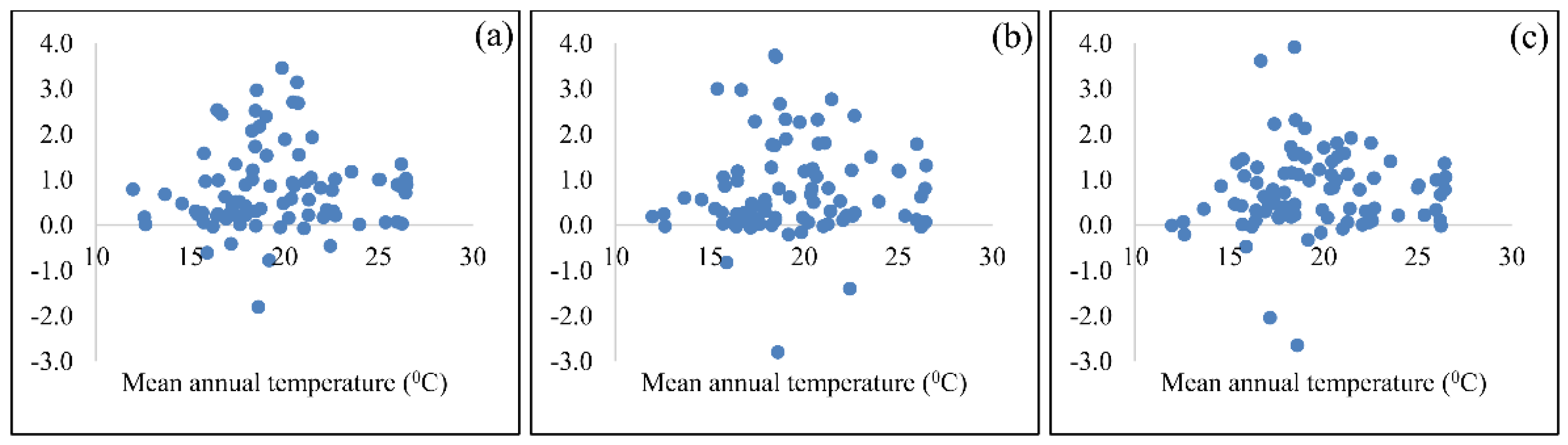
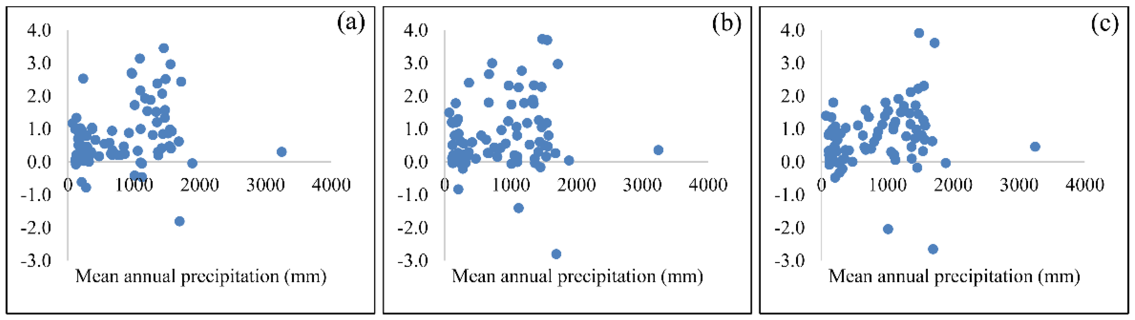
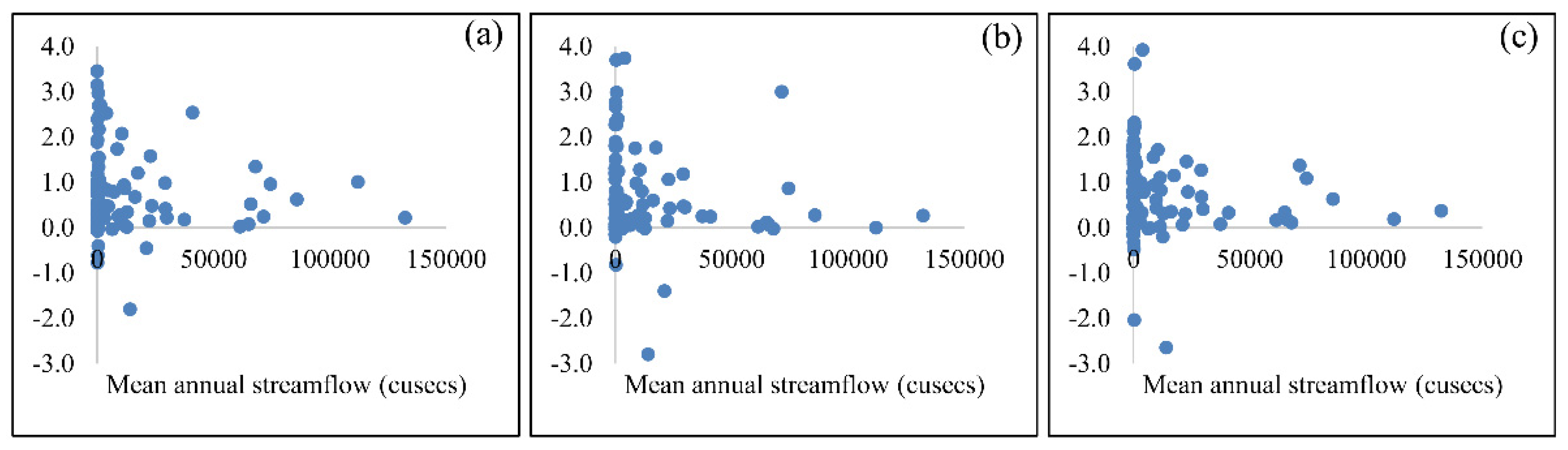

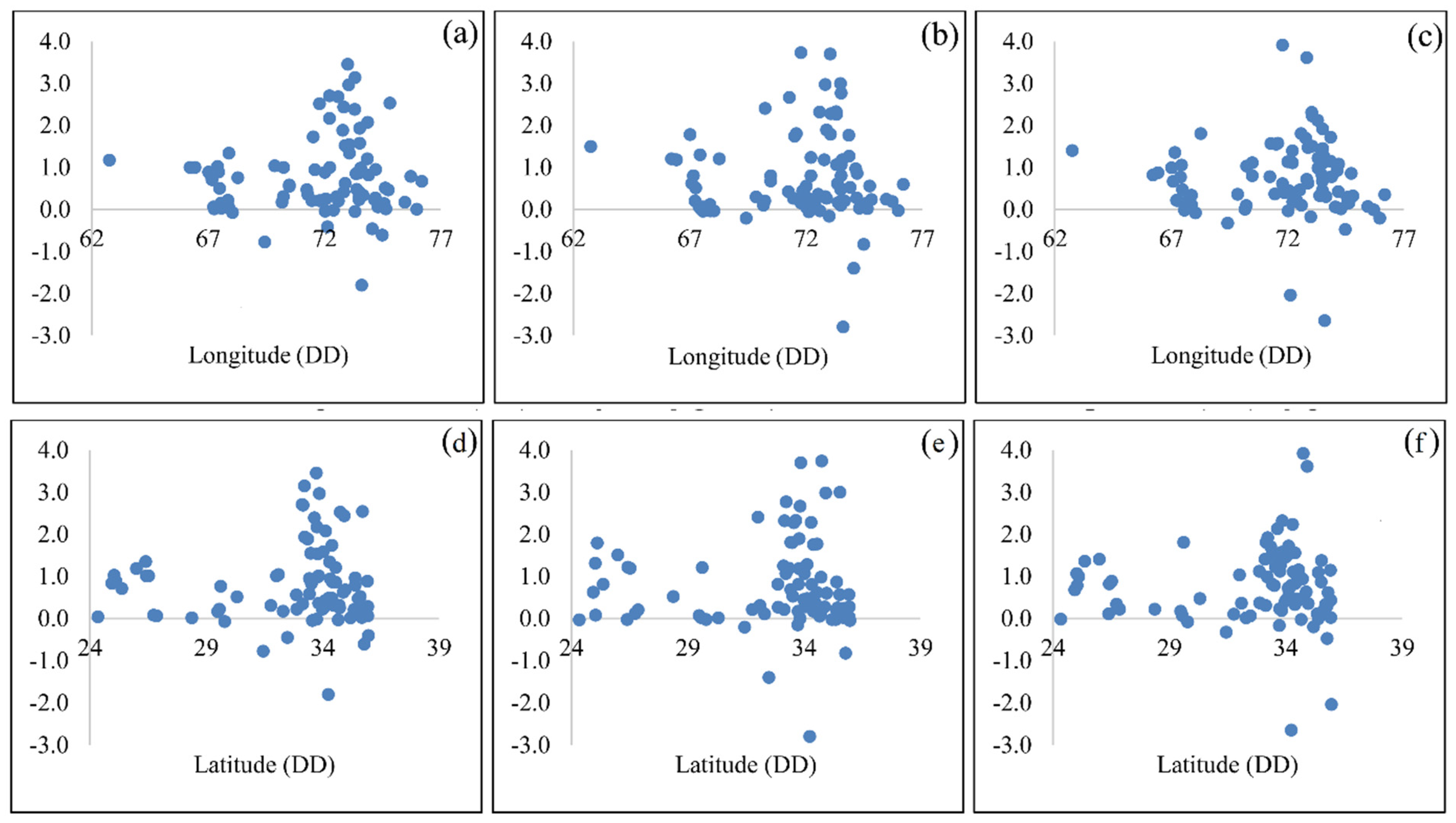


Publisher’s Note: MDPI stays neutral with regard to jurisdictional claims in published maps and institutional affiliations. |
© 2022 by the authors. Licensee MDPI, Basel, Switzerland. This article is an open access article distributed under the terms and conditions of the Creative Commons Attribution (CC BY) license (https://creativecommons.org/licenses/by/4.0/).