A Comparative Study of Breaking Wave Loads on Cylindrical and Conical Substructures

Abstract

In the present paper, a comparative study of different cylindrical and conical substructures was performed under breaking wave loading with the open-source Computational Fluid Dynamics (CFD) package OpenFoam capable of the development of a numerical wave tank (NWT) with the use of Reynolds-Averaged Navier–Stokes (RANS) equations, the k-ω Shear Stress Transport (k-ω SST) turbulence model, and the volume of fluid (VOF) method. The validity of the NWT was verified with relevant experimental data. Then, through the application of the present numerical model, the distributions of dynamic pressure and velocity in the x-direction around the circumference of different cylindrical and conical substructures were examined. The results showed that the velocity and dynamic pressure distribution did not change significantly with the increase in the substructure’s diameter near the wave breaking height, although the incident wave conditions were similar. Another important aspect of the study was whether the hydrodynamic loading or the dynamic pressure distribution of a conical substructure would improve or deteriorate under the influence of breaking wave loading compared to a cylindrical one. It was concluded that the primary wave load in a conical substructure increased by 62.57% compared to the numerical results of a cylindrical substructure. In addition, the secondary load’s magnitude in the conical substructure was 3.39 times higher and the primary-to-secondary load ratio was double compared to a cylindrical substructure. These findings demonstrate that the conical substructure’s performance will deteriorate under breaking wave loading compared to a cylindrical one, and it is not recommended to use this type of substructure.

1. Introduction

Marine renewable energy was generating considerable interest on a worldwide scale due to the effects of climate change and energy demand leading to offshore wind turbine substructures (OWTs). Various substructures can be chosen depending on the varying water depths and installation capabilities. Bottom-fixed substructures including monopile, jacket, gravity base, and tripod can be installed in shallow and intermediate water depths because they are relatively simple to construct, less costly, and easier to install near the coast [1]. According to [2], up-to-date monopiles remain the most installed foundation with 4258 units representing 81% in Europe.

To begin with, as the wave develops in shallow and intermediate depths, the wave’s amplitude approaches a crucial point at which it becomes unstable and breaks. The wave energy extracted from the wave-breaking process is converted into turbulent kinetic energy. Due to the nonlinear breaking loads, extremely transient hydrodynamic loads are presented near the substructure. As expected, OWT capacities increase every year. It is noteworthy that since 2014, the turbine capability has seen an increase of 16% every year on average. Moreover, the offshore wind farms’ average water depth slightly increased from 30 m in 2018 to 33 m in 2019.

Nevertheless, as the OWTs become larger and are installed in deeper water, the structural integrity is challenged significantly as wave loads increasingly conflict with the substructure dynamics. A vital factor influencing the hydrodynamic performance is the diameter of an OWT’s monopile. As the substructure diameter becomes larger, the nonlinear wave structure interaction is especially noticeable. Accordingly, for the design of OWT substructures in shallow or intermediate depths, the monopile diameter and the wave impact loads are critical factors affecting the structural integrity and survivability of any marine (coastal and offshore) structure systems.

Several initial studies on the wave-breaking phenomenon were limited to experiments in an attempt to find an analytical solution, due to the complexity and the high nonlinearity of this phenomenon. Wienke & Oumeraci [3] studied the breaking wave impact properties on a slender cylinder. Their findings showed that the breaking wave impact force was influenced by several parameters, such as the breaking type, the breaking depth, and the breaker position length from the cylinder. Wienke et al. [4] examined the breaking wave impact on a vertical monopile using a large-scale experimental setup. The experiments demonstrated that the quasi-static force calculated by the Morison equation and the slamming force considering the impact’s period were equal to the total breaking wave force. Furthermore, the Fast Fourier Transform (FFT) low-pass filter and the Empirical Mode Decomposition (EMD) were applied by K Irschik et al. [5] to decompose the experimental data of breaking wave forces into two components, the quasi-static loading and the slamming force. Their investigation highlighted that the quasi-static force was overestimated with the calculation methods in the area of the maximum impact.

A possible solution to these challenges could be a well-validated numerical model based on Computational Fluid Dynamics (CFD). This model will be capable of solving the Navier–Stokes equations and simulate breaking wave interaction with structures. The modelling of the wave breaking phenomenon over slopes with different geometries was investigated by many researchers. Liu et al. [6] applied the k-ω Shear Stress Transport (SST) turbulence model and the Volume of Fluid (VOF) method to examine the characteristics of higher-harmonic breaking wave forces and secondary load cycles on a single vertical circular cylinder at various Froude numbers by modifying the diameter and incident wave conditions. They observed that the secondary load cycles occurred at a Froude number exceeding 0.4 for non-breaking wave cases, and the magnitudes of the secondary load cycles ranged between 8.1% and 12.6% of the peak-to-peak wave force. It can be argued that the Froude number decreased at 0.35, and the magnitudes of the secondary load cycles decreased by between 2.4% and 7.6% of the peak-to-peak wave force for the breaking wave case. Adding to this, the secondary load cycle duration was shorter than 24.2% of the wave period T for all the simulated cases. Qu et al. [7] employed the k-ω SST turbulence model and the VOF method to study the breaking wave loading on standing circular cylinders with several transverse inclined angles. Their research concluded that when the cylinder’s transverse inclined angle was 45°, the free surface elevations in front of the cylinder and the normalized high-order wave force had the smallest value. Another finding suggested that when the cylinder was placed with transverse inclined angles of 30° and 45, the secondary load creating the higher harmonic ringing motion of structures did not occur. Jose et al. [8] used the k–ω SST turbulence model to generate the breaking wave forces on a vertical monopile with two separate solvers based on the finite volume method (OpenFoam) and finite difference method (2PM3D). The two solvers were capable of simulating breaking waves since the numerical results showed good agreement with the experimental data. Liu et al. [9] studied the breaking waves and steep waves past a vertical cylinder at varying Keulegan–Carpenter (KC) numbers using the k-ω SST turbulence model and the VOF method. They observed that when the KC number increased, the horizontal wave force’s peak value increased on the structure. In addition, when the incident wave height increased, the maximum dynamic pressure increased, but it did not change significantly with varying diameters. Moreover, the highest dynamic pressures occurred at the cylinder’s rear point due to the interaction of the return flow with the cylinder. However, the secondary load cycle’s behaviour was more sensitive to the cylinder’s different diameter than the incident wave height. Chella et al. [10] examined the breaking wave impact on a vertical cylinder with the CFD software REEF3D implementing the k-ω turbulence model and the level set method (LSM). They concluded that when the wave steepness increased, the impact pressure rise time increased. Further, the vertical velocity first reached its maximum value for a specific impact condition and wave steepness, followed by the horizontal velocity and the pressure. Moreover, when the wave broke ahead of the cylinder and impacted a moderate overturning wave crest for several wave steepness values, the largest breaking wave force occurred. Kamath et al. [11] utilized the k–ω turbulence model and the level set method and analysed the wave structure interactions among a single monopile at varying breaker locations with plunging breaking conditions. They found that the wave breaking position was correlated with the breaking wave forces on the substructure. When the overturning wave crest passed the substructure, the largest force was observed, and when the wave broke behind the substructure the smallest force was observed.

In the present study, numerical simulations of different cylindrical and conical substructures were performed in a developed Numerical Wave Tank (NWT) applying the Reynolds Averaged Navier Stokes (RANS) equations with the use of the k-ω SST turbulence model and the VOF method in OpenFoam. The present numerical model was verified with available experimental data. Afterwards, the velocity and dynamic pressure distribution around the circumference of different conical and cylindrical substructures were investigated. This comparison showed that the distribution of velocity and dynamic pressure did not change significantly near the wave breaking height with the change in the substructure type and the increase in the diameter, although the incident wave conditions were the same. Furthermore, this paper investigated whether the hydrodynamic loading or the distribution of dynamic pressure of a different substructure with a conical shape would improve or deteriorate under the influence of breaking wave loads compared to a cylindrical substructure. The findings of this research indicate that the primary wave load increased by 62.57% compared to the numerical results of a cylindrical substructure. Further, the magnitude of the secondary load in the conical substructure was 3.39 times higher and the primary-to-secondary wave load ratio was double compared to the cylindrical substructure. Based on the simulations performed and the observations made, it is not recommended to use a conical substructure in place of a cylindrical one.

2. Numerical Model

2.1. Governing Equations

In the present numerical model, the simulations were performed with the open-source CFD package OpenFoam. The solver used for all the simulations was InterFoam, suitable for incompressible, isothermal fluids using the Finite Volume Method (FVM) discretization and the VOF method for the interface capturing.

RANS equations were applied, decomposing all the terms into a mean and a fluctuating component in order to describe the turbulent effects. From the decomposition of the equations, the Reynolds stress tensor $\mathsf{\rho }\overline{{{\mathbf{u}}_{\mathrm{i}}}^{\prime }{{\mathbf{u}}_{\mathrm{j}}}^{\prime }}$ derives were obtained, representing the turbulent fluctuations. In order to close the system of equations, the Reynolds stress tensor was modelled as a function of the mean flow excluding the velocity’s fluctuating component, including the mean velocity and pressure. A well-known approach uses the Boussinesq hypothesis to associate the Reynolds stresses with the mean velocity gradient to close the system of equations as follows:

$$\overline{{{\mathbf{u}}_{\mathrm{i}}}^{\prime }{{\mathbf{u}}_{\mathrm{j}}}^{\prime }}=-{\mathsf{\mu }}_{\mathsf{\tau }}\left(\nabla \mathbf{u}+\nabla {\mathbf{u}}^{\mathrm{T}}\right)+\frac{2}{3}{\mathrm{k}\mathsf{\delta }}_{\mathrm{ij}}$$

(1)

where δ_ij is the Kronecker delta function, μ_τ is the turbulent eddy viscosity, and k is the turbulent kinetic energy.

The final form of the mass conservation equation and the momentum conservation equation applying the RANS equations are shown below.

$$\nabla ·\mathbf{u}=0$$

(2)

$$\mathsf{\rho }\frac{\partial \mathbf{u}}{\partial \mathrm{t}}+\mathsf{\rho }\nabla ·(\mathbf{u}{\mathbf{u}}^{\mathrm{T}})-\nabla ·({\mathsf{\mu }}_{\mathrm{eff}}\nabla \mathbf{u})=-\nabla {\mathrm{P}}_{\mathrm{rgh}}+{\mathbf{F}}_{\mathsf{\sigma }}$$

(3)

In Equation (3), the first term is the local time variation of momentum and the second term is the transport of momentum due to the velocity field. The stress tensor’s gradient for incompressible flow is the third term, where μ_eff is the efficient dynamic viscosity. The pressure gradient acting on the fluid is the first term on the right-hand side, where P_rgh is the dynamic pressure. InterFoam solver uses P_rgh instead of the pressure relative to the local hydrostatic pressure ρg_ix_i, where P_rgh = P − ρg_ix_i. The setting of the boundary conditions will be complicated because the pressure relative to the hydrostatic pressure is a function of the cell position. In contrast, using P_rgh in the momentum equation, uniform boundary conditions will be achieved without considering the locations of different fluids. The last term of Equation (3) is the surface tension force F_σ. The surface tension can be estimated by using the Continuum Surface Force (CSF) model of [12]. According to Heller [13], the surface tension force is negligible for large-scale models and most prototypes in hydraulic engineering. Furthermore, the surface tension force contribution compared to inertial force is smaller than 1% when the deep-water wave period is longer than 0.35 s and the deep-water wave height is greater than 0.02 m [14]. Therefore, the surface tension force is considered negligible and was set to zero in the present study.

2.2. Free Surface Modelling

The position and the development of the free surface between the water and air phase of the computational domain must be computed as part of the solution. The free surface is modelled adopting the VOF method introduced by Hirt & Nickols [15] in OpenFoam. A supplementary equation is needed to define the free surface movement. Therefore, only an indicator phase function α is required. The indicator phase function is defined as the amount of water per unit of volume in each computational domain cell. This indicates that if α = 1, then the cell is full of water; if α = 0, then the cell is full of air and in between it pertains to the interface.

$$\mathsf{\alpha }(\mathrm{x},\mathrm{t})=\{\begin{array}{ll}1,& \mathrm{water}\\ 0,& \mathrm{air}\\ 0<{\mathsf{\alpha }}_{\mathrm{s}}<1,& \mathrm{interface}\end{array}$$

(4)

The fluid properties in every cell can be calculated by weighting them by the VOF function. For example, the density of the cell and dynamic viscosity are computed as follows:

$$\mathsf{\rho }=\mathsf{\alpha }{\mathsf{\rho }}_{\mathrm{water}}+(1-\mathsf{\alpha }){\mathsf{\rho }}_{\mathrm{air}}$$

(5)

$$\mathsf{\mu }=\mathsf{\alpha }{\mathsf{\mu }}_{\mathrm{water}}+(1-\mathsf{\alpha }){\mathsf{\mu }}_{\mathrm{air}}$$

(6)

The transport equation that defines the fluid elevation is a classic advection equation, as displayed below.

$$\frac{\partial \mathsf{\alpha }}{\partial \mathrm{t}}+\nabla ·(\mathbf{u}\mathsf{\alpha })=0$$

(7)

However, to obtain physical results, some limitations need to be employed. The phase indicator α needs to be conservative and bounded between 0 and 1. The equation boundedness is performed using a solver called MULES (Multidimensional Universal Limiter for Explicit Solution). It uses a limiter factor on the discretized divergence term’s fluxes to guarantee a final value between 0 and 1. For additional reference concerning the governing equations, see [16]. Another limitation is that the interface must be kept small enough because the free surface in actual liquids is a sharp discontinuity. Accordingly, a careful choice must be made for the scheme used for the α field’s advection. For the advection equation solution, a common finite-volume approach would lead to the smearing of the interface. An artificial compression term $\partial {\mathbf{u}}_{\mathrm{r}}\mathsf{\alpha }(1-\mathsf{\alpha })$ is included in areas with phase indicator fractions varying from 0 and 1; this is reduced as shown below:

$$\frac{\partial \mathsf{\alpha }}{\partial \mathrm{t}}+\nabla ·(\mathbf{u}\mathsf{\alpha })+\nabla ·[\mathsf{\alpha }(1-\mathsf{\alpha }){\mathbf{u}}_{\mathrm{r}}]=0$$

(8)

where u_r is a velocity vector normal to the interface that applies the artificial compression on the interface.

2.3. Turbulence Modelling

In the present numerical model, the k-ω Shear-Stress Transport (SST) model presented by Menter et al. [17] is used for turbulence modelling, combining the k-ε [18] and Wilcox k-ω [19] models. K-ω SST model applies Wilcox k-ω turbulence model in the boundary layer and the k-ε turbulence model in the outer region. The Menter k-ω SST was empirically obtained from the two others and used different functions.

The turbulent kinetic energy (k) and specific dissipation rate (ω) for the k-ω-SST model is presented below.

$$\frac{\partial \mathrm{k}}{\partial \mathrm{t}}+\nabla ·(\mathbf{u} \mathrm{k})=\widetilde{{\mathbf{P}}_{\mathbf{k}}}-\mathsf{\beta }*\mathsf{\omega }\mathrm{k}+\nabla ·\left[({\mathrm{v}+\mathsf{\sigma }}_{\mathrm{k}}{\mathrm{v}}_{\mathrm{t}})\nabla \mathrm{k}\right]$$

(9)

$$\frac{\partial \mathsf{\omega }}{\partial \mathrm{t}}+\nabla ·(\mathbf{u}\mathsf{\omega })=\nabla ·\left[({\mathrm{v}+\mathsf{\sigma }}_{\mathsf{\omega }}{\mathrm{v}}_{\mathrm{t}})\nabla \mathsf{\omega }\right]+\frac{\mathsf{\gamma }}{{\mathrm{v}}_{\mathrm{t}}}\widetilde{{\mathbf{P}}_{\mathbf{k}}}{-\mathsf{\beta }\mathsf{\omega }}^2+2(1-{\mathrm{F}}_1)\frac{{\mathsf{\sigma }}_{\mathsf{\omega }2}}{\mathsf{\omega }}\nabla \mathrm{k}·{(\nabla \mathsf{\omega })}^{\mathrm{T}}$$

(10)

$$\widetilde{{\mathrm{P}}_{\mathrm{k}}}=\min ({\mathrm{P}}_{\mathrm{k}},10\mathsf{\beta }*\mathrm{k}\mathsf{\omega })$$

(11)

$${\mathrm{P}}_{\mathrm{k}}{=\mathrm{v}}_{\mathrm{t}}\left[(\nabla \times \mathbf{u})·{\left(\nabla \times \mathbf{u}\right)}^{\mathrm{T}}\right]$$

(12)

$${\mathsf{\nu }}_{\mathrm{t}}=\frac{{\mathsf{\alpha }}_1\mathrm{k}}{\max ({\mathrm{a}}_1\mathsf{\omega },\mathrm{S}{\mathrm{F}}_2)}$$

(13)

where P_k is the production term of k, ${\mathsf{\nu }}_{\mathrm{t}}$ is the turbulent kinematic viscosity, S is the mean rate of strain of the flow, β* = 0.09, α₁ = 0.31. Moreover, F₁ and F₂ are blending functions used to activate or deactivate the k-ε or k- ω turbulence model, respectively. F₁ is expected to be one in the near-wall region (k-ω activation) and zero far from the wall (k-ε activation). The values of σ_k, σ_ω, and γ are blended using equations in which φ₁ and φ₂ are given in Table 1.

Table 1. Various constants used in the k-ω-Shear Stress Transport (k-ω SST) turbulence model.

Φ	σκ	σω	β	γ
φ1	0.85034	0.85	0.075	0.5532
φ2	1.0	0.85616	0.0828	0.4403

Blending equation for the k-ω-SST model

$$\mathsf{\phi }={\mathrm{F}}_1{\mathsf{\phi }}_1+(1-{\mathrm{F}}_1){\mathsf{\phi }}_2$$

(14)

The functions and constants are:

$${\mathrm{F}}_1=\tanh ({\arg }_1^4)$$

(15)

$${\arg }_1=\min \left[\frac{\sqrt{\mathrm{k}}}{0.09\mathsf{\omega }\mathrm{d}};\frac{500\mathsf{\nu }}{{\mathrm{d}}^2\mathsf{\omega }},\frac{4{\mathsf{\sigma }}_{\mathsf{\omega }2}\mathrm{k}}{{\mathrm{CD}}_{\mathrm{k}\mathsf{\omega }}{\mathrm{d}}^2}\right]$$

(16)

$${\mathrm{CD}}_{\mathrm{k}\mathsf{\omega }}=\max \left[2{\mathsf{\sigma }}_{\mathsf{\omega }2}\frac{1}{\mathsf{\omega }}\nabla \mathrm{k}·{(\nabla \mathsf{\omega })}^{\mathrm{T}},{10}^{-20}\right]$$

(17)

$${\mathrm{F}}_2=\tanh ({\arg }_2^4)$$

(18)

$${\arg }_2=\max \left[2\frac{\sqrt{\mathrm{k}}}{0.09\mathsf{\omega }\mathrm{d}};\frac{500\mathsf{\nu }}{{\mathrm{d}}^2\mathsf{\omega }}\right]$$

(19)

Several constants used in the k-ω SST turbulence model are shown in Table 1.

3. Numerical Model

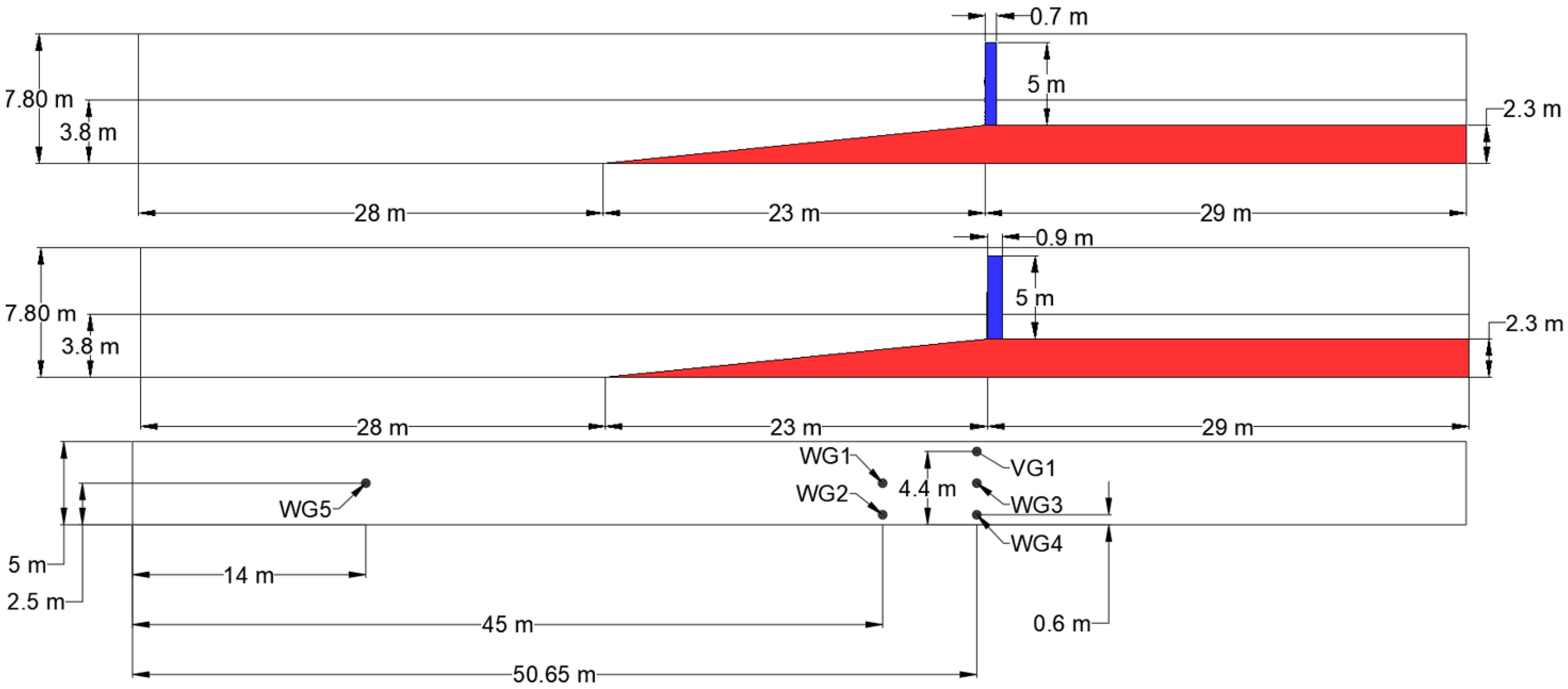
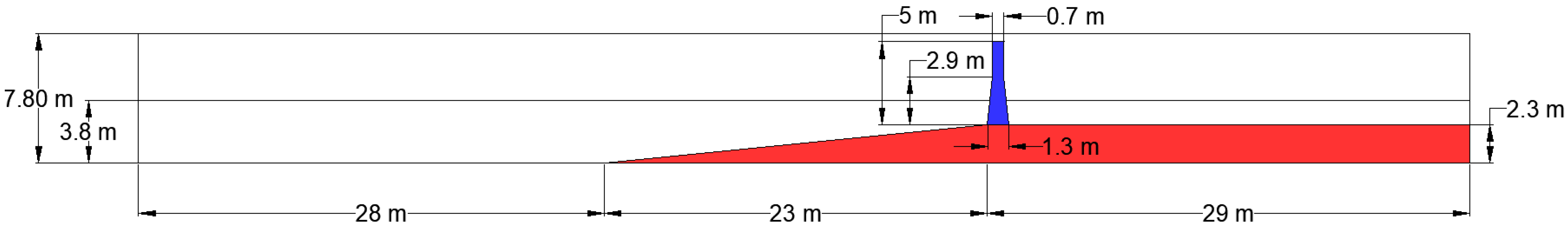
3.1. Experimental Set-Up

The experiments were conducted in the Large Wave Flume (GWK) of the Coastal Research Centre in Hannover, Germany by [5]. The flume length, width, and height were 309 m, 5 m, and 7 m respectively. A slope with an angle of 1:10 was installed in the flume, reaching 2.3 m height at the end of the plateau. The water depth adopted in the experiments was 3.8 m at the wave generator and 1.5 m on the plateau. A cylindrical substructure was installed at the edge of the slope with a diameter and length of 0.7 m and 5 m, respectively.

3.2. Model Description

To begin with, the numerical wave tank was created with the use of OpenFoam utility BlockMeshDict. The geometry of the cylindrical and conical substructures was created in SolidWorks in stereolithography files. Afterwards, with the OpenFoam utility snappyHexMesh, an unstructured mesh was created, and all the geometries were placed in the computational domain.

A scaled NWT with length, width, and height of 80 m, 5 m, and 7.8 m respectively, was developed as an equivalent to the experiment. Two vertical cylindrical substructures with diameters of 0.7 m and 0.9 m and a conical substructure with a diameter starting from 1.3 m to 0.7 m were placed where the wave breaks, as seen in Figure 1 and Figure 2, respectively. The free surface elevation η was measured at five numerical wave gauges (WG1, WG2, WG3, WG4, and WG5). The velocity in the direction of the wave propagation was measured with the velocity gauge VG1. The locations of the wave and velocity gauges are observed in Figure 1 and Table 2. Moreover, using the indicator phase function α, the free surface elevation in the z-direction was calculated for all the wave gauges.

Figure 1. Schematic representation of the Numerical Wave Tank (NWT) with the two vertical cylindrical substructures: front view (top); top view (bottom).

Figure 2. Schematic representation of the NWT with the conical substructure: front view.

Table 2. Measuring positions for wave and velocity gauges.

Gauge	X (m)	Y (m)	Z (m)
WG1	45.00	0.60	-
WG2	50.65	0.60	-
WG3	45.00	2.50	-
WG4	50.65	2.50	-
WG5	14.00	2.50	-
VG1	50.65	4.40	2.60

Fourteen gauges were placed near the substructures along the z direction every 30°. The details of the fourteen gauges are shown in Figure 3 and Table 3.

Figure 3. Schematic representation of the gauges near the substructures along the z direction every 30°.

Table 3. Measuring positions for gauges placed near the substructures along the z-direction.

Gauge Number	X (m)	Y (m)	Z (m)	Distance from the Slope
G1	50.98125	2.49375	2.40625	Near-bottom height
G2	50.98125	2.49375	2.60625
G3	50.98125	2.49375	2.80625
G4	50.98125	2.49375	3.05625	Half-distance between the slope and free surface
G5	50.98125	2.49375	3.70625	Near the free surface height
G6	50.98125	2.49375	3.80625
G7	50.98125	2.49375	3.90625
G8	50.98125	2.49375	4.70625	At wave-breaking height
G9	50.98125	2.49375	4.80625
G10	50.98125	2.49375	4.85625
G11	50.98125	2.49375	4.90625
G12	50.98125	2.49375	4.95625
G13	50.98125	2.49375	5.00625
G14	50.98125	2.49375	5.10625

The velocity and dynamic pressure were measured near the vertical cylindrical substructures every 30°. The details of the measuring positions are shown in Table 4.

Table 4. Measuring positions around the substructures.

Degrees	X (m)	Y (m)	Z (m)
0°	50.98125	2.49375	-
30°	51.03065	2.68438	-
60°	51.16563	2.81935	-
90°	51.34375	2.86875	-
120°	51.53438	2.81935	-
150°	51.66935	2.68438	-
180°	51.71875	2.49375	-
210°	51.66935	2.31563	-
240°	51.53438	2.18065	-
270°	51.34375	2.13125	-
300°	51.16563	2.18065	-
330°	51.03065	2.31563	-

For all the simulations, the incident wave period was T = 4.0 s, the incident wave height was H = 1.3 m, and the depth of the water was d = 3.8 m. In Table 5, all the wave parameters are presented. A fifth-order Stokes theory was sufficient for the wave generation considering all the above parameters.

Table 5. Incident wave conditions.

H (m)	T (s)	α (deg)	L (m)	ξ	Type of Breaker
1.3	4.0	5.71	20.53	0.397 < 0.5	Spilling

In order to determine the type of wave breaking, the Iribarren number (ξ) is required. The Iribarren number for periodic waves generating on a plane beach is defined as follows.

$$\mathsf{\xi }=\frac{\tan \mathsf{\alpha }}{\sqrt{\mathrm{H}/\mathrm{L}}}$$

(20)

where α is the bottom angle slope, H is the wave height, and L is the wavelength, which was calculated from Equation (21).

$$\mathrm{L}=\frac{\mathrm{g}{\mathrm{T}}^2}{2\mathsf{\pi }}\tanh \left(\frac{2\mathsf{\pi }}{\mathrm{L}}\mathrm{d}\right)$$

(21)

when the Iribarren number is ξ < 0.5, it is a spilling breaker and when is 0.5 < ξ < 3.3, it is a plunging breaker. Spilling breakers were generated in the numerical wave tank because the Iribarren number was 0.397, which is consistent with the observation in the experimental results provided by [5].

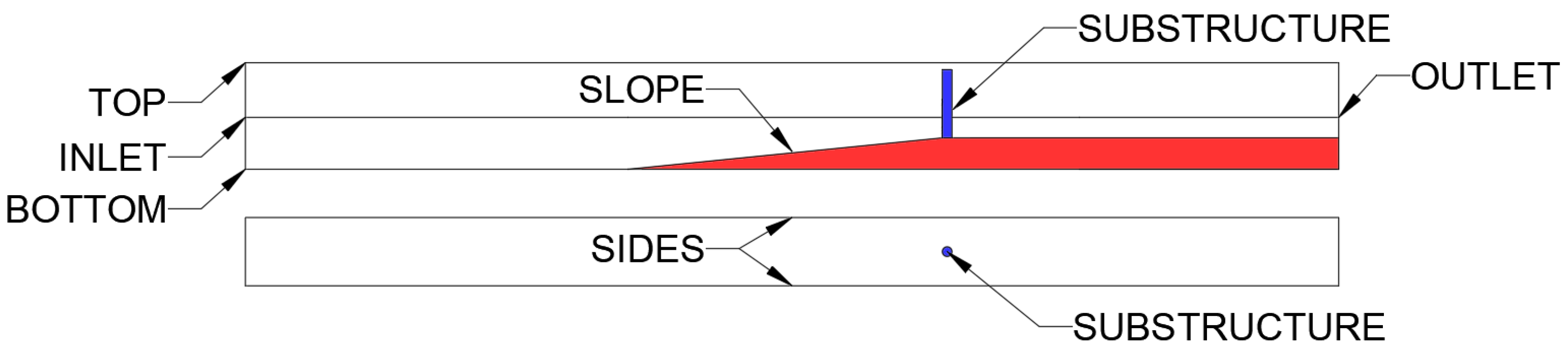
3.3. Boundary Conditions

In the present study, the boundary conditions included the inlet, outlet, top, bottom, sides, slope, and substructure. The NWT boundaries are shown in Figure 4.

Figure 4. Numerical Wave Tank Boundaries.

Initially, for the wave generation and wave absorption, the IHFOAM wave generation tool was used, developed by [20]. Wave generation and active wave absorption were activated at the inlet, while only wave absorption was activated at the outlet. The wave absorption was created based on shallow water theory to restrict the impact of the reflected waves in the direction of the wave propagation. The dynamic pressure P_rgh, k, and ω were defined with the normal zero-gradient boundary condition at the outlet region. Wall functions were activated for the NWT boundaries such as the slope, substructure, bottom, and sides according to the k−ω SST turbulence model. Furthermore, a fixed value (Dirichlet boundary condition) was defined for the velocity (0 m/s in the three directions), and a zero-gradient was used for the volume fraction. The fixedFluxPressure boundary condition was used for all boundaries except the top boundary for the dynamic pressure P_rgh. The FixedFluxPressure boundary condition is related to the zeroGradient and it was employed in circumstances where body forces such as gravity and surface tension were calculated in the solution equations. The totalPressure boundary condition was set for the pressure at the top boundary. The totalPressure boundary condition specifies that when there is outflow, the pressure is equal to the total pressure, and when there is inflow, the pressure is calculated from the local velocity and a specified total pressure expressed as illustrated below.

$$\mathrm{P}={\mathrm{P}}_0-0.5{\mathrm{u}}^2$$

(22)

where P₀ is the total pressure.

The “pressureInletOutletVelocity” boundary condition was set at the top boundary for the velocity, which applies zeroGradient to all components, except the tangential component where there is inflow, where a fixed value condition was used. In addition an “inletOutlet” boundary condition was set for the volume fraction at the top boundary, which permits water to flow outside and air to flow inside the domain when required, as driven by the fixed total pressure value specified. The details of the boundary conditions are shown in Table 6.

Table 6. Boundary conditions used in all simulation cases.

	Inlet	Outlet	Slope/Ground/Substructure	Sides	Top
U	Wave Velocity	Wave Velocity	Fixed Value	Slip	Pressure Inlet Outlet Velocity
Prgh	Fixed Flux Pressure	Fixed Flux Pressure	Fixed Flux Pressure	Fixed Flux Pressure	Total Pressure
Alpha	waveAlpha	Zero Gradient	Zero Gradient	Zero Gradient	Zero Gradient
K	Zero Gradient	Zero Gradient	Kqr Wall Function	Slip	Inlet Outlet
Omega	Inlet Outlet	Inlet Outlet	Omega Wall Function	Slip	Inlet Outlet
Nut	Calculated	Calculated	Nutk Wall Function	Slip	Calculated

3.4. Discretization Schemes

For the pressure and velocity coupling, the PIMPLE algorithm with three correctors was employed. A preconditioned bi-conjugate gradient (PBiCG) linear solver for asymmetric matrices using DILU as a preconditioner, based on simplified incomplete LU factorization for asymmetric matrices, was employed to solve for the velocity. A generalized geometric-algebraic multigrid (GAMG) solver was utilized for pressure calculations, using DIC as a preconditioner, based on the simplified scheme of incomplete Cholesky factorization for symmetric matrices.

3.5. Simulation Cases

In this present paper, three simulations were performed with different conical and cylindrical structures. The details of the domain discretization are presented in Table 7.

Table 7. Simulation discretization details.

Case	Simulation	Cells	Wave Generation	Near Substructure
1	Conical substructure	4,017,940	0.1 × 0.1 × 0.1 m3	0.0125 × 0.0125 × 0.0125 m3
2	Cylindrical substructure 0.7 m	3,764,981	0.1 × 0.1 × 0.1 m3	0.0125 × 0.0125 × 0.0125 m3
3	Cylindrical substructure 0.9 m	4,111,755	0.1 × 0.1 × 0.1 m3	0.0125 × 0.0125 × 0.0125 m3

4. Result and Discussion

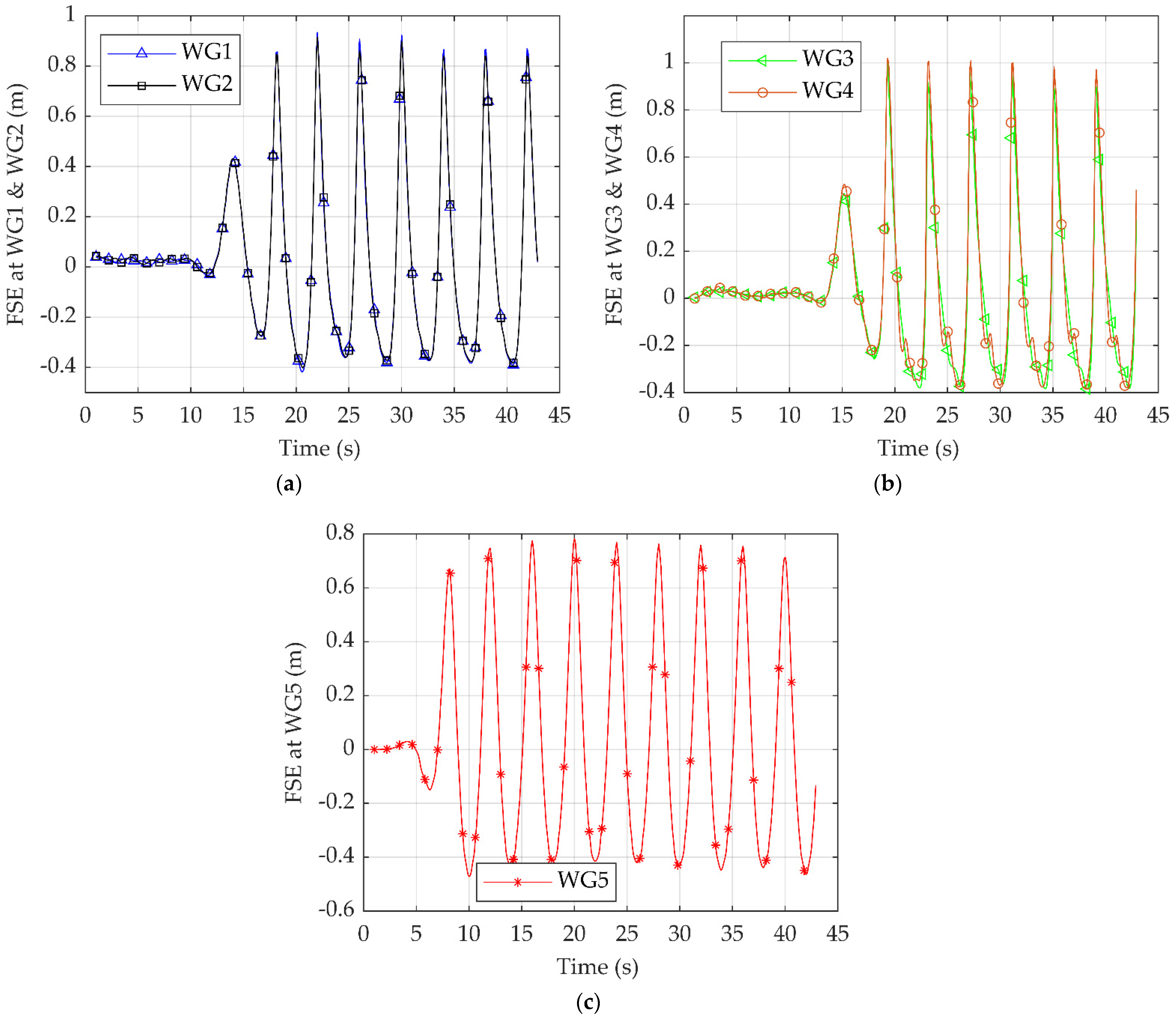
4.1. Wave Generation Capabilities

In an effort to validate the wave generation and the ability of the models to transport the wave without excessive dissipation, the simulated wave surface elevation was compared across five different numerical wave gauges to ensure that the same wave was generated along the NWT. The details of the different wave gauges involved in this study are presented in Table 2 and Figure 5a–c. In addition, the mean incident wave height for all the wave gauges is displayed in Table 8.

Figure 5. Free surface elevation at wave gauges for: (a) Wave Gauge 1 (WG1), WG2 (b) WG3, WG4, and (c) WG5.

Table 8. Wave-generation capabilities at different wave gauges in the Numerical Wave Tank (NWT).

Wave Gauge	Dimensionless Distance from the Wave Generation	Mean Peak Height (m)	Mean Trough Height (m)	Mean Incident Wave Height (m)	Difference from the Theoretical Value (%)
WG1	0.5625	0.8918	−0.3844	1.2762	1.83
WG2	0.5625	0.8658	−0.3771	1.2443	4.39
WG3	0.6331	0.9402	−0.3782	1.3183	1.41
WG4	0.6331	0.9983	−0.3721	1.3704	5.41
WG5	0.1750	0.7591	−0.4231	1.1910	8.39

WG1 and WG2 were located at a dimensionless distance 0.5625 from the wave generation. Conversely, the y-direction of WG1 was near the wall, whereas that of WG2 was at the centre of the NWT. The agreement between the two wave gauges was very good based on the difference from the theoretical values varying between 1.83% to 4.39%. In addition to the above-mentioned data, WG3 and WG4 were located at a dimensionless distance 0.6331 from the wave generation. However, the y-direction of WG3 was near the wall, whereas that of WG4 was at the centre of the NWT. The agreement between the two wave gauges was very good based on the difference from the theoretical values varying between 1.41% and 5.41%. Furthermore, the influence of the wave structure interaction was displayed near the trough of WG4 because the free surface elevation was fully developed. In contrast, in WG2, the influence of the wave structure interaction was not displayed due to the different locations of the wave gauges. Notably, the wave surface elevation in WG5 was not fully developed due to the proximity to the wave generation region with a deviation from the theoretical value at 8.39%.

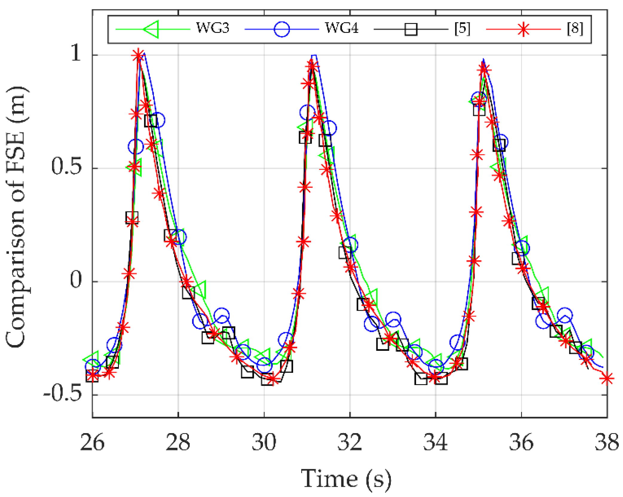
4.2. Comparison of the Free Surface Elevation with Available Experimental and Numerical Data

In Figure 6 and Table 9, the wave surface elevation at WG3 and WG4 was correlated with the numerical and experimental data provided by [5,8].

Figure 6. Comparison of the free surface elevation at WG3 and WG4 and the results of [5,8].

Table 9. Comparison of the free surface elevation at WG3 and WG4 and the results of [5,8].

Wave Gauge	Mean Peak Height (m)	Mean Trough Height (m)	Mean Incident Wave Height (m)	Difference from the Experimental Value (%)
WG3	0.9403	−0.3636	1.3040	6.00%
WG4	0.9967	−0.3738	1.3706	1.20%
[5]	0.9581	−0.4290	1.3871	-
[8]	0.9841	−0.4200	1.4042	1.23%

The above comparison yielded evidence suggesting that at the third gauge, the mean incident wave height was 6% lower than the experimental data provided by [5]. At the fourth wave gauge, the mean incident wave height agreed well with the experimental data, with only 1.20% deviation from the experimental data. The numerical simulations of Jose et al. [8] exhibited similar results for WG4, with only a 0.03% difference in the mean incident wave height. However, the influence of the wave structure interaction was not displayed in the numerical simulation of Jose et al. [8] probably due to the different wave generation technique employed in their study compared to the IHFOAM wave generation tool used in the present study.

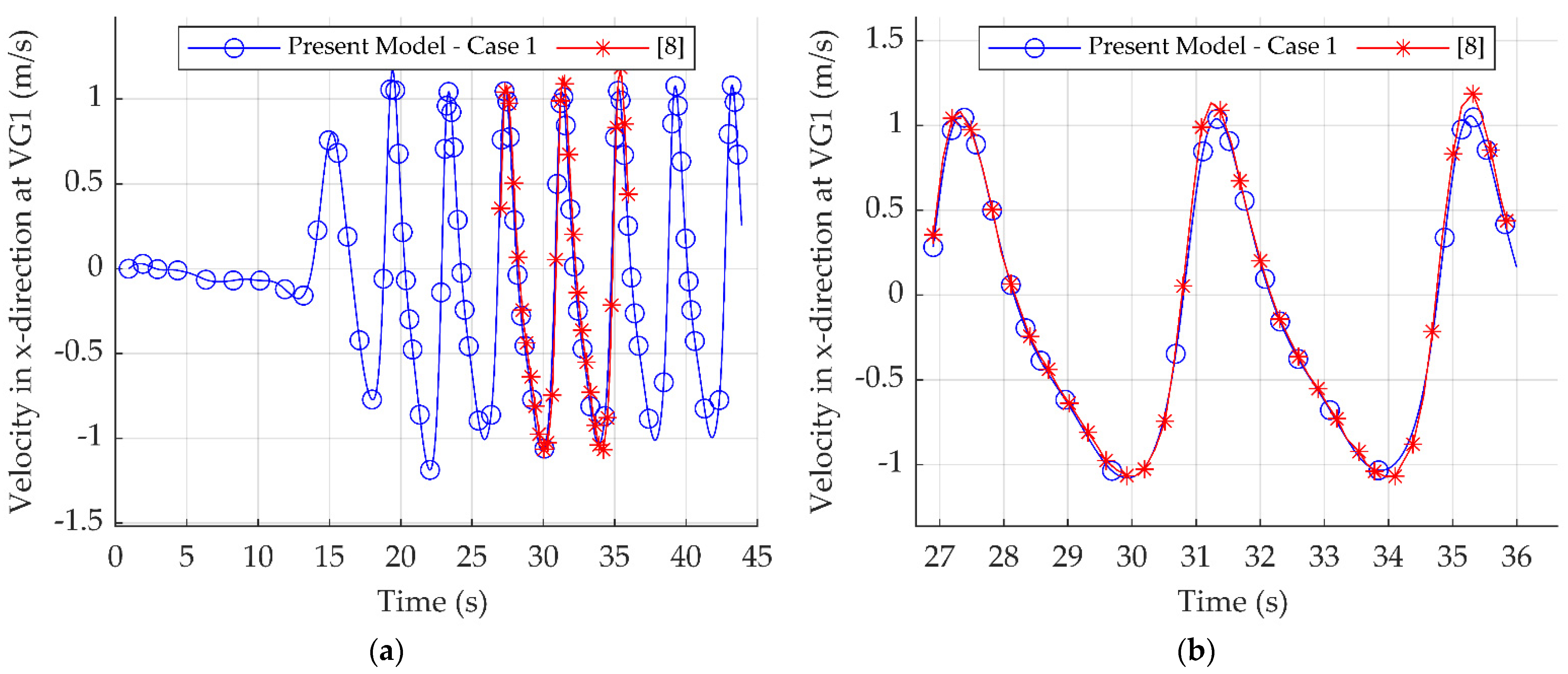
4.3. Comparison of the Velocity with Available Numerical Data

In Figure 7a,b and Table 10, the velocity in the x-direction at VG1 was correlated with the numerical data provided by [8].

Figure 7. Comparison of the velocity in the x-direction at VG1 and the results of [8] for: (a) the entire simulation time, (b) the numerical results simulation time.

Table 10. Comparison of the velocity in the x-direction at VG1 and the results of [8].

Wave Gauge	Mean Peak Velocity (m/s)	Mean Trough Height (m/s)	Mean Wave Velocity (m/s)	Difference (%)
VG1	1.0546	−1.0496	1.0521	4.32%
[8]	1.1335	−1.0656	1.0996	-

At the first velocity gauge, the mean wave velocity in the x-direction was 4.32% lower than the numerical data provided by [8]. While the agreement between the simulation data and the numerical data was very good, the wave generation technique employed in the numerical data by Jose et al. [8] was achieved with the wave2Foam library, in contrast to the IHFOAM technique applied in this paper. Moreover, as far as the velocity gauges from the experimental data are concerned, these were not included in the correlation as the velocity gauges were noisy.

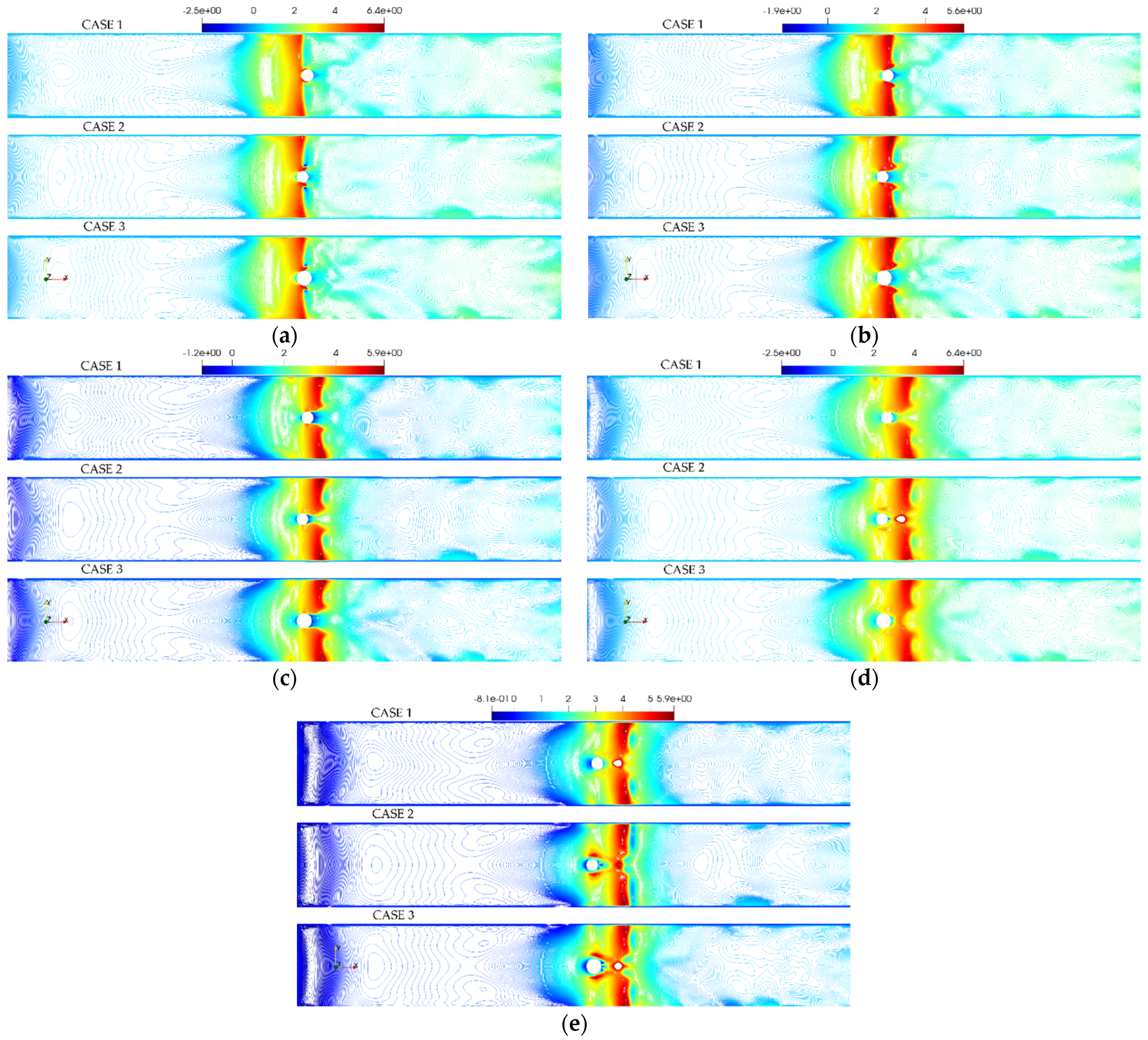
4.4. Velocity Distribution Near the Simulation Case 2 Substructure Over Time

In Figure 8a,b, the velocity in the x-direction at Gauges 1 and 9 was correlated with different angles around the substructure of Case 2 over time. Further details of the locations of the two gauges are presented in Table 3 and Table 4, respectively. As can be seen, Gauge 1 was located in the water phase, only 0.1 m above the plateau, whereas Gauge 9 was located in the air phase, 1 m above the mean water level. In Figure 8a, the maximum velocity in the x-direction was near 3 m/s and it was observed at 90°. Figure 8b shows that the maximum velocity in the x-direction was near 6m/s and it was also observed at 90°. Generally, the pattern of the velocity distribution around the substructure was repeated for all gauges. At first, when the wavefield hit the substructure, the water particles’ speed decreased to 0 m/s at 0°; this was the contact point. This location is also called the “stagnation point.” As the wave flowed from 0° around the substructure’s circumference, the velocity field increased along both sides because a smaller area of the substructure interrupted the flow field. It is apparent from Figure 8a,b that when the water particles were at 90°, the velocity was at a maximum level. Evidently, as the wave continued to flow around the substructure’s rear side, the velocity began to decrease and form another stagnation point.

Figure 8. Velocity in the x-direction at different angles around the substructure over time for: (a) Gauge 1 and (b) Gauge 9.

In Figure 9a,b, the velocity in the x-direction was correlated with different gauges. The gauges were placed at a 90-degree angle, where the velocity in the x-direction was highest, as shown in Figure 8, and the gauge heights differed in the z-direction. The details of the locations of the gauges are displayed in Figure 3 and Table 3, respectively. Gauges 1–4 were located in the water phase, whereas Gauges 5–7 were located near the free surface, and Gauges 8–14 were located near the wave breaking point above the mean water level. Figure 9a shows that Gauges 1–4 had small variations between them, with the maximum velocity in the x-direction near 2.5 m/s during wave breaking. In Gauges 5–7, the maximum velocity in the x-direction was about 3.5 m/s near the mean water level. In Gauges 8–14, where the gauge height was near the wave breaking, the maximum velocity in the x-direction was about 6 m/s.

Figure 9. Velocity in the x-direction for all the wave gauges at 90° over time for: (a) Gauges 1–7 and (b) Gauges 8–14.

4.5. Pressure Distribution Near the Simulation Case 2 Substructure Over Time

Figure 10 demonstrates the maximum pressure fluctuations at different locations around the substructure over time. It can be observed that the pressure variations around the substructure were similar to those of the velocity distribution values. Therefore, when the wave hit the structure, the dynamic pressure reached its peak value at 0° along the substructure’s front surface. Subsequently, the wave flowed from the high-pressure region to the low-pressure region, where the water particles moved along the cylindrical substructure circumference and gradually decreased. Near 135° around the foundation, the pressure value reached the minimum level. When the water particles continued to move around the substructure’s downstream side, the velocity began to slow down and form another stagnation point. These findings offer compelling evidence that additional peaks in dynamic pressure can be observed at the rear face of the substructure.

Figure 10. Dynamic pressure at Gauge 1 at different angles around the substructure.

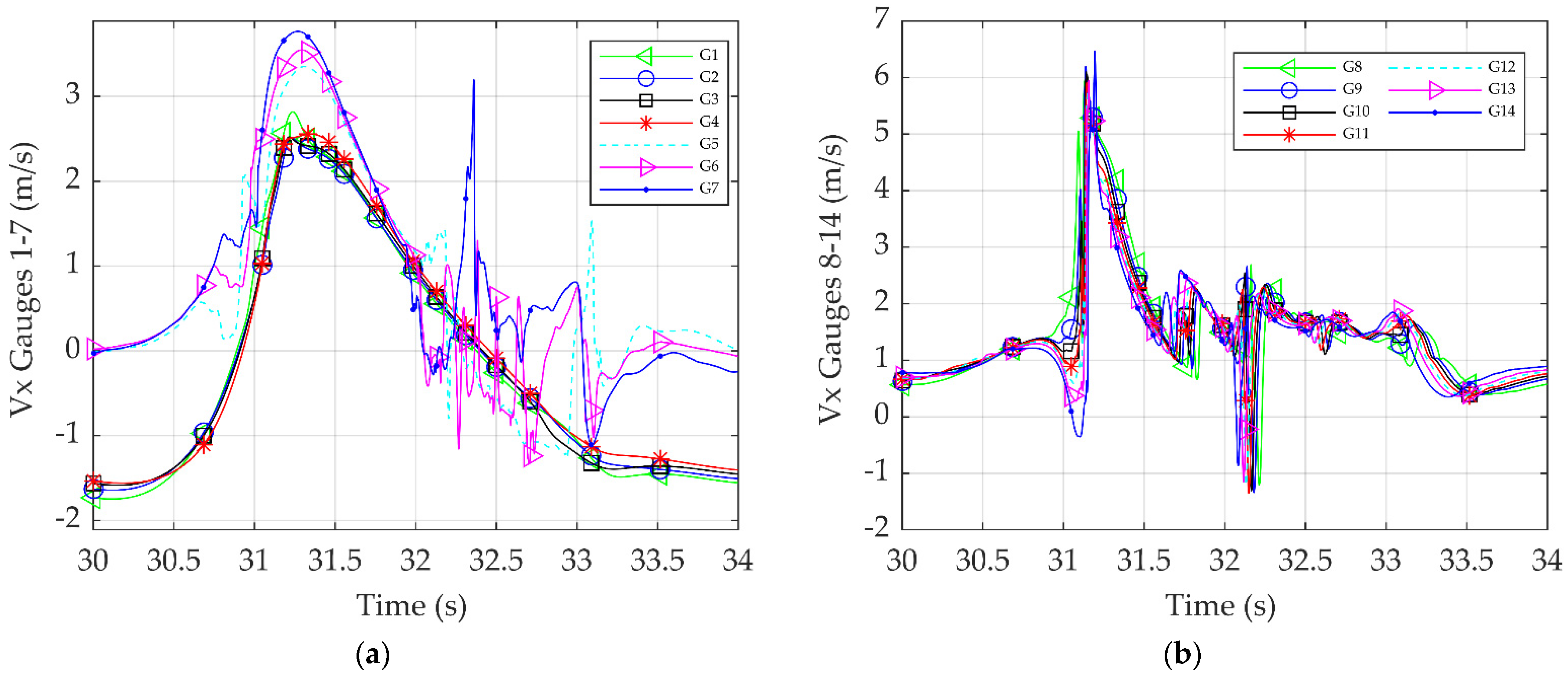
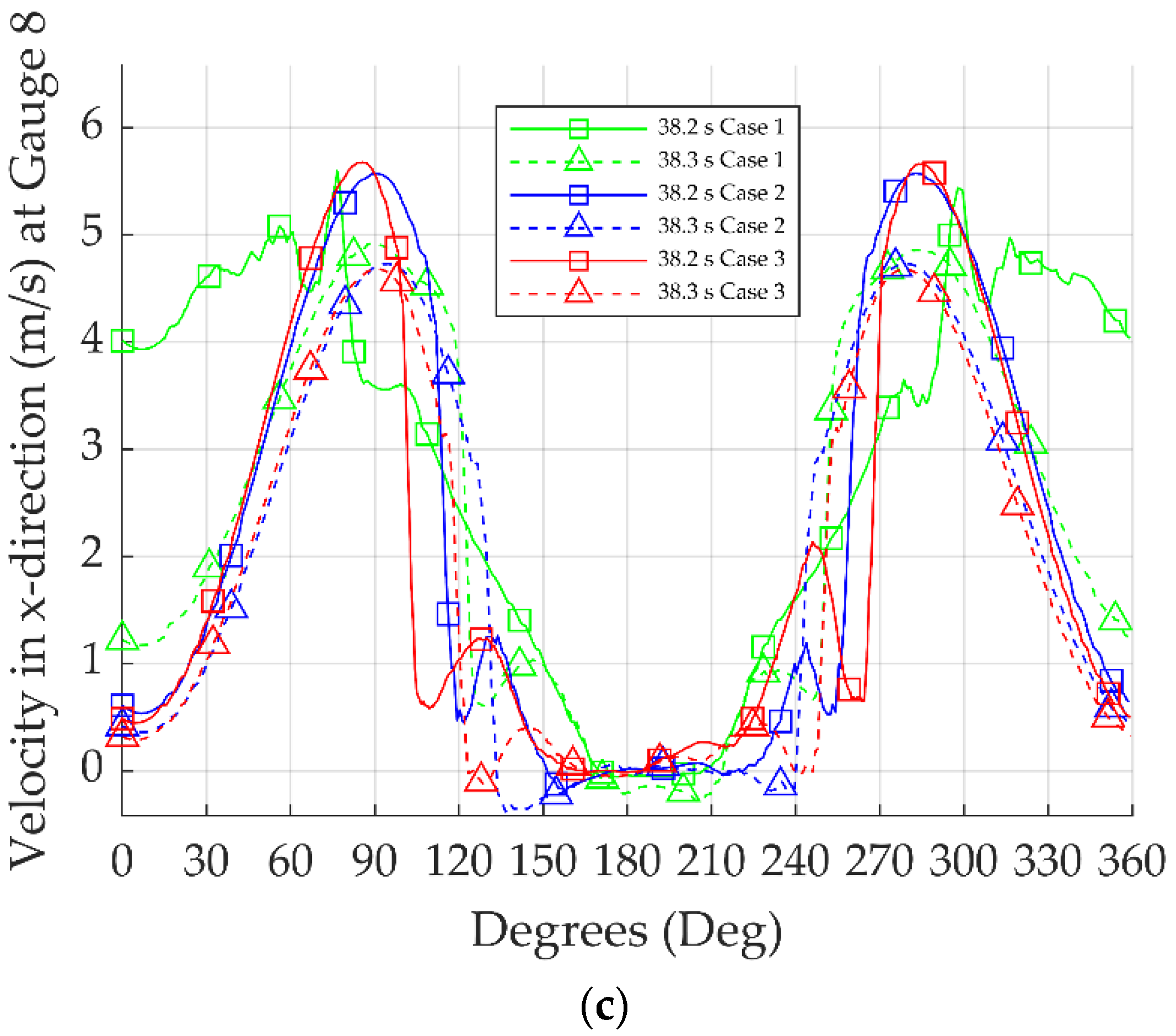
4.6. Comparison of the Velocity Distribution around Substructures at Different Heights

In Figure 11 and Table 11, the velocity distribution around the circumference of the substructures for all the simulation cases is compared during wave breaking at different heights.

Figure 11. Comparison of velocity distribution around substructures at different heights for (a) Gauge 2, (b) Gauge 6, and (c) Gauge 8.

Table 11. Comparison of the velocity distribution around substructures at different heights.

Simulation	Maximum Velocity at 38.2 s (m/s)	Difference (%)	Maximum Velocity at 38.3 s (m/s)	Difference (%)
At Gauge 2 height—Near the bottom
Case 1	1.288	41.640	1.739	25.490
Case 2	2.207	-	2.334	-
Case 3	1.853	16.040	2.199	5.780
At Gauge 6 height—Near the free surface
Case 1	2.645	16.690	3.234	7.920
Case 2	3.175	-	3.512	-
Case 3	3.060	3.620	3.397	3.270
At Gauge 8 height—Near the wave breaking
Case 1	5.596	0.420	4.918	4.020
Case 2	5.573	-	4.728	-
Case 3	5.676	1.850	4.681	1.010

In all simulation cases, the incident wave conditions were identical. An observation that can be made in Figure 11a is that the velocity distribution near the bottom was clearly affected by the different geometry of the substructures, with declinations between 25.5–41.6% in simulation Case 1 and 5.7–16% in simulation Case 3. In Figure 11b, the difference decreased near the free surface elevation, with values between 7.9 and 16.7% for simulation Case 1 and between 3.3 and 3.6% for simulation Case 3. In Figure 11c, it can be observed that near the wave breaking, the highest velocity in the x-direction was fairly close, marking a declination between 1–4%, although the diameter and the geometry of the substructures were different. On this account, the substructure’s velocity distribution did not change significantly with the increase in the substructure’s diameter near the wave breaking height. The substructure’s velocity distribution near the seabed was clearly affected by the different geometries of the substructures, especially in the conical shape, indicating large declinations. Moreover, the maximum velocity was noted at a different angle for the different substructures ranging from 90.7°–101.9° in Case 2 to 78.8°–85.5° in Case 3. Further to this, in Case 1, the velocity distribution probably changed due to the substructure having a conical shape. The breaker position was displaced further to the right than in the other two cases, and the maximum velocity was observed near 76.6°–89.2°.

In Figure 12, the velocity distribution of the substructures for all the simulation cases where the maximum velocity was observed at 0.9 m above the free surface was compared at various time steps during the wave breaking.

Figure 12. Comparison of velocity distribution in the x-direction for different substructures at various time steps for: (a) t = 31.2 s, (b) t = 31.3 s, (c) t = 31.4 s, (d) t = 31.5 s, and (e) t = 31.6 s.

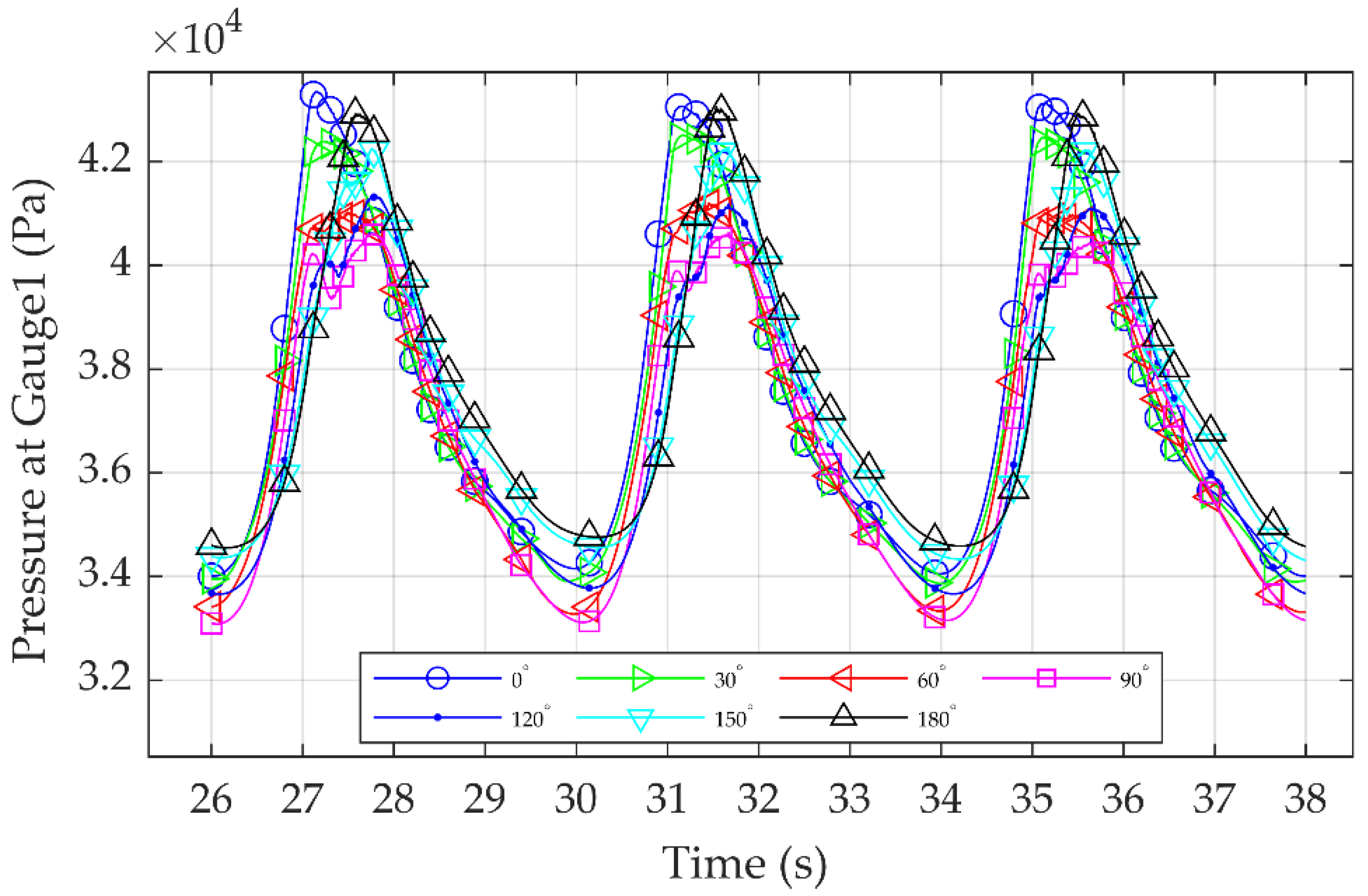
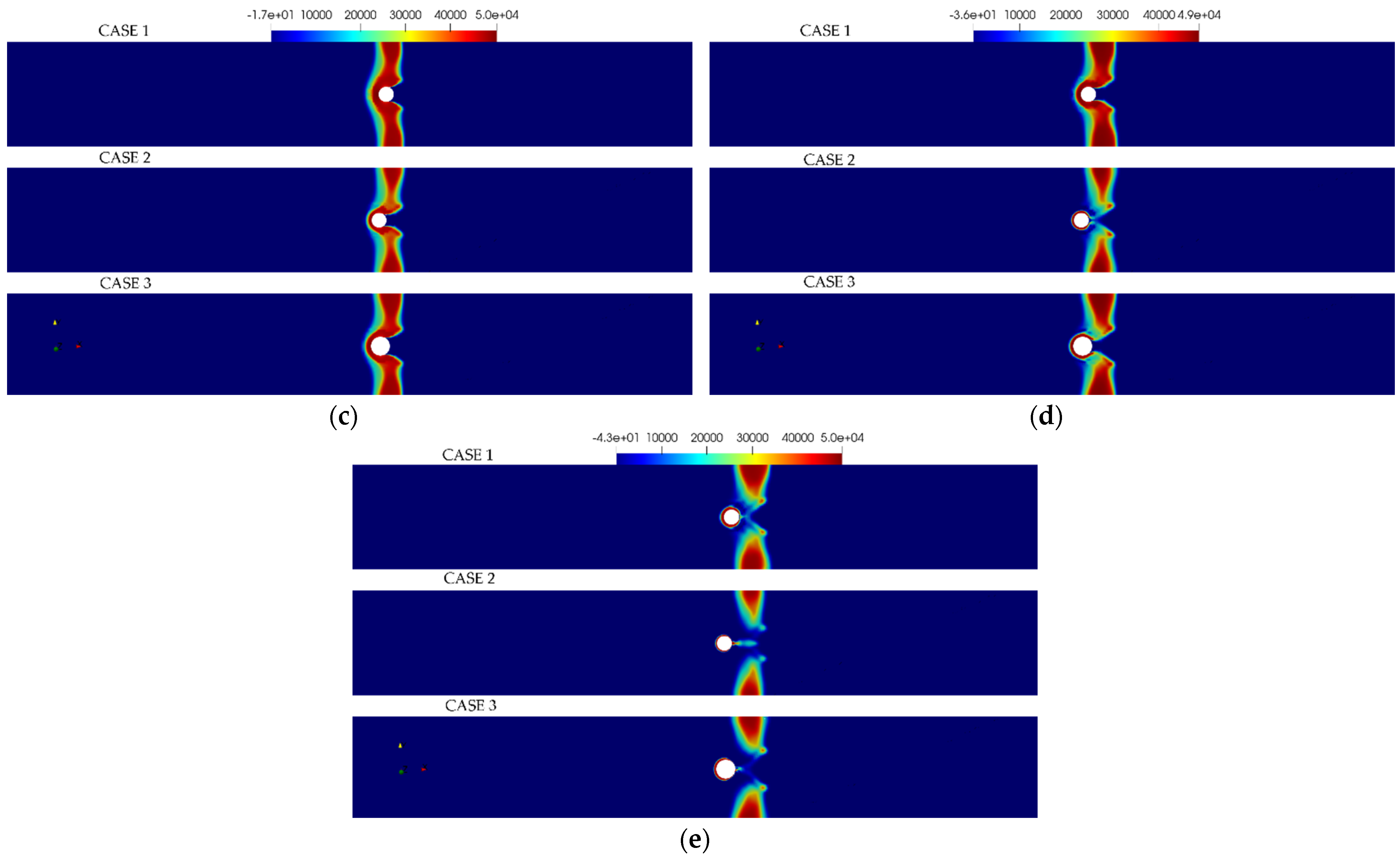
4.7. Comparison of the Pressure Distribution around Substructures at Different Heights

In Figure 13 and Table 12, the pressure distribution was compared for all the simulation cases around the circumference of the substructures during the wave breaking at different heights.

Figure 13. Comparison of the pressure distribution around substructures at different heights, for: (a) Gauge 2, (b) Gauge 6, and (c) Gauge 8.

Table 12. Comparison of the pressure distribution around substructures at different heights.

Simulation	Maximum Pressure at 38.2 s (Pa)	Difference (%)	Maximum Pressure at 38.3 s (Pa)	Difference (%)
At Gauge 2 height—Near the bottom
Case 1	44,102.0	2.010	43,793.0	1.640
Case 2	43,233.0	-	43,086.0	-
Case 3	43,591.0	0.830	43,273.0	0.430
At Gauge 6 height—Near the free surface
Case 1	47,717.0	1.920	46,806.0	1.830
Case 2	46,816.0	-	45,963.0	-
Case 3	47,267.0	0.960	46,132.0	0.370
At Gauge 8 height—Near the wave breaking
Case 1	53,077.5	2.380	51,908.3	3.050
Case 2	54,371.3	-	50,373.3	-
Case 3	54,674.3	0.560	50,458.2	0.170

In all simulation cases, the incident wave conditions were identical. The highest dynamic pressure was fairly close in all simulations with a declination between 0.17–3.05%, although the diameter and the geometry of the substructures were different. Moreover, the dynamic pressure distribution around the substructure’s circumference did not change significantly with the increase in the substructure diameter.

To start with, the maximum pressure was noted at the substructure’s front face in all simulation cases because at this point, the water particles’ speed decreased to zero. As the wave traveled around the substructure, the velocity increased and at the same time, the pressure decreased. In Figure 13a, the dynamic pressure decreased until 178.8°–186.4° and then it started to increase. In simulation Case 2, at 38.3 s, there was an obvious increase in the dynamic pressure from 109.1° to 188.8°, and then a symmetrical behaviour was witnessed. This increase was observed only in simulation Case 2 and it refers to the start of the secondary load. This may have occurred due to the circumference of Case 2 being the smallest of all simulation cases; thus, the wave faster propagated along the rear of the cylindrical substructure. Consequently, the start of the secondary load occurred faster. Another observation was that the dynamic pressure did not decrease to zero because the location of the gauge was in the water phase and therefore it did not drop instantly to zero. In Figure 13b, the dynamic pressure decreased until another local peak of dynamic pressure occurred at 112.1°, 148.0°, and 123.8° for simulation Cases 1, 2, and 3 respectively. Subsequently, the pressure dropped rapidly to zero at 38.2 s because Gauge 8 was just above the free surface. As aforementioned in the previous timestep, at 38.3 s, for simulation Cases 1 and 3, a similar behaviour was observed. For simulation Case 2, however, the dynamic pressure did not drop to zero. This may have occurred because the circumference in Case 2 was smaller than that in all of the simulation cases. A reasonable deduction would then be that the wave propagated faster along the rear of the substructure, and the secondary load started at a faster time than in the other cases. In Figure 13c, the dynamic pressure decreased until another local peak of dynamic pressure occurred from 94.7° until 119.3° for simulation Cases 2 and 3. In a subsequent step, the pressure dropped rapidly to zero. Furthermore, because the breaker location was displaced further to the right in Case 1 compared to the other cases, a delay in wave breaking was evident. Thus, at 38.2 s, the dynamic pressure distribution was different from the other cases and changed rapidly at 15°, from the maximum value, to zero at 48.6°. At 38.3 s, in all cases, the distribution of the dynamic pressure was similar. However, in Case 1, the dynamic pressure value was higher because the wave breaking was delayed.

In Figure 14, the dynamic pressure distribution around the circumference of the substructures for all the simulation cases where the dynamic pressure was maximum at 0.9 m above the free surface was compared at various time steps during the wave breaking.

Figure 14. Comparison of the pressure distribution for different substructures at various time steps for: (a) t = 31.2 s, (b) t = 31.3 s, (c) t = 31.4 s, (d) t = 31.5 s, and (e) t = 31.6 s.

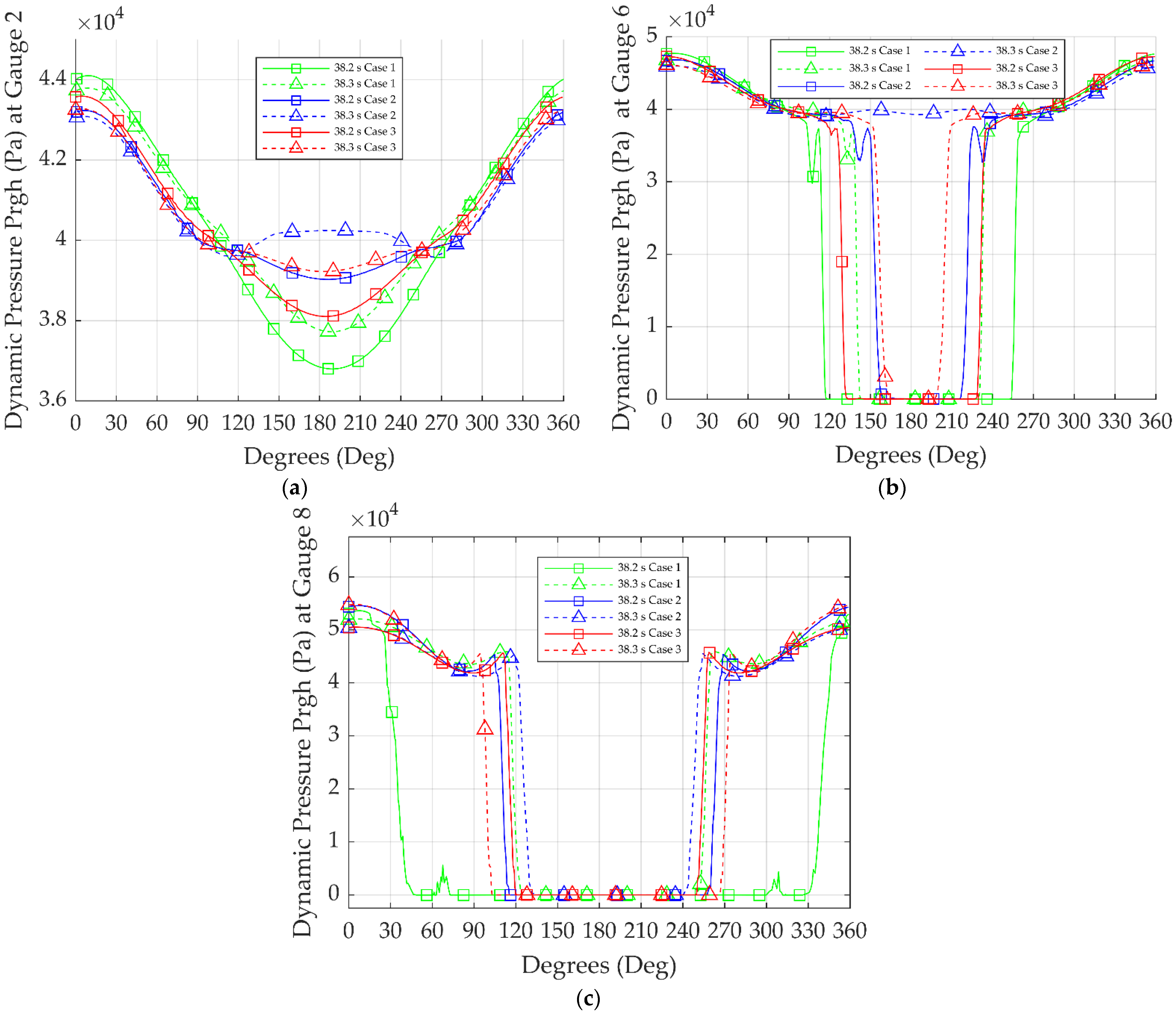
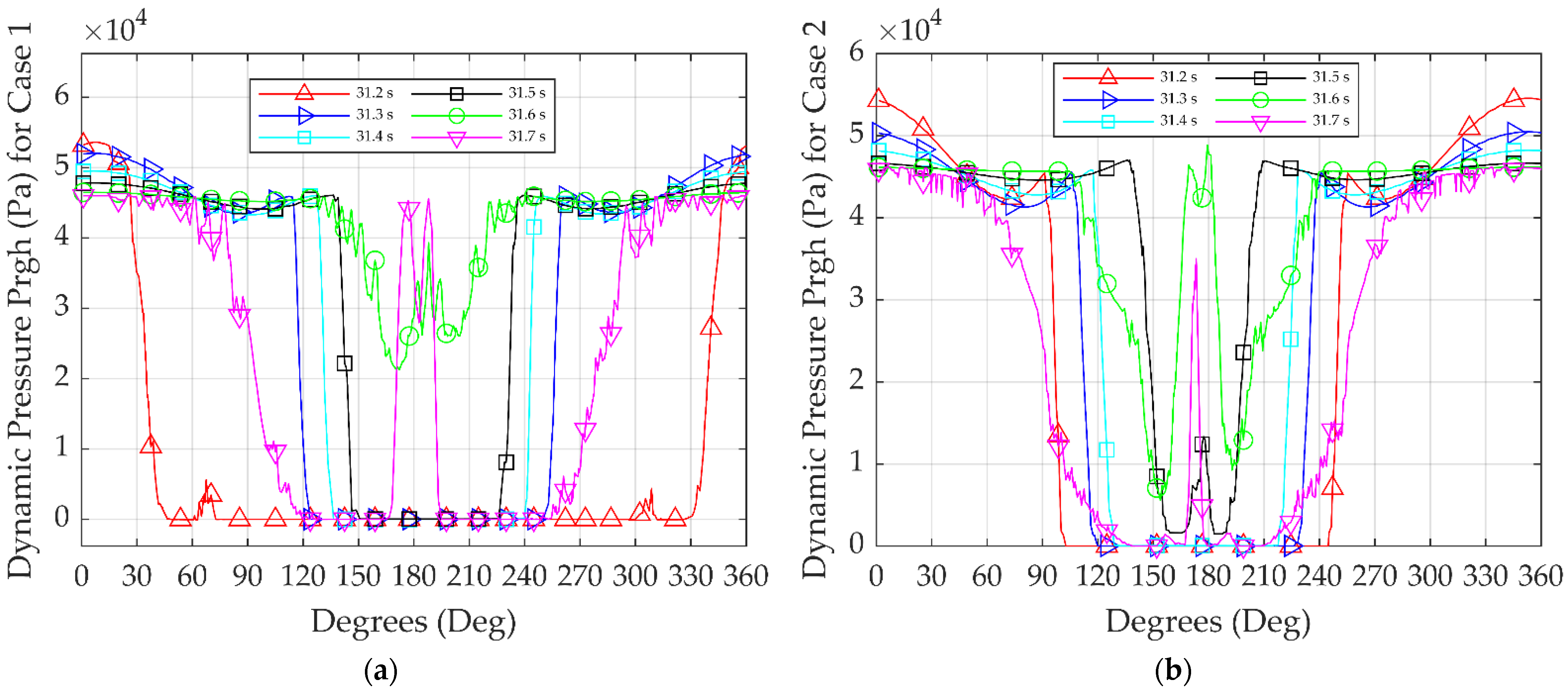
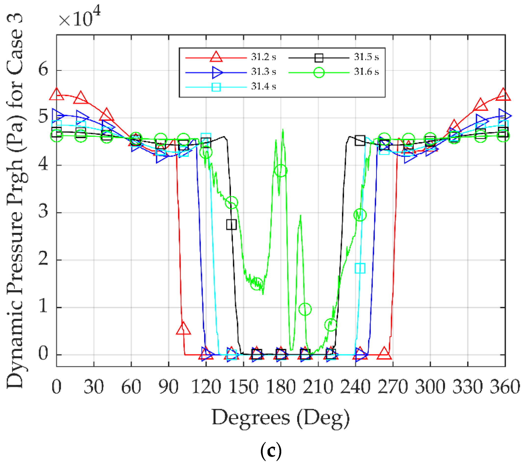
4.8. Dynamic Pressure Distribution around the Substructure at Different Time Steps

The dynamic pressure distributions around the substructure’s circumference at different time steps for all the simulation cases are presented in Figure 15.

Figure 15. Pressure distribution around the substructure at different time steps for: (a) Case 1, (b) Case 2, and (c) Case 3.

The pressure gauge’s angular position was set as the angle from 0° in the clockwise direction. The dynamic pressure at the substructure’s front point (0°) had a peak value at 31.2 s. It is fundamental to note that, simultaneously, the dynamic pressure decreased sharply from the peak value to zero from 0° to 90°. This difference can be interpreted using the properties of the flow field near the substructure. Firstly, when the wavefield hit the substructure, the water particles’ speed decreased to 0 m/s at 0°, while the dynamic pressure reached its maximum point. As the wave travelled around the cylindrical substructure circumference, the velocity field increased on both sides since a smaller area of the substructure interrupted the flow field, and the dynamic pressure decreased sharply to zero, from 0° to 90°. From 31.3–31.4 s, the dynamic pressure’s value was smaller than the peak value at the wave breaking at 31.2 s. At this point, the dynamic pressure decreased sharply to zero from 0° to 130° because the wave started to move away from the substructure’s front side. At 31.5 s, the secondary wave load was created near the substructure’s rear at 180°. At 31.6 s, the largest dynamic pressure was observed at the rear location of the substructure. Adding to this, at 31.7 s, the secondary load’s dynamic pressure had a smaller value compared to 31.6 s because the interaction between the fluid and the cylinder weakened.

Comparing all the simulation cases, it can be underlined that in Case 2, the start of the secondary load occurred faster due to the smaller circumference compared to the other substructures where the diameter was larger. It is crucial to mention that in Case 1 where the geometry of the substructure was conical, a delay in the presence of the primary and the secondary wave load was observed because the breaker location was displaced further right than in the rest of the cases.

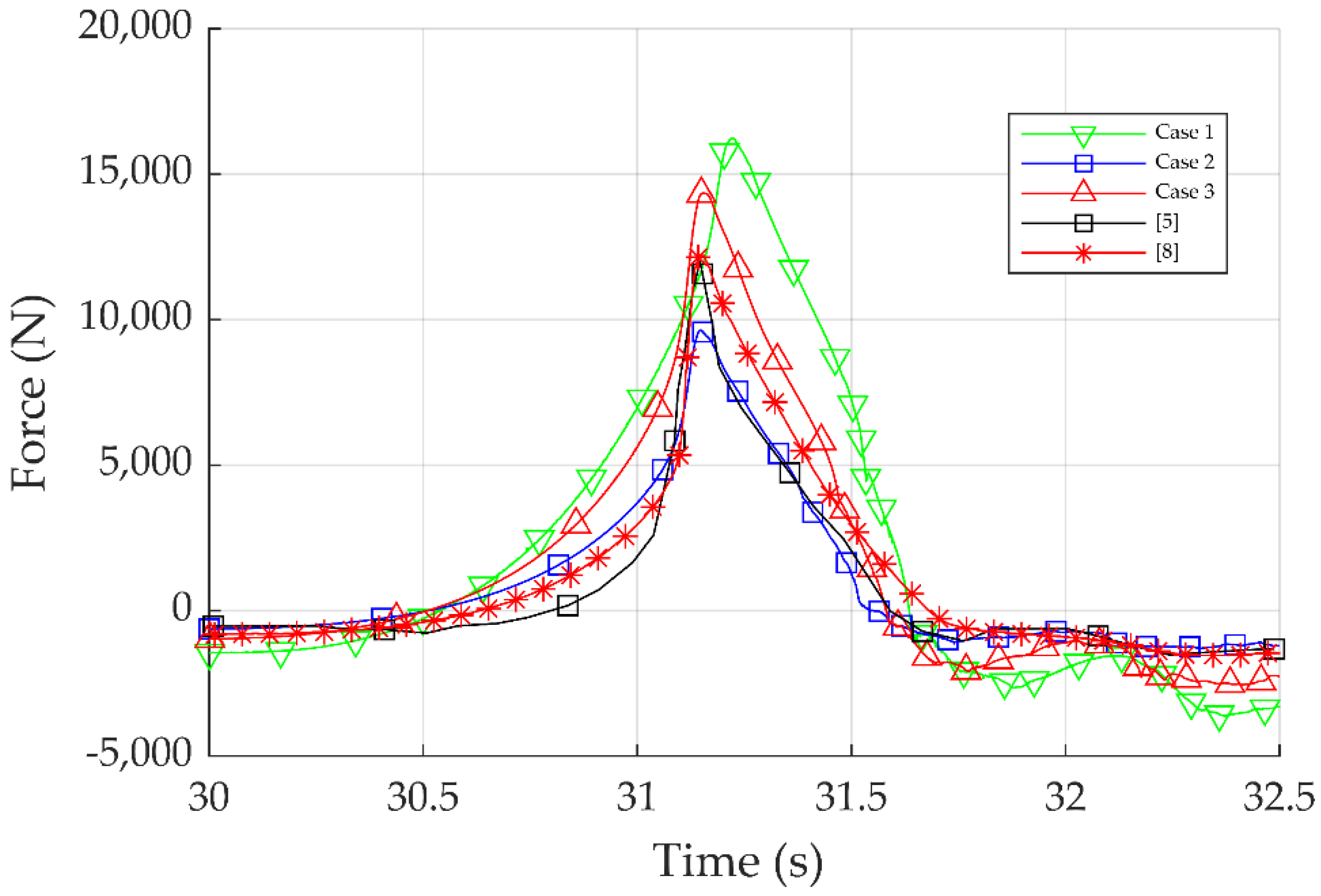
4.9. Breaking Wave Loads

Figure 16 and Table 13 show the primary wave load acting on different substructures for all simulation cases compared to the experimental and numerical data provided by [5,8].

Figure 16. Comparison of the magnitude of the primary wave load for all simulation cases and the results of [5,8].

Table 13. Comparison of the magnitude of the primary wave load for all simulation cases.

Simulation	Mean Value of the Primary Wave Load (N)	Difference (%)
Case 1	16,549.2	39.89
Case 2	10,179.3	13.95
Case 3	14,833.6	25.39
[8]	12,267.8	3.70
[5]	11,830.0	-

In a nutshell, the numerical results from simulation Case 2 had the same diameter as the experiment and the simulations from [8]. In simulation Case 2, the results had a lower primary wave load than the experimental results, with a declination of 13.95%. In contrast, the results provided by Jose et al. [8] are closer to the experimental data, probably due to the different numerical schemes employed in their study. Another finding worth mentioning is that in simulation Cases 1 and 3, the primary wave load increased when the diameter of the substructure increased. In addition, when the substructure was conical, it was observed that the wave breaking occurred with a delay because the breaker location was displaced further right and there was an increase of 62.57% in the primary wave load compared to the numerical results of simulation Case 2.

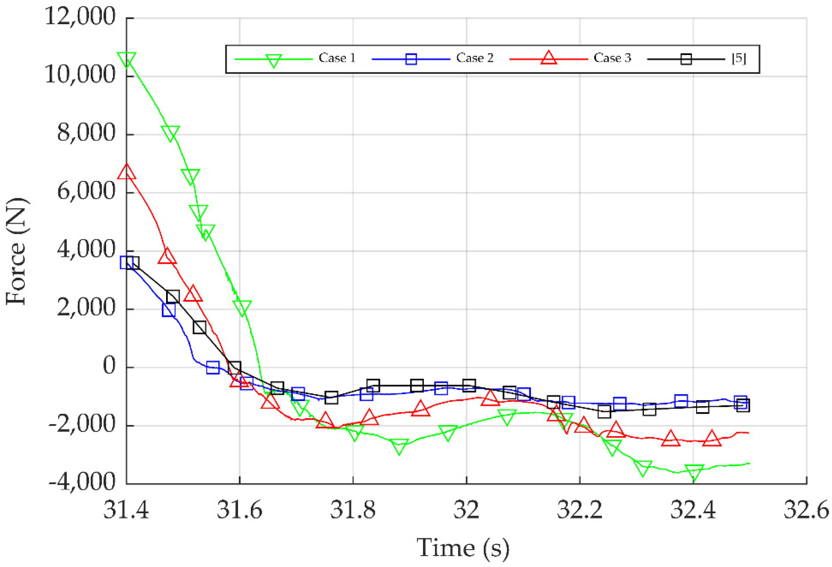
4.10. Secondary Wave Load

After the wave passed, a downstream gap was created at the rear of the substructure being filled from the diffracted waves. Subsequently, the diffracted waves created local pressure on the rear of the substructure. The local pressure appeared in the reverse direction of the wave propagation and exerted a negative force on the rear of the substructure. This effect was associated with the formation of the secondary load cycle, where the force reached a peak value and then disappeared. The secondary load had a smaller peak load in relation to the primary wave load. Nevertheless, it may have caused the higher-order excitations of such substructures. The effect of the secondary load was noticed at 31.7–32.4 s in all simulation cases. The magnitude of the secondary load cycle is presented in Figure 17.

Figure 17. The magnitude of the secondary load, F_secondary.

The comparison of the secondary load cycle for different substructures in the x-direction and the experimental results of Irschik et al. [5] is shown in Figure 18 and Table 14.

Figure 18. Comparison of the secondary load at the different substructures in the x-direction and the results of [5].

Table 14. Comparison of the magnitude of the secondary load for different cases.

Simulation	Magnitude of the Secondary Load (N)	Ratio of the Secondary Load to the Primary Load (%)
Case 1	1604	9.89
Case 2	473	4.91
Case 3	1200	8.37
[5]	619	5.16

As it can be seen, in Case 2, where the substructure’s diameter was similar to the experimental data, a very good agreement was observed compared to the numerical results of [5]. Likewise, the magnitude of the secondary load cycle for simulation Case 2 showed a strong agreement with the experimental data. In order to compare these values in a more objective manner, the ratio between the secondary load to the primary wave load is required. The percentage of the secondary load to the primary wave load for the experimental data was 5.16%. In contrast, for the same set-up, i.e., simulation Case 2, the ratio was 4.91% with a difference of only 4.84% from the experimental results ratio. Furthermore, the magnitude of the secondary load in the conical substructure was 3.39 times higher than that in Case 2, and the ratio of the primary-to-secondary wave load was double in the conical substructure compared to Case 2 which was 4.91%.

The secondary load peak values varied due to several stagnation points created for different substructure diameters. Comparing Cases 1, 2, and 3, it can be noted that the substructure diameter influenced the behaviour of the secondary load cycle. Accordingly, the wave reflection increased with the increasing diameter of the substructure. It can therefore be argued that the reflected waves’ impact became more extensive with the increasing substructure diameter, particularly in the substructure region. Consequently, when the substructure diameter increased, the secondary wave load also increased.

5. Conclusions

In this paper, the open-source CFD package OpenFoam with the k-ω SST model and the VOF method was applied to simulate breaking wave interactions with different cylindrical and conical substructures. The numerical results of the free surface elevation, primary wave load, and secondary load were compared to available experimental data provided by Irschik et al. [5] to validate the numerical model. The comparison drawn shows very good agreement between the present numerical results and the experimental data. Along these lines, the distributions of dynamic pressure and velocity around the circumference of different cylindrical and conical substructures were also studied. Following this, the wave breaking loads including the primary wave load and the secondary load were discussed for different cylindrical and conical substructures. Another important aspect of the study was whether the performance of a conical substructure would improve or deteriorate under the influence of a breaking wave load compared to a cylindrical one. Based on the simulations performed in this study and the observations made, it is not recommended to use a conical substructure in place of a cylindrical one. The main conclusions drawn from this study are the following:

• The evidence from this study suggests that the primary wave load increased when the diameter of the substructure increased. As aforementioned, the wave breaking occurred with a delay when the substructure was conical and the breaker location was displaced further to the right; an increase of 62.57% was noted in the primary wave load compared to the numerical results of simulation Case 2.
• The findings of this study also indicated that the diffracted waves created local pressure on the substructure’s rear side, which was related to the creation of the secondary load. The percentage of the secondary load ratio to the primary wave load for the experimental data and simulation Case 2 where the set-up was similar was only 4.84%. Notably, the substructure diameter influenced the behaviour of the secondary load cycle. As the diameter of the substructure increased, the wave reflection increased, and the secondary wave load also increased. The magnitude of the secondary load in the conical substructure was 3.39 times higher than that in Case 2, and the ratio of the primary-to-secondary wave load doubled in the conical substructure compared to Case 2, which was 4.91%. Consequently, the performance of a conical substructure will deteriorate under the influence of breaking wave load compared to a cylindrical one. The upshot of this, then, is that it is not recommend to use such a substructure in place of a cylindrical one.
• This study has also yielded evidence to suggest that the velocity distribution near the circumference of the conical substructure close to the seabed was clearly affected by the different geometry, with declinations between 25.5 to 41.6% compared to the cylindrical substructures. In contrast, the velocity distribution near the circumference of all substructures close to the wave breaking height did not change significantly with declinations between 1–4%. The diameter and the geometry of the substructures were different. It would also appear that the dynamic pressure distribution around the substructures did not change significantly with the increase in the substructures’ diameter and the change of the gauge height, although the incident wave conditions were the same for all cases.
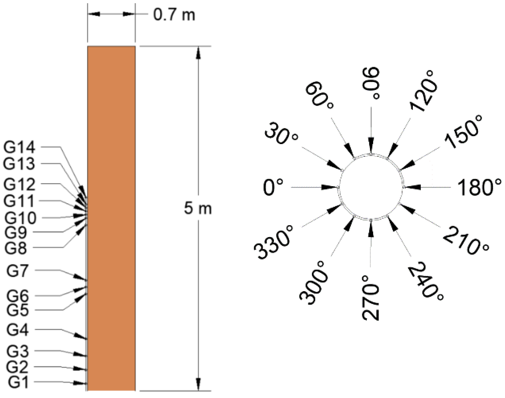
• This study has also provided results to show that when the wavefield hit the substructures, the velocity decreased to 0 m/s at 0°, which was the stagnation point. As the wave propagated around the substructure’s circumference, the velocity continued to increase on both sides until 90°, where the velocity reached its maximum level. As the wave continued to propagate around the substructure’s rear side, the velocity decreased and created another stagnation point.
• The study’s findings have also revealed that the dynamic pressure acting on the substructures reached its peak values at the front surface (0°). Then, the wave propagated from the high-pressure region to the low-pressure region. Near 135° around the cylinder circumference, the dynamic pressure value reached a minimum. As the wave propagated around the substructure’s rear side, the velocity decreased and another stagnation point was observed, therefore creating additional peaks of the dynamic pressure.

References

- Wind Europe. Wind in Our Sails: The Coming of Europe’s Offshore Wind Energy Industry; Wind Europe: Brussels, Belgium, 2011. [Google Scholar]
- Wind Europe. Offshore Wind in Europe: Key Trends and Statistics 2019; Wind Europe: Brussels, Belgium, 2020. [Google Scholar]
- Wienke, J.; Sparboom, U.; Oumeraci, H. Breaking Wave Impact on a Slender Cylinder. In Proceedings of the Coastal Engineering 2000; American Society of Civil Engineers (ASCE): Reston, VA, USA, 2001; pp. 1787–1798. [Google Scholar]
- Wienke, J.; Oumeraci, H. Breaking wave impact force on a vertical and inclined slender pile—Theoretical and large-scale model investigations. Coast. Eng. 2005, 52, 435–462. [Google Scholar] [CrossRef]
- Irschik, K.; Sparboom, U.; Oumeraci, H.; Smith, J.M. Breaking wave loads on a slender pile in shallow water. In Proceedings of the Coastal Engineering 2004; World Scientific Pub. Co. Pte Ltd.: Singapore, 2005; Volume 4, pp. 568–580. [Google Scholar]
- Liu, S.; Jose, J.; Ong, M.C.; Gudmestad, O.T. Characteristics of higher-harmonic breaking wave forces and secondary load cycles on a single vertical circular cylinder at different Froude numbers. Mar. Struct. 2019, 64, 54–77. [Google Scholar] [CrossRef]
- Qu, S.; Liu, S.; Ong, M.C.; Sun, S.; Ren, H. Numerical Simulation of Breaking Wave Loading on Standing Circular Cylinders with Different Transverse Inclined Angles. Appl. Sci. 2020, 10, 1347. [Google Scholar] [CrossRef]
- Jose, J.; Choi, S.-J.; Giljarhus, K.E.T.; Gudmestad, O.T. A comparison of numerical simulations of breaking wave forces on a monopile structure using two different numerical models based on finite difference and finite volume methods. Ocean Eng. 2017, 137, 78–88. [Google Scholar] [CrossRef]
- Liu, S.; Ong, M.C.; Obhrai, C. Numerical Simulations of Breaking Waves and Steep Waves Past a Vertical Cylinder at Different Keulegan–Carpenter Numbers. J. Offshore Mech. Arct. Eng. 2019, 141, 041806. [Google Scholar] [CrossRef]
- Chella, M.A.; Bihs, H.; Myrhaug, D. Wave impact pressure and kinematics due to breaking wave impingement on a monopile. J. Fluids Struct. 2019, 86, 94–123. [Google Scholar] [CrossRef]
- Kamath, A.; Chella, M.A.; Bihs, H.; Arntsen, Ø.A. Breaking wave interaction with a vertical cylinder and the effect of breaker location. Ocean Eng. 2016, 128, 105–115. [Google Scholar] [CrossRef]
- Brackbill, J.U.; Kothe, D.B.; Zemach, C. A continuum method for modeling surface tension. J. Comput. Phys. 1992, 100, 335–354. [Google Scholar] [CrossRef]
- Heller, V. Scale Effects in Physical Hydraulic Engineering Models. J. Hydraul. Res. 2011, 49, 293–306. [Google Scholar] [CrossRef]
- Hughes, S.A. Physical Models and Laboratory Techniques in Coastal Engineering; World Scientific: Singapore, 1993; Volume 7. [Google Scholar]
- Hirt, C.; Nichols, B. Volume of fluid (VOF) method for the dynamics of free boundaries. J. Comput. Phys. 1981, 39, 201–225. [Google Scholar] [CrossRef]
- Rusche, H. Computational Fluid Dynamics of Dispersed Two-Phase Flows at High Phase Fractions. Ph.D. Thesis, Imperial College of Science, Technology and Medicine, London, UK, 2002. [Google Scholar]
- Menter, F.; Ferreira, J.C.; Esch, T.; Konno, B. The SST Turbulence Model with Improved Wall Treatment for Heat Transfer Predictions in Gas Turbines. In Proceedings of the International Gas Turbine Congress 2003 Tokyo, Tokyo, Japan, 2–7 November 2003; pp. 1–7. [Google Scholar]
- Launder, B.; Spalding, D. The numerical computation of turbulent flows. Comput. Methods Appl. Mech. Eng. 1974, 3, 269–289. [Google Scholar] [CrossRef]
- Wilcox, D.C. Turbulence Modelling for CFD; DCW Industries: La Canada, CA, USA, 1998. [Google Scholar]
- Higuera, P.; Lara, J.L.; Losada, I.J. Three-Dimensional Interaction of Waves and Porous Coastal Structures Using OpenFOAM®. Part I: Formulation and Validation. Coast. Eng. 2014, 83, 243–258. [Google Scholar] [CrossRef]
Publisher’s Note: MDPI stays neutral with regard to jurisdictional claims in published maps and institutional affiliations. |
© 2021 by the authors. Licensee MDPI, Basel, Switzerland. This article is an open access article distributed under the terms and conditions of the Creative Commons Attribution (CC BY) license (https://creativecommons.org/licenses/by/4.0/).