Snowmelt-Driven Streamflow Prediction Using Machine Learning Techniques (LSTM, NARX, GPR, and SVR)

Abstract

Although machine learning (ML) techniques are increasingly popular in water resource studies, they are not extensively utilized in modeling snowmelt. In this study, we developed a model based on a deep learning long short-term memory (LSTM) for snowmelt-driven discharge modeling in a Himalayan basin. For comparison, we developed the nonlinear autoregressive exogenous model (NARX), Gaussian process regression (GPR), and support vector regression (SVR) models. The snow area derived from moderate resolution imaging spectroradiometer (MODIS) snow images along with remotely sensed meteorological products were utilized as inputs to the models. The Gamma test was conducted to determine the appropriate input combination for the models. The shallow LSTM model with a hidden layer achieved superior results than the deeper LSTM models with multiple hidden layers. Out of seven optimizers tested, Adamax proved to be the aptest optimizer for this study. The evaluation of the ML models was done by the coefficient of determination (R2), mean absolute error (MAE), modified Kling–Gupta efficiency (KGE’), Nash–Sutcliffe efficiency (NSE), and root-mean-squared error (RMSE). The LSTM model (KGE’ = 0.99) enriched with snow cover input achieved the best results followed by NARX (KGE’ = 0.974), GPR (KGE’ = 0.95), and SVR (KGE’ = 0.949), respectively. The outcome of this study proves the applicability of the ML models, especially the LSTM model, in predicting snowmelt driven discharge in the data-scant mountainous watersheds.

1. Introduction

Snowmelt is one of the major sources of fresh water in the world. Billions of people living in river basins originating from the snow-dominated Hindu Kush Himalayan (HKH) region, directly or indirectly rely on rivers for food, water, and electricity [1]. In this region, the accurate prediction of snowmelt runoff is crucial for effective water resource planning and management. However, the paucity of snow monitoring networks in the HKH region, due to geographical conditions and extreme weather, leads to inadequate ground truth information available for developing strategies for optimum water resource utilization. Remotely sensed snow cover and meteorological data are invaluable assets for snowmelt runoff modeling in the data-scant mountainous watersheds.

A number of models have been developed for accurate snowmelt runoff prediction based on various approaches. These models can be broadly classified into energy balance (EB) models, temperature index (TI) models, and data-driven (DD) models. EB models work on the principle of energy and mass conservation and require a profound understanding of complex processes including net radiation and heat exchange in a snowpack [2]. These models are computationally intensive and demand more data inputs [3], therefore, not suitable for operational forecasting in the data-scarce mountainous region. TI models use easily available air temperature data as a proxy to energy sources involved in the snowmelt process [4]. Therefore, TI models are simple and often used in operational forecasting, but they are not as good as sophisticated EB models [5]. Moreover, parameters of the TI models should be approximated through calibration. The process of finding suitable model parameters is tedious and also requires sufficient knowledge of the hydrological processes as well as catchment characteristics [6]. DD models such as machine learning (ML) can learn complex associations between inputs and outputs instantly and work with high model accuracy even without prior knowledge of the underlying processes [7]. However, despite its advantages, the application of ML models in snowmelt modeling is still scarce.

The history of ML and its applications, especially in different domains of water resource modeling, is well investigated in previous studies [7,8]. The majority of the ML applications are concentrated on artificial neural networks (ANNs), however, alternative ML methods, such as decision trees, support vector machines, and Gaussian process regression are also in practice. In a study, Callegari et al. [9] employed support vector regression (SVR) models for monthly snowmelt driven discharge forecasting in the Italian Alps using snow cover area (SCA) along with antecedent discharge and meteorological data. The SVR model predicted better than the benchmark linear autoregressive model. The applicability of SVR models in operational river discharge forecasting in Alpine catchments was further demonstrated by Gregorio et al. [10]. In a study, Uysal et al. [11] successfully employed a simple ANN model in the upper Euphrates basin of Turkey for one day ahead snowmelt forecasting. In the study, SCA, along with antecedent discharge, temperature, and precipitation as inputs showed excellent model efficiency (>93%). Moreover, the performance of the ANN model and the snowmelt runoff model (SRM) was compared. SRM [12] is a popular TI model which has been successfully applied to more than 100 basins for snowmelt modeling. The outcomes of the study [11] revealed that ANN models perform better than the widely-used SRM model.

Although traditional ANNs were very popular in the past, they were unable to retain temporal information, which is important in the case of time-series problems, such as hydrological forecasting. This drawback was solved by the recurrent neural network (RNN) [13]. However, RNNs were also not problem-free. The primary challenges to RNNs are exploding and vanishing gradient problems. A deep learning (DL) approach, known as long short-term memory (LSTM), overcomes the issues encountered by RNNs as well as preserves the long-term temporal information of the time-series data [14]. Due to the advancement in computer technology and the availability of remotely sensed data, DL methods are gaining popularity within the research and modeling community. Recent studies have shown great potentiality of the DL models, such as the LSTM model in rainfall-runoff modeling [15,16,17,18]. In the study by Kratzert et al. [15], two-layered LSTM with a dense layer was employed for rainfall-runoff modeling in the contiguous US catchments and among other things, they argued that the model could also mimic the snowmelt process by learning the relationship between precipitation during winter (cold temperature) and runoff in spring (warm temperature). However, in the Himalayan basins, where there is lack of sufficient meteorological stations and even if present, precipitation gauges considerably underestimate (up to 40%) the solid precipitation in high altitude region [19], precipitation data only may not be adequate for reproducing snow accumulation and melting process accurately. Moreover, precipitation and river discharge have no significant correlation whereas snow cover area (SCA) and river discharge are significantly correlated in the Central Himalayas [20]. Therefore, we utilized SCA as a key input to the LSTM model for predicting snowmelt runoff accurately; however, we also used precipitation data and compared the model performance for various inputs. Furthermore, Kratzert et al. [15] did not investigate the influence of hyperparameters (e.g., the number of LSTM layers and window size) on model performance but rather used some arbitrary values. Le et al. [17] and Fan et al. [16] emphasized the window size as an important hyperparameter to be tuned for best model performance, however, the effect of other hyperparameters, such as the number of LSTM layers and optimizers, were not evaluated.

This study aims to scrutinize the ability of the state-of-the-art deep learning LSTM network in modeling daily snowmelt runoff in a Himalayan basin. Furthermore, we evaluated the effect of various hyperparameters, including the number of LSTM layers and optimizers to achieve the best model performance. We developed three other ML models, namely, nonlinear autoregressive exogenous model (NARX), support vector regression (SVR), and Gaussian process regression (GPR) models and compared their performance. In this study, remotely sensed daily precipitation, temperature, and snow products along with the antecedent discharge data were used as inputs for one day ahead river discharge forecasting. The Gamma test (GT) was carried out to determine a suitable input combination for the model. The ML approach for operational river discharge forecasting will be useful in estimating water availability for reservoir management, water supply, irrigation, and hydroelectricity projects in the data-scarce mountain basins.

2. Materials and Methods

2.1. Study Area

Although the Himalayan region is a snow-glacier dominated region, snowmelt runoff modeling using ML models have not been conducted in this region. Therefore, Langtang basin (Figure 1), a snow-glacier dominated basin situated in Central Himalayas, Nepal is chosen for this study. The altitude of the study site lies in the range of 3647–7213 m above mean sea level. The catchment area is 354 km² comprising 110 km² of the glacier area. The glacier extent is derived from RGI-GLIMS version 6 [21]. Snow and glacier-melt is a significant contributor to the overall runoff in this watershed [22].

2.2. Hydrometeorological Data

The hydrological data gauged at the Kyangjing station (latitude 28.216°, longitude 85.55°) was received from the Department of Hydrology and meteorology (DHM), Nepal. The daily temperature data was derived from the 0.25° × 0.25° gridded APHRODITE product, APHRO_TAVE_MA_V1808, for the period 2002–2012 [23]. Previous studies have shown a good correlation (Spearman’s rho > 0.9) of APHRODITE products with ground observation in the Langtang basin [20]. Precipitation data, acquired from the tropical rainfall measuring mission (TRMM), with a spatial resolution of 0.25 degrees is used in this study [24]. 3B42RT TRMM datasets are completed in four phases. Precipitation related data are obtained from various sensors and the precipitation rate is computed. Infrared data, collected from the satellites, provides exceptional time-space coverage. These data are combined to provide the best precipitation estimate and finally, the rain gauge data are incorporated to produce the 3B42RT TRMM dataset. TRMM products have been widely used in the Himalayan region [25]. The product is available at https://pmm.nasa.gov [26].

2.3. Snow Cover

The moderate resolution imaging spectroradiometer (MODIS) product, MOD10A2 version 6 [27] is used for snow cover mapping. Several studies have verified the accuracy of MODIS datasets with ground observation. In a study, Stigter et al. [28] cross-checked the accuracy of MODIS snow data with in-situ snow observation in the Langtang basin and revealed an accuracy of 83.1%. The snow mapping algorithm uses MODIS band 4 and band 6 for determining the normalized-difference snow index [29]. In MOD10A2 product, a pixel is labeled as snow if snow cover is observed at least once in eight days, no snow if snow cover is absent in all eight days, and cloud if cloud cover is observed on all eight days. For this study, 496 images for the period (2002–2012) were downloaded from the National Snow and Ice Data Center (NSIDC) website (https://nsidc.org/data/mod10a2) [27]. The 30 m resolution Advanced Spaceborne Thermal Emission and Reflection Radiometer (ASTER) Global Digital Elevation Model (GDEM) is obtained from https://lpdaac.usgs.gov [30]. The boundary of the study area was delineated from the DEM. All MOD10A2 images were projected to World Geodetic System 1984 (WGS84), Universal Transverse Mercator (UTM) zone 45. The 8-day maximum SCA was extracted from projected snow images using the delineated boundary. Images with more than 10% cloud cover were discarded. Finally, the daily SCA for 365 days in a year was interpolated or extrapolated from the 8-day maximum SCA using the cubical spline method.

2.4. GT

For the DD models, input selection is an important task in the model development process [31], but it is often neglected. In most of the studies employing ML models, inputs were determined on an ad-hoc basis by trial and error method. In this study, we applied the GT [32], a non-parametric method to select input variables for a nonlinear and complex model. GT approximates the variance of the noise related to the output. Input variables are selected based on Gamma value and V-ratio. Input combination with the least Gamma value and V-ratio is considered best for the model. For the selection of a suitable input combination, 15 different input combinations of SCA, temperature, precipitation, and antecedent discharge were tested and the best input combination was determined using the winGamma^TM application (Cardiff University, University of Wales, Wales, UK) [33].

2.5. LSTM

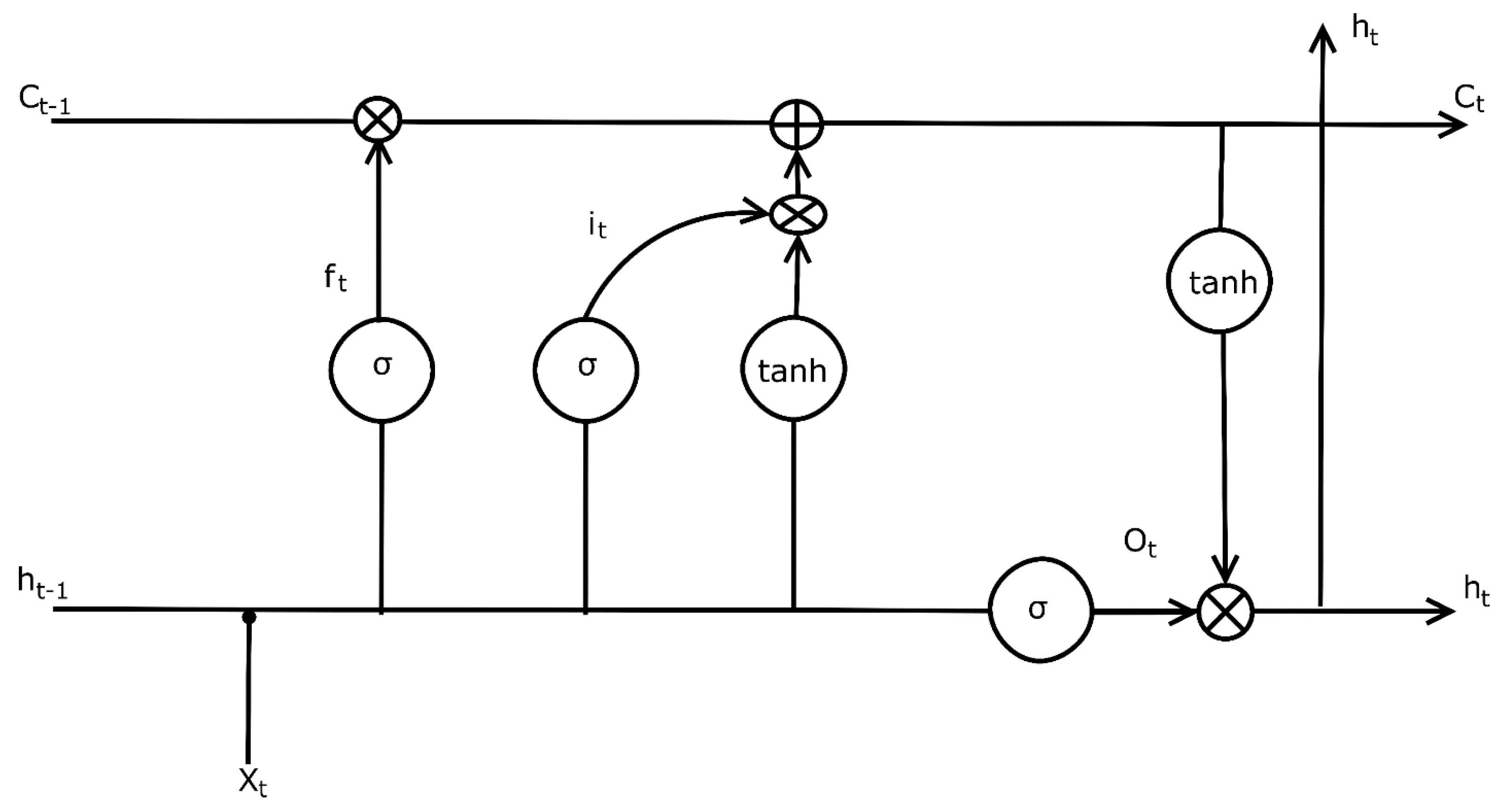
The LSTM, proposed by [14], is a specialized RNN able to learn and preserve long-term dependencies [15]. The unique feature of LSTM is the presence of a memory cell. In LSTM, adding or deleting the information in the cell is controlled by gates. LSTM has three types of gates, i.e., Forget, Input, and Output gates, to control the flow of information in the cell. The Forget gate governs the amount of information to remove from the previous cell state. The information to be introduced into the cell state is controlled by the input gate. Then, a vector of a candidate layer is generated which could be appended to the cell state. Then, the old cell state is adjusted to a new cell state according to the preceding two steps. The output layer opts information from the cell state to be used as output. The final LSTM layer at the final time step (n) passes the output (h_n) to a dense layer with a single output neuron where final streamflow (y) is calculated. Equations related to the LSTM cell are presented below.

$$\mathrm{Forget}\mathrm{gate}:f_t=\sigma (W_f{x}_t+U_f{h}_{t-1}+b_f)$$

(1)

$$\mathrm{Input}\mathrm{gate}:i_t=\sigma (W_i{x}_t+U_i{h}_{t-1}+b_i)$$

(2)

$$\mathrm{Potential}\mathrm{update}\mathrm{vector}:{\tilde{c}}_t=\tanh (W_{\tilde{c}}{x}_t+U_{\tilde{c}}{h}_{t-1}+b_{\tilde{c}})$$

(3)

$$\mathrm{Cell}\mathrm{state}:c_t=f_t\odot c_{t-1}+i_t\odot {\tilde{c}}_t$$

(4)

$$\mathrm{Output}\mathrm{gate}:O_t=\sigma (W_o{x}_t+U_o{h}_{t-1}+b_o)$$

(5)

$$\mathrm{Hidden}\mathrm{state}:h_t=\tanh (c_t)\odot o_t$$

(6)

$$\mathrm{Output}\mathrm{layer}:y=W_d{h}_n+b_d$$

(7)

$$\mathrm{Sigmoid}\mathrm{function}:\sigma (x)=\frac{1}{1+e^{-x}}$$

(8)

$$\mathrm{Tan}\mathrm{h}\mathrm{function}:\tanh (x)=\frac{e^x-e^{-x}}{e^x+e^{-x}}$$

(9)

where f, i, o are vectors representing forget, input, and output gates respectively, $c_t,{\tilde{c}}_t$ are vectors for the cell states and candidate values, $\sigma$ is the sigmoidal function, $\odot$ is element-wise multiplication, $x_t$ is input vector at time t, $W$ and $U$ are the weight matrix for input and hidden state, and b is the bias term. A classic LSTM cell is shown in Figure 2.

In this study, the LSTM model was developed using open-source Keras [34] with Tensorflow backend in Python. The presence of a large range of values in the dataset affects the learning skill as well as the convergence of the LSTM network during training. Therefore, for efficient learning and faster convergence, input and target data are rescaled to the range (0,1) by subtracting the minimum number and then dividing by the range, without altering the shape of the original distribution. Then, the time-series data is transformed to the supervised learning. The input data should be in a three-dimensional format (i.e., samples, time step, and features) for the LSTM model. For the final prediction, the output is retransformed to the original scale. The accuracy of the model is affected by the choice of hyperparameters [15,16,35,36]. Hyperparameters such as optimization algorithm, number of LSTM layers, hidden units, loss function, learning rate, batch size, and dropout are carefully selected based on performance or previous studies which is further discussed in Section 3.2.

2.6. NARX

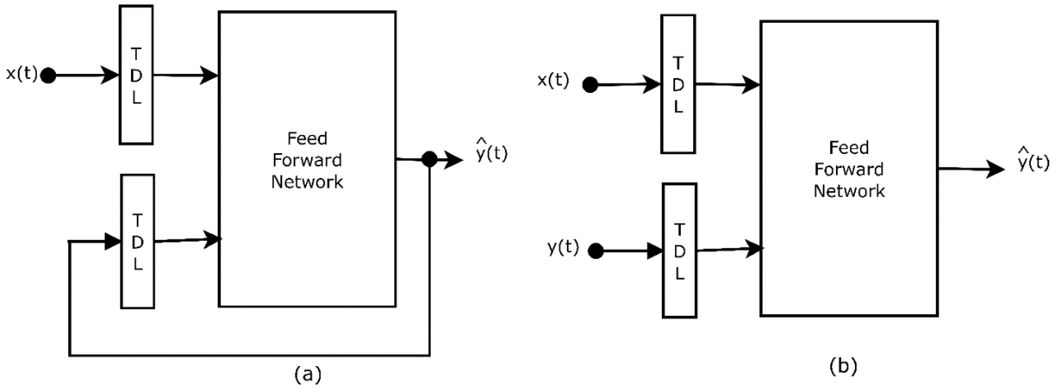
NARX, a recurrent dynamic network, is a powerful modeling tool with faster convergence and generalization than simple ANNs [37]. Several researchers have successfully employed the NARX model in hydrological modeling [38,39,40]; however, the potential of this model in snowmelt runoff modeling is yet unexplored. This model has feedback that links some of the network layers, so it is known as a recurrent dynamic network. Parallel (P) and series-parallel (SP) structures are two types of NARX model architecture (Figure 3). The SP model is preferred because it is a fully feedforward architecture and therefore, the backpropagation algorithm can be applied for training. Since the actual output is used, the SP model can produce accurate forecasts. The principal equation for the NARX model is

$$y(t)=f(y(t-1),y(t-2),\dots ,y(t-n_y),u(t-1),(u(t-2),\dots ,u(t-n_u))$$

(10)

where the predicted variable $(y)$ at timestep (t) is computed based on its previous values and previous values of exogenous input values$(u)$.

Training algorithm, number of hidden nodes, input delays, and feedback delays are the important parameters affecting the performance of the NARX model. The river discharge is predicted using the antecedent discharge and the exogenous inputs, including SCA, air temperature, and precipitation. The feedback delay was chosen by the autocorrelation function of the discharge data series. The number of hidden nodes and feedback delays was selected based on a trial and error method. Different training algorithms, such as Bayesian regularization (BR), Levenberg–Marquardt (LM), and scaled conjugate gradient (SCG) were applied for training the NARX model and their performance was compared. We used trainlm, trainbr, and trainscg functions in MATLAB version 2018b to train the model by LM, BR, and SCG method, respectively.

2.7. SVR

The support vector machine, introduced by Vapnik [41], is a standard ML tool for classification and regression. SVR is a nonparametric regression technique based on the Support Vector Machine. The SVR applies the principle of the structural risk minimization to recognize the pattern between predictor and predicted values, whereas, ANN use empirical risk minimization principle. In the SVM model, the learning function for inputs and outputs ((x₁, y₁), (x_n, y_n)) are created. The approximating function f(x) is given by:

$$f(x)={\displaystyle \sum }_{i=1}^l({\alpha }_i-{\alpha }_i^{*})K(x_i,x)+b$$

(11)

where $<x_i,x>$ denotes dot product of two vectors, x is the problem variable vector, b is the bias,${\alpha }_i$ and ${\alpha }_i^{*}$ are dual variables. Various studies have confirmed that the radial basis function (RBF) performs better than other kernel functions [42]. Therefore, in this study, the Gaussian RBF kernel function is used in the SVM model, which is defined as follows:

$$K(x,x_i)=exp(-\Vert x-x_i{\Vert }^2)$$

(12)

For the SVR model with the Gaussian RBF kernel function, the penalty parameter (C) and epsilon ($\epsilon$) are the important parameters that are determined by the trial and error method in this study.

2.8. GPR

The GPR model is a kernel-based probabilistic model. Gaussian processes can also be viewed as the Bayesian version of the SVM methods. They are flexible and simple to implement methods appropriate for problems related to classification and prediction [43]. Unlike ANNs, GPR models normally do not suffer overfitting problems. Despite these advantages, very few usages of GPR in water resource and hydrological modeling are available. Using the notations from [44], the model can be summarized as follows:

Observation model:

$$y|f,\varphi ~{{\displaystyle \prod }}_{i=1}^{n}p(y_i|f_i,\varphi )$$

(13)

GP prior:

$$f(x)|\theta ~gp(m(x),k(x,x^{\prime }|\theta ))$$

(14)

Hyper prior:

$$\theta ,\varphi ~p(\theta )p(\varphi )$$

(15)

where m(x) and $k(x,x^{\prime }|\theta )$ indicate the mean and covariance functions and $\theta$ and $\varphi$ are parameters of the covariance function and the observation model, respectively. The joint distribution of training outputs (f) and test outputs ($\tilde{f})$ is given by:

$$\left[\begin{array}{c}f\\ \tilde{f}\end{array}\right]|x,\tilde{x},\theta ~N(0,\left[\begin{array}{cc}{K}_{f,f}& K_{f,\tilde{f}}\\ K_{\tilde{f},f}& K_{\tilde{f},\tilde{f}}\end{array}\right])$$

(16)

Marginal distribution of $\tilde{f}$ as $p(\tilde{f}|\tilde{x},\theta )=N(\tilde{f}|0,K_{\tilde{f},\tilde{f}})$ the conditional distribution of $\tilde{f}$ (corresponding to test inputs$\tilde{x}$) is

$$\tilde{f}|f,x,\tilde{x},\theta ~N(K_{\tilde{f},f}{K}_{f,f}{}^{-1}f,K_{\tilde{f},\tilde{f}}-k_{\tilde{f},f}{K}_{f,f}{}^{-1}{K}_{f,\tilde{f}})$$

(17)

where $K_{f,\tilde{f}}=k(x,\tilde{x}|\theta )$ and $K_{\tilde{f},\tilde{f}}=k(\tilde{x},\tilde{x}|\mathsf{\theta })$.

The performance of several kernel functions, including quadratic, squared exponential, exponential, matern 5/2, matern 3/2 are compared and the suitable kernel function is chosen for this study.

2.9. Performance Indices

The evaluation of the model is done by several statistical error measures as described in

Table 1. Metrics used in the evaluation of models.

Measures	Equation	Description
modified Kling–Gupta efficiency (KGE’)	$\begin{array}{c}1-\sqrt{{(r-1)}^2+{(\alpha -1)}^2+{(\beta -1)}^2}\\ \gamma =\frac{C{V}_s}{C{V}_o},\beta =\frac{\overline{Q^{\prime }}}{\overline{Q}}\end{array}$	KGE’ provides an overview of bias ratio ($\beta$), correlation ($r$), and variability $(\gamma )$. The optimum value for KGE’, $r$,$\gamma ,$ and$\beta$ is 1. No cross-correlation between the bias ratio and variability is ensured by using CV in calculating $\gamma$ [45].
Nash–Sutcliffe efficiency (NSE)	$1-\frac{{{\displaystyle \sum }}_{t=1}^n{(Q_t-Q_t^{\prime })}^2}{{{\displaystyle \sum }}_{t=1}^n{(Q_t-\overline{Q})}^2}$	NSE provides the relative magnitude of residual variance compared to the measured data variance [46].
Coefficient of determination ($R^2$)	${\left[\frac{{{\displaystyle \sum }}_{t=1}^n(Q_t^{\prime }-\overline{Q^{\prime }})(Q_t-\overline{Q})}{\sqrt{{{\displaystyle \sum }}_{t=1}^n{(Q_t^{\prime }-\overline{Q^{\prime }})}^2}\sqrt{{{\displaystyle \sum }}_{t=1}^n{(Q_t-\overline{Q})}^2}}\right]}^2$	$R^2$ provides the intensity of the link between measured and simulated values. Its value ranges from 0 to 1, closer to 0 indicates a lower correlation while close to 1 represents a high correlation.
Root–mean–square error (RMSE)	$\sqrt{\frac{{{\displaystyle \sum }}_{t=1}^n{(Q_t^{\prime }-Q_t)}^2}{n}}$	RMSE is the standard deviation of the errors. Lower RMSE value shows a better fit.
Mean absolute error (MAE)	$\frac{{{\displaystyle \sum }}_{t=1}^n|Q_t-Q_t^{\prime }|}{n}$	MAE is the absolute difference between measured and simulated values. Lower MAE values indicate the lower error.

where $Q_t$ (m³/s) and $Q_t^{\prime }$ (m³/s) are observed and simulated discharge at time t, $\overline{Q}$ and $\overline{Q^{\prime }}$ denote average observed discharge and average simulated discharge, $r$ is Pearson’s correlation coefficient, $\alpha$ is the measure of relative variability in simulated and observed discharge, CV denotes Coefficient of variation, and $\beta$ is the ratio of mean simulated discharge and mean observed discharge.

.

3. Results

The SCA, air temperature (T), precipitation (P), and antecedent discharge (Q) were used as inputs to the models for the daily snowmelt runoff prediction. The hydrometeorological dataset was separated into a training set (9 years) and a testing set (2 years). SCA was derived from MOD10A2 snow images for the research period (2002–2012). The monthly variation of SCA is shown in Figure 4. The SCA is minimum during monsoon (June–September) and starts increasing during post-monsoon (October–November). The significant amount of snow is present during winter (December–February), which reaches the peak during February-March and then starts declining during pre-monsoon (March–May).

3.1. Selection of Input Combination

In this study, GT was conducted to select the best input combination for the model. The river discharge data is found to be significantly autocorrelated. Considering the lag of two days, 15 input combinations were tested by GT. Input combination M2 presented the minimum Gamma value and V-ratio as shown in

Table 2. Results of the Gamma test for different input combinations.

Model	Input	Gamma	V-Ratio
M1	Qt−1, St−1, Pt−1, Tt−1, Qt−2, St−2, Pt−2, Tt−2	0.00175	0.00702
M2	Qt−1, St−1, Tt−1, Qt−2, St−2, Tt−2	0.00093	0.00374
M3	Qt−1, Pt−1, Tt−1, Qt−2, Pt−2, Tt−2	0.00278	0.01112
M4	Qt−1, St−1, Pt−1, Tt−1, St−2, Pt−2, Tt−2	0.00214	0.00858
M5	Qt−1, St−1, Pt−1, Tt−1, Pt−2, Tt−2	0.00366	0.01466
M6	Qt−1, St−1, Pt−1, Tt−1, Tt−2	0.00236	0.00944
M7	Qt−1, St−1, Pt−1, Tt−1, Qt−2	0.00222	0.00889
M8	Qt−1, Qt−2	0.00230	0.00922
M9	Qt−1, St−1, Pt−1, Tt−1	0.00245	0.00983
M10	Qt−1, St−1, Tt−1	0.00226	0.00904
M11	Qt−1, Pt−1, Tt−1	0.00259	0.01037
M12	Qt−1, St−1	0.00275	0.01100
M13	Qt−1, Pt−1	0.00282	0.01130
M14	Qt−1, Tt−1	0.00261	0.01044
M15	Qt−1	0.00321	0.01287

, therefore, Model M2 was chosen for further study.

3.2. Effect of Hyperparameters on Model Performance

The batch size of 32 which is a default value recommended by several researchers [47] and mean square error (MSE) as a loss function is used in this study. The number of LSTM layers and hidden units was carefully chosen through several experiments. We compared the performance of the model with different numbers of LSTM layers (1, 2, and 3 layers). The model with one LSTM layer achieved the best result (MAE = 0.126, RMSE = 0.231) as shown in Figure 5a). Similarly, based on performance, the optimum number of hidden units was found to be 20 (Figure 5b). The performance of seven optimizers using default values of hyperparameters as mentioned in [34] was compared. Amongst all, Adamax optimizer (MAE = 0.1462, RMSE = 0.3138) showed the minimum error as shown in Figure 5c. Hence, Adamax optimizer [48], a variant of Adam, is adopted. Dropout is a simple method to prevent overfitting problems. We tested different values of dropout (0, 0.1, 0.2, 0.3) and appropriate value (0.1) was considered. We varied window size from 1 to 7 days, and an appropriate time step of 2 days was considered as per trial-and-error. The number of epochs was varied from 1 to 50. No significant improvement in performance was noticed when the number of epochs was raised above 40, therefore the number of epochs is 40 in this study. A fully connected LSTM layer with 20 cell/hidden units followed by a dense layer with hyperparameters as loss function (MSE), optimizer (Adamax), learning rate (0.002), beta1 (0.9), beta2 (0.999), dropout (0.1), time step (2 days), batch size (32), number of epochs (40) was considered for this study.

For the NARX model, we compared the performance of three training algorithms namely, BR, LM, and SCG. Although LM and SCG algorithms were timesaving, their performance was inferior to that of the BR algorithm (

Table 3. Performance of different training algorithms in NARX model.

	Training		Testing
Algorithm	RMSE	R	RMSE	R
LM	0.424264	0.996	0.734847	0.99
BR	0.387298	0.996	0.640312	0.991
SCG	0.568331	0.994	0.712741	0.99

). The suitable number of the hidden nodes for the NARX model was found to be 3 as per the trial and error. The feedback delay was selected based upon the autocorrelation of the target series. Input delay was chosen based on the performance. For this work, input delays and feedback delays are 2 days and 1 day, respectively.

For the GPR model, we compared the performance of five kernel functions for the training dataset and found squared exponential kernel function performing better than other kernel functions as shown in

Table 4. Performance of various kernel functions for the GPR model.

Kernel Function	RMSE	MAE
Quadratic	0.897	0.6504
Squared Exponential	0.8235	0.5544
Exponential	0.9141	0.6672
Matern 5/2	0.8646	0.5923
Matern 3/2	0.8616	0.5928

. For the SVR model, the penalty parameter (C = 15.5) and epsilon value ($\epsilon$ = 0.25) was chosen by the trial and error method. After fine-tuning the ML models, the predicted discharge compares favorably to the discharge measured.

3.3. Comparison of ML models

The quantitative evaluation of the model is based on five metrics: KGE’, NSE, R², RMSE, and MAE. The LSTM model (KGE’ = 0.99) showed the best performance followed by NARX (KGE’ = 0.974), GPR (KGE’ = 0.95), and SVR (KGE’ = 0.949), respectively. As shown in

Table 5. Performance evaluation of data-driven models.

		Training Phase			Testing Phase
Models	Inputs	R2	MAE	RMSE	R2	MAE	RMSE
LSTM	M2	0.997	0.02	0.06	0.997	0.112	0.173
NARX	M2	0.996	0.114	0.26	0.996	0.28	0.486
GPR	M2	0.99	0.24	0.554	0.99	0.564	0.812
SVR	M2	0.99	0.252	0.558	0.99	0.561	0.851

, the LSTM model outperformed all other models in terms of all metrics used. The performance of NARX was inferior to LSTM but better than other models. The performance of GPR and SVR is comparable.

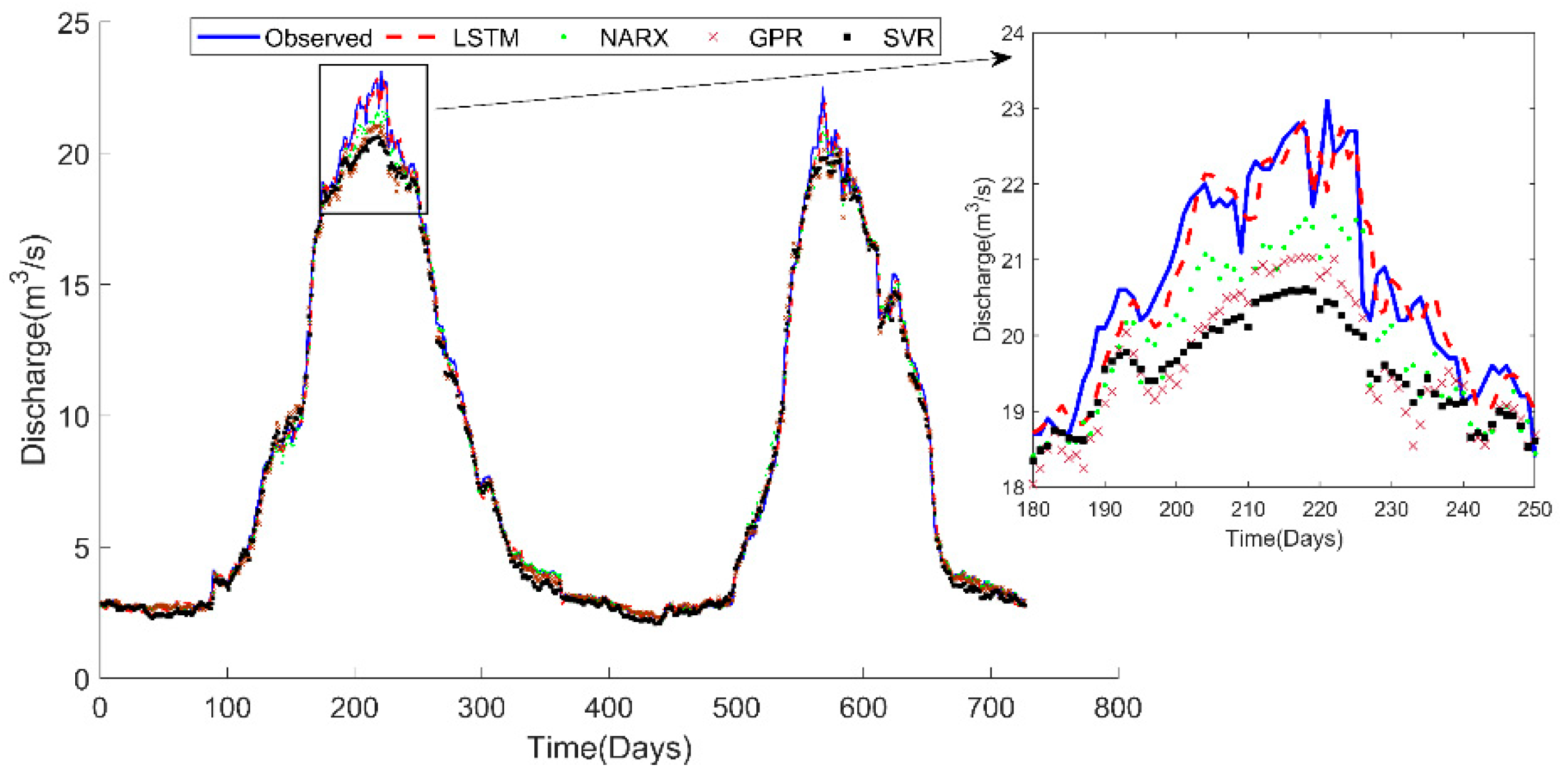
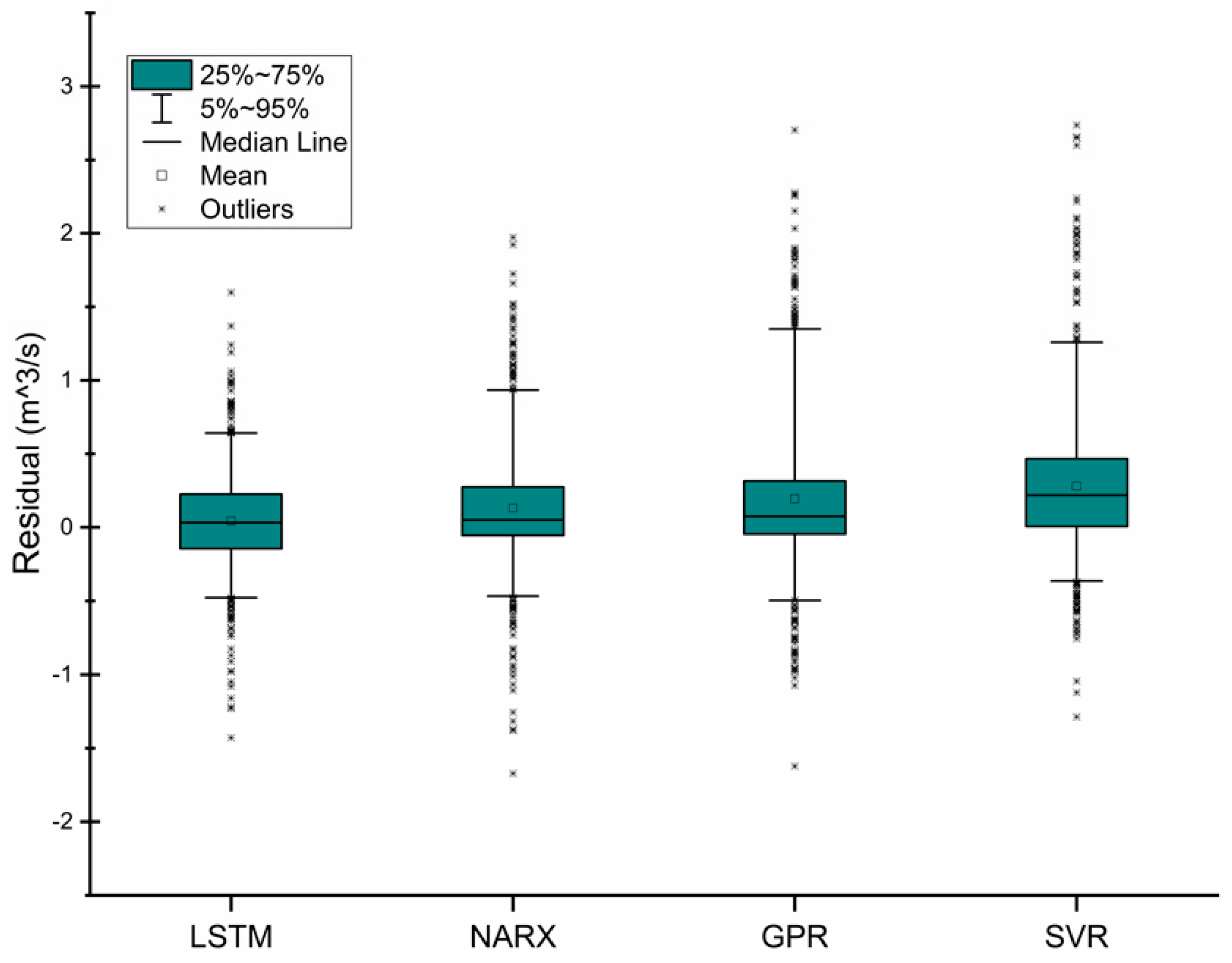
The qualitative assessment of the models is done by visual comparison. From Figure 6, it is observed that the performance of all four models is comparable for normal flow. However, for peak flows, only the LSTM model showed an accurate prediction. The box plot depicting the median and percentiles (5th, 25th, 75th, and 95th) of residuals of simulated river discharge is shown in Figure 7. For a good model, the mean and median of the residuals should lie near to zero. The mean and median of residuals of the LSTM model are closer to zero than that of other models. In the scatterplot diagram, if the points lie near the diagonal line (1:1 line), the model accurately estimates the river discharge. If the points are above the diagonal line (1:1 line), the model overestimates the actual flow and if points are below the diagonal line, the model underestimates the actual flow. From the scatterplot (Figure 8), it is well noticed that all models predict good for low and medium flows but high flows are underestimated by all models except LSTM. The ability of the LSTM model to predict peak flows accurately makes it suitable for use in engineering projects such as reservoir management, hydropower, irrigation, water supply, as well as early flood warning systems.

3.4. Sensitivity Analysis

As discharge data is highly autocorrelated, antecedent discharge values were used for better prediction results. The sensitivity analysis of models for three input conditions, i.e., all inputs (M1), all inputs without precipitation (M2), and all input without SCA (M3), were carried out. The results of the sensitivity analysis are presented in

Table 6. Performance of machine learning (ML) models with different input combinations during the testing phase, all inputs (M1), all inputs without precipitation (M2), and all input without SCA (M3).

Models	Inputs	KGE’	NSE	R2	MAE	RMSE
LSTM	M1	0.99	0.995	0.997	0.124	0.201
	M2	0.99	0.995	0.997	0.112	0.173
	M3	0.988	0.994	0.997	0.186	0.287
NARX	M1	0.971	0.989	0.995	0.312	0.55
	M2	0.974	0.991	0.996	0.28	0.486
	M3	0.969	0.989	0.995	0.317	0.503
GPR	M1	0.947	0.971	0.99	0.601	0.886
	M2	0.95	0.973	0.99	0.564	0.812
	M3	0.944	0.966	0.987	0.634	0.978
SVR	M1	0.945	0.967	0.987	0.605	0.926
	M2	0.949	0.971	0.99	0.561	0.851
	M3	0.942	0.966	0.986	0.641	0.986

. The performance of LSTM model for M2 (KGE = 99%, RMSE = 0.173) is similar to that of M1 (KGE = 99%, RMSE = 0.201) and better than that of M3 (KGE = 98.8%, RMSE = 0.287). The performance of NARX model for M2 (KGE = 97.4%, RMSE = 0.486) is better than that of M1 (KGE = 97.1%, RMSE = 0.55) and M3 (KGE = 96.9%, RMSE = 0.503). For GPR model, M2 combination (KGE = 95%, RMSE = 0.812) returned the best result followed by M1 (KGE = 94.7%, RMSE = 0.886) and M3 (KGE = 94.4%, RMSE = 0.978) respectively. For SVR model, M2 combination (KGE = 94.9%, RMSE = 0.851) returned the best result followed by M1 (KGE = 94.5%, RMSE = 0.926) and M3 (KGE = 94.2%, RMSE = 0.986) respectively. It is well noticed that for all models, the best result is achieved by the M2 input combination. Similar results were depicted by GT.

4. Discussion

In this study, the model efficiency (in terms of NSE) of LSTM, NARX, GPR, and SVR models were found to be 99.5%, 99.1%, 97.3%, and 97.1%, respectively. In a previous study by Pradhananga et al. [49], a positive degree day TI model employed in the Langtang basin for river discharge prediction achieved model efficiency (in terms of NSE) up to 80%, which is much lower than that of all ML models used in this study. Moreover, the ANN model employed by Uysal et al. [11] for 1 day ahead snowmelt runoff prediction in the Upper Euphrates Basin of Turkey achieved the model efficiency (in terms of NSE) up to 93%, which is also lower than that of ML models used in this study. In the study by Le et al. [17], the LSTM model for rainfall-runoff modeling showed the model efficiency (in terms of NSE) up to 99.2%, which is comparable to the result of LSTM model used in this study.

Kratzert et al. [15] employed a two-layered LSTM whereas Le et al. [17] and Fan et al. [16] used the single-layered LSTM, however, these studies did not evaluate the effect of the number of hidden layers on the predictive power of the LSTM model for runoff modeling. In this study, we compared the performance of the LSTM model for several hidden layers (1, 2, and 3 layers) and noticed that the LSTM layer with one hidden layer performed better than the LSTM model with multiple hidden layers. Similar to this, Kratzert et al. [18] also reported that a single-layered stacked LSTM model performs better than two-layered stacked LSTM. From this result, we realized that a single hidden layer LSTM model is adequate, and deeper LSTM models are not essential for streamflow prediction. In their study, Le et al. [17] used SGD optimizer whereas Fan et al. [16] used Adam optimizer. Both studies did not evaluate the influence of optimizer on model performance. In a study by KC et al. [35], the performance of three optimizers was compared and they found that Nadam optimizer was more accurate than SGD and Adam for plant disease detection. In this study, we compared the performance of seven optimizers (Adam, Nadam, Adamax, Adadelta, Adagrad, SGD, RMSprop) and found that Adamax optimizer is superior to other optimizers for runoff modeling.

Kratzert et al. [15] and Kratzert et al. [18] argued that the LSTM model could mimic snow accumulation and melting process by learning the linkage between precipitation during winter and runoff in spring. In this study, we compared the performance of the LSTM model with different input combinations (see Table 6). It is well noticed that SCA as input gives better snowmelt runoff prediction than precipitation as input. The results achieved by the previous studies [15,18] were good enough but could have been better (in the case of snow-influenced catchments) if they had incorporated snow-related data in the input.

Several studies [39,40] used the LM algorithm for training the NARX model. We compared the performance of LM, BR, and SCG algorithms, and the results showed that the BR algorithm performs better than LM and SCG algorithms. The superiority of the BR algorithm over the LM algorithm was also shown by Guzman et al. [38]. In a study, Alsumaiei [39] employed the NARX model for groundwater level forecasting and the results showed the model efficiency up to 99.3%, which is comparable to the performance of the NARX model in this study.

In most of the studies employing ML models [9,11,15,16,18], inputs were determined on an ad-hoc basis or by trial and error method. Input selection is an important task in the model development process for the DD models, however, it is often neglected. The application of GT during the initial phase of the model development process to determine the appropriate input combination reduced the workload which otherwise would have required several experiments. LSTM models used in rainfall-runoff modeling used precipitation data as a key input [15,16,17,18]. Since precipitation is the prime source of river discharge in those catchments, it is obvious to utilize rainfall as input for modeling in those cases. However, in the Himalayan basins, due to low temperature, precipitation is stored in the form of snow and therefore, does not instantly contribute to total runoff. In a study by Thapa et al. [20], it was found that precipitation and river discharge has no significant correlation whereas SCA and river discharge are significantly correlated in the Langtang basin. From the results of sensitivity analysis, it is clear that the models are sensitive to snow cover than precipitation data in the Himalayan basins, which demonstrates the ability of ML techniques to learn the complex physical linkage between input and output.

Due to the sparsity of ground stations, it is hard to obtain ground truth observation in Himalayan basins. Even if available, the ground truth data are not representative of the whole basin due to high elevation difference, as most of the stations are located at lower elevation zones within the Himalayas. In such cases, remotely sensed SCA and meteorological products are invaluable assets for the water resource modeling. The result of this study proves the applicability of ML models in operational streamflow forecasting using remotely sensed products in the data-scant mountainous basins.

5. Conclusions

In this study, four ML models, including LSTM, NARX, SVR, and GPR models are employed for snowmelt driven streamflow prediction. Langtang basin is one of the snow-glacier dominated basins in the Himalayas, therefore, this study area was chosen for the study. The performance of models is assessed by KGE’, NSE, R², RMSE, and MAE. The SCA extracted from MODIS snow products and remotely sensed meteorological data are utilized as inputs to the models. A suitable input combination was selected based on GT.

The LSTM model (KGE’ = 0.99, RMSE = 0.173) outperformed NARX (KGE’ = 0.974, RMSE = 0.486), GPR (KGE’ = 0.95, RMSE = 0.812), and SVR (KGE’ = 0.949, RMSE = 0.851) models. All four ML models achieved good results in discharge prediction (KGE’ > 0.94). However, NARX, GPR, and SVR models slightly underestimated the high flows. While scrutinizing the potentiality of LSTM architecture in snowmelt-runoff prediction, we found the shallow LSTM model with a single hidden layer performing better than deeper models with multiple hidden layers. Out of seven optimizers tested, Adamax was found to be the most suitable optimizer for this study. The results of the GT and sensitivity analysis revealed that the ML models were more sensitive to SCA than precipitation data in the Langtang basin. Therefore, ML models enriched with snow data are appropriate for river discharge prediction in snow-dominated basins.

This study demonstrates the successful application of the LSTM, NARX, GPR, and SVR models in predicting snowmelt driven streamflow. This approach can be easily replicated on other snow-dominated mountainous basins with diverse characteristics where sufficient past river discharge data are available. This work will be useful for estimating water availability for reservoir management, water supply, irrigation, and hydroelectricity projects in the data-scanty mountainous basins.

References

1. Wester, P.; Mishra, A.; Mukherji, A.; Shrestha, A.B. The Hindu Kush Himalaya Assessment; Wester, P., Mishra, A., Mukherji, A., Shrestha, A.B., Eds.; Springer International Publishing: Cham, Switzerland, 2019; ISBN 978-3-319-92287-4. [Google Scholar]
2. Kumar, M.; Marks, D.; Dozier, J.; Reba, M.; Winstral, A. Evaluation of distributed hydrologic impacts of temperature-index and energy-based snow models. Adv. Water Resour. 2013, 56, 77–89. [Google Scholar] [CrossRef]
3. Griessinger, N.; Schirmer, M.; Helbig, N.; Winstral, A.; Michel, A.; Jonas, T. Implications of observation-enhanced energy-balance snowmelt simulations for runoff modeling of Alpine catchments. Adv. Water Resour. 2019, 133, 103410. [Google Scholar] [CrossRef]
4. Ohmura, A. Physical Basis for the Temperature-Based Melt-Index Method. J. Appl. Meteorol. 2001, 40, 753–761. [Google Scholar] [CrossRef]
5. Massmann, C. Modelling Snowmelt in Ungauged Catchments. Water 2019, 11, 301. [Google Scholar] [CrossRef] [Green Version]
6. Martinec, J.; Rango, A. Parameter values for snowmelt runoff modelling. J. Hydrol. 1986, 84, 197–219. [Google Scholar] [CrossRef]
7. ASCE Artificial Neural Networks in Hydrology. I: Preliminary Concepts. J. Hydrol. Eng. 2000, 5, 115–123. [Google Scholar] [CrossRef]
8. ASCE Artificial Neural Networks in Hydrology. II: Hydrologic Applications. J. Hydrol. Eng. 2000, 5, 124–137. [Google Scholar] [CrossRef]
9. Callegari, M.; Mazzoli, P.; de Gregorio, L.; Notarnicola, C.; Pasolli, L.; Petitta, M.; Pistocchi, A. Seasonal River Discharge Forecasting Using Support Vector Regression: A Case Study in the Italian Alps. Water 2015, 7, 2494–2515. [Google Scholar] [CrossRef] [Green Version]
10. De Gregorio, L.; Callegari, M.; Mazzoli, P.; Bagli, S.; Broccoli, D.; Pistocchi, A.; Notarnicola, C. Operational River Discharge Forecasting with Support Vector Regression Technique Applied to Alpine Catchments: Results, Advantages, Limits and Lesson Learned. Water Resour. Manag. 2018, 32, 229–242. [Google Scholar] [CrossRef]
11. Uysal, G.; Şensoy, A.; Şorman, A.A. Improving daily streamflow forecasts in mountainous Upper Euphrates basin by multi-layer perceptron model with satellite snow products. J. Hydrol. 2016, 543, 630–650. [Google Scholar] [CrossRef]
12. Martinec, J. Snowmelt—Runoff model for stream flow forecasts. Hydrol. Res. 1975, 6, 145–154. [Google Scholar] [CrossRef]
13. Nagesh Kumar, D.; Srinivasa Raju, K.; Sathish, T. River Flow Forecasting using Recurrent Neural Networks. Water Resour. Manag. 2004, 18, 143–161. [Google Scholar] [CrossRef]
14. Hochreiter, S.; Schmidhuber, J. Long Short-Term Memory. Neural Comput. 1997, 9, 1735–1780. [Google Scholar] [CrossRef] [PubMed]
15. Kratzert, F.; Klotz, D.; Brenner, C.; Schulz, K.; Herrnegger, M. Rainfall—Runoff modelling using Long Short-Term Memory (LSTM) networks. Hydrol. Earth Syst. Sci. 2018, 22, 6005–6022. [Google Scholar] [CrossRef] [Green Version]
16. Fan, H.; Jiang, M.; Xu, L.; Zhu, H.; Cheng, J.; Jiang, J. Comparison of Long Short Term Memory Networks and the Hydrological Model in Runoff Simulation. Water 2020, 12, 175. [Google Scholar] [CrossRef] [Green Version]
17. Le, X.-H.; Ho, H.V.; Lee, G.; Jung, S. Application of Long Short-Term Memory (LSTM) Neural Network for Flood Forecasting. Water 2019, 11, 1387. [Google Scholar] [CrossRef] [Green Version]
18. Kratzert, F.; Klotz, D.; Shalev, G.; Klambauer, G.; Hochreiter, S.; Nearing, G. Towards Learning Universal, Regional, and Local Hydrological Behaviors via Machine-Learning Applied to Large-Sample Datasets. arXiv 2019, arXiv:1907.0845623, 5089–5110. [Google Scholar] [CrossRef] [Green Version]
19. Kirkham, J.D.; Koch, I.; Saloranta, T.M.; Litt, M.; Stigter, E.E.; Møen, K.; Thapa, A.; Melvold, K.; Immerzeel, W.W. Near real-time measurement of snow water equivalent in the Nepal Himalayas. Front. Earth Sci. 2019, 7, 1–18. [Google Scholar] [CrossRef] [Green Version]
20. Thapa, S.; Li, B.; Fu, D.; Shi, X.; Tang, B.; Qi, H.; Wang, K. Trend analysis of climatic variables and their relation to snow cover and water availability in the Central Himalayas: A case study of Langtang Basin, Nepal. Theor. Appl. Climatol. 2020. [Google Scholar] [CrossRef]
21. RGI Consortium. Randolph Glacier Inventory—A Dataset of Global Glacier Outlines: Version 6.0; GLIMS Technical Report: Boulder, CO, USA, 2017. [Google Scholar] [CrossRef]
22. Ragettli, S.; Pellicciotti, F.; Immerzeel, W.W.; Miles, E.S.; Petersen, L.; Heynen, M.; Shea, J.M.; Stumm, D.; Joshi, S.; Shrestha, A. Unraveling the hydrology of a Himalayan catchment through integration of high resolution in situ data and remote sensing with an advanced simulation model. Adv. Water Resour. 2015, 78, 94–111. [Google Scholar] [CrossRef]
23. Yasutomi, N.; Hamada, A.; Yatagai, A. Development of a Long-term Daily Gridded Temperature Dataset and Its Application to Rain/Snow Discrimination of Daily Precipitation. Glob. Environ. Res. 2011, V15N2, 165–172. [Google Scholar]
24. Huffman, G.J.; Bolvin, D.T.; Nelkin, E.J.; Wolff, D.B.; Adler, R.F.; Gu, G.; Hong, Y.; Bowman, K.P.; Stocker, E.F. The TRMM Multisatellite Precipitation Analysis (TMPA): Quasi-Global, Multiyear, Combined-Sensor Precipitation Estimates at Fine Scales. J. Hydrometeorol. 2007, 8, 38–55. [Google Scholar] [CrossRef]
25. Immerzeel, W.W.; Droogers, P.; de Jong, S.M.; Bierkens, M.F.P. Remote Sensing of Environment Large-scale monitoring of snow cover and runoff simulation in Himalayan river basins using remote sensing. Remote Sens. Environ. 2009, 113, 40–49. [Google Scholar] [CrossRef]
26. NASA—National Aeronautics and Space Administration, TRMM. Available online: https://pmm.nasa.gov/data-access/downloads/trmm (accessed on 9 September 2019).
27. Hall, D.K.; Riggs, G.A. MODIS/Terra Snow Cover 8-Day L3 Global 500 m SIN Grid, Version 6; NASA NSIDC DAAC: Boulder, CO, USA, 2016; Available online: https://nsidc.org/data/mod10a2 (accessed on 29 August 2018). [CrossRef]
28. Stigter, E.E.M.; Wanders, N.; Saloranta, T.M.; Shea, J.M.; Bierkens, M.F.P.P.; Immerzeel, W.W. Assimilation of snow cover and snow depth into a snow model to estimate snow water equivalent and snowmelt runoff in a Himalayan catchment. Cryosphere 2017, 11, 1647–1664. [Google Scholar] [CrossRef] [Green Version]
29. Hall, D.K.; Riggs, G.A.; Salomonson, V.V.; Digirolamo, N.E.; Bayr, K.J. MODIS snow-cover products. Remote Sens. Environ. 2002, 83, 181–194. [Google Scholar] [CrossRef] [Green Version]
30. NASA/METI/AIST/Japan Spacesystems, and U.S./Japan ASTER Science Team. ASTER Global Digital Elevation. Modeldistributed by NASA EOSDIS Land Processes DAAC; 2009. Available online: https://lpdaac.usgs.gov (accessed on 4 April 2018). [CrossRef]
31. Maier, H.R.; Jain, A.; Dandy, G.C.; Sudheer, K.P. Methods used for the development of neural networks for the prediction of water resource variables in river systems: Current status and future directions. Environ. Model. Softw. 2010, 25, 891–909. [Google Scholar] [CrossRef]
32. Stefánsson, A.; Končar, N.; Jones, A.J. A note on the gamma test. Neural Comput. Appl. 1997, 5, 131–133. [Google Scholar] [CrossRef]
33. Durrant, P.J. WinGamma: A Non-Linear Data Analysis and Modelling Tool with Applications to Flood Prediction; Cardiff University: Wales, UK, 2001. [Google Scholar]
34. Chollet, F. Keras. Available online: https://keras.io (accessed on 14 October 2019).
35. KC, K.; Yin, Z.; Wu, M.; Wu, Z. Depthwise separable convolution architectures for plant disease classification. Comput. Electron. Agric. 2019, 165, 104948. [Google Scholar] [CrossRef]
36. Srivastava, N.; Hinton, G.; Krizhevsky, A.; Sutskever, I.; Salakhutdinov, R. Dropout: A Simple Way to Prevent Neural Networks from Overfitting. J. Mach. Learn. Res. 2014, 15, 1929–1958. [Google Scholar] [CrossRef]
37. Lin, T.; Horne, B.G.; Tino, P.; Giles, C.L. Learning long-term dependencies in NARX recurrent neural networks. IEEE Trans. Neural Netw. 1996, 7, 1329–1338. [Google Scholar] [CrossRef] [Green Version]
38. Guzman, S.M.; Paz, J.O.; Tagert, M.L.M. The Use of NARX Neural Networks to Forecast Daily Groundwater Levels. Water Resour. Manag. 2017, 31, 1591–1603. [Google Scholar] [CrossRef]
39. Alsumaiei, A.A. A Nonlinear Autoregressive Modeling Approach for Forecasting Groundwater Level Fluctuation in Urban Aquifers. Water 2020, 12, 820. [Google Scholar] [CrossRef] [Green Version]
40. Banihabib, M.E.; Bandari, R.; Peralta, R.C. Auto-Regressive Neural-Network Models for Long Lead-Time Forecasting of Daily Flow. Water Resour. Manag. 2019, 33, 159–172. [Google Scholar] [CrossRef]
41. Vapnik, V.N. The Nature of Statistical Learning Theory; Springer New York: New York, NY, USA, 1995; Volume 66, ISBN 978-1-4757-2442-4. [Google Scholar]
42. Dibike, Y.B.; Velickov, S.; Solomatine, D.; Abbott, M.B. Model Induction with Support Vector Machines: Introduction and Applications. J. Comput. Civ. Eng. 2001, 15, 208–216. [Google Scholar] [CrossRef]
43. Rasmussen, C.E.; Williams, C.K.I. Gaussian Processes for Machine Learning; The MIT Press: Cambridge, MA, USA, 2006. [Google Scholar]
44. Wang, J.; Hu, J. A robust combination approach for short-term wind speed forecasting and analysis—Combination of the ARIMA (Autoregressive Integrated Moving Average), ELM (Extreme Learning Machine), SVM (Support Vector Machine) and LSSVM (Least Square SVM) forecasts using a GPR (Gaussian process regression) model. Energy 2015, 93, 41–56. [Google Scholar] [CrossRef]
45. Kling, H.; Fuchs, M.; Paulin, M. Runoff conditions in the upper Danube basin under an ensemble of climate change scenarios. J. Hydrol. 2012, 424, 264–277. [Google Scholar] [CrossRef]
46. Nash, J.E.; Sutcliffe, J.V. River flow forecasting through conceptual models part I—A discussion of principles. J. Hydrol. 1970, 10, 282–290. [Google Scholar] [CrossRef]
47. Bengio, Y. Practical recommendations for gradient-based training of deep architectures. In Neural Networks: Tricks of the Trade; Springer: Cham, Switzerland, 2012; pp. 1–33. [Google Scholar]
48. Kingma, D.P.; Ba, J. Adam: A Method for Stochastic Optimization. arXiv 2014, arXiv:1412.6980. [Google Scholar]
49. Pradhananga, N.S.; Kayastha, R.B.; Bhattarai, B.C.; Adhikari, T.R.; Pradhan, S.C.; Devkota, L.P.; Shrestha, A.B.; Mool, P.K. Estimation of discharge from Langtang River basin, Rasuwa, Nepal, using a glacio-hydrological model. Ann. Glaciol. 2014, 55, 223–230. [Google Scholar] [CrossRef] [Green Version]
Figure 1. Map of the study area.
Water 12 01734 g001
Figure 2. A typical LSTM cell, where σ denotes sigmoidal function, tanh denotes a hyperbolic tangent function, f stands for forget gate, i denotes input gate, o denotes output gate, h is the hidden state, c denotes cell state, x is input vector at time step t.
Water 12 01734 g002
Figure 3. A typical NARX structure (a) parallel (b) series-parallel.
Water 12 01734 g003
Figure 4. Monthly variation of snow cover area (SCA) in Langtang basin during the research period (2002–2012).
Water 12 01734 g004
Figure 5. Performance of LSTM model in terms of mean absolute error (MAE) and root mean square error (RMSE) for (a) number of LSTM layers (b) number of hidden units (c) Optimizers.
Water 12 01734 g005
Figure 6. Comparison of observed and simulated flows.
Water 12 01734 g006
Figure 7. Boxplot of residuals.
Water 12 01734 g007
Figure 8. Scatter plot of predicted flow with observed flow (a) LSTM model (b) NARX model (c) GPR model (d) SVR model. The solid line is the 1:1 line.
Water 12 01734 g008