Species-Richness Responses to Water-Withdrawal Scenarios and Minimum Flow Levels: Evaluating Presumptive Standards in the Tennessee and Cumberland River Basins

Abstract

Water-resource managers are challenged to balance growing water demand with protecting aquatic ecosystems and biodiversity. Management decisions can benefit from improved understanding of water-withdrawal impacts on hydrologic regimes and ecological assemblages. This study used ecological limit functions for fish groups within the Tennessee and Cumberland River basins to predict species richness responses under simulated constant-rate (CR) and percent-of-flow (POF) withdrawals and for different minimum flow level protections. Streamflow characteristics (SFC) and richness were generally less sensitive to POF withdrawals than CR withdrawals among sites, fish groups, and ecoregions. Species richness generally declined with increasing withdrawals, but responses were variable depending on site-specific departures of SFCs from reference conditions, drainage area, fish group, ecoregion, and minimum flow level. Under POF withdrawals, 10% and 20% daily flow reductions often resulted in loss of <1 species and/or ≤5% richness among fish groups. Median ecological withdrawal thresholds ranged from 3.5–31% for POF withdrawals and from 0.01–0.92 m³/s for CR withdrawals across fish groups and ecoregions. Application of minimum flow level cutoffs often resulted in damping effects on SFC and richness responses, indicating that protection of low streamflows may mitigate hydrologic alteration and fish species richness loss related to water withdrawals. Site-specific and regionally summarized responses of flow regimes and fish assemblages under alternative withdrawal strategies in this study may be useful in informing water-management decisions regarding streamflow allocation and maintaining ecological flows.

1. Introduction

The natural flow regime is considered a master variable in determining lotic ecosystem processes [1]. It is well documented that alterations of streamflow regimes pose significant threats to riverine ecosystems and biodiversity worldwide [2,3,4,5,6]. Many studies have shown that aquatic communities can be negatively impacted by alteration of the magnitude, timing, and/or duration of flows to which they are adapted [2,4,5,6,7,8]. Water withdrawals for domestic, agricultural, and industrial purposes can directly reduce streamflow quantity and disrupt the natural timing and variability of flows [9]. With increasing human population and intensifying land-use practices, global water withdrawals have already increased dramatically over the past 50 years [10] and are expected to continue [11].

Effects of streamflow alteration on fish have been shown to be variable and context dependent but can have significant negative impacts on fish growth, reproduction, and survival, and ultimately community composition and diversity [5,8]. For example, altered streamflow variability has been associated with a loss of species richness [5], particularly among riffle-dwelling species [12,13], and reductions in streamflow via water withdrawals have been shown to impact the composition and structure of fish assemblages, specifically the occurrence and proportion of fluvial-dependent species [14,15].

As the global water demand continues to intensify, water-resource managers face increasing challenges to satisfy societal water needs while also protecting ecosystem flow requirements and biodiversity [6,16,17,18]. In the past several decades, much effort has been given to developing statistical and methodological frameworks to describe and quantify flow-ecology relationships to better inform resource managers and set conservation targets [3,18,19,20,21,22,23]. Despite increasing awareness of the importance of flow-ecology relationships [16,18,24] and continuing efforts to translate these relationships into decision support systems, the integration and implementation of ecological-flows management guidelines are continuing challenges at local and regional scales [25,26,27].

Resource managers seek accessible and easily implemented guidelines on water-withdrawal practices [18]. For example, minimum flow requirements and protection of minimum flow levels (MFL), which prohibit withdrawals when streamflow falls below specified critical levels, were some of the earliest ecological flow management strategies and are still commonly utilized [28]. However, it is well recognized that employment of MFLs alone are often insufficient to protect stream integrity across a range of hydrologic conditions [1,18,26,29]. Constant-rate (CR) withdrawal strategies are generally fixed withdrawal rates and are not related to changes in ambient flows. CR withdrawals are commonly used, proposed, or permitted for various surface and groundwater-withdrawal purposes based on the amount of water needed (i.e., consumer demand), the overall withdrawal capacity (i.e., supply and pumping capacity) of a facility, or basic rules-of-thumb, rather than on empirical, evidence-based ecological-flow relationships or dynamic environment and flow conditions. The potential for hydrologic and ecologic impacts of CR withdrawals can be quite high because CR withdrawals can strongly affect the streamflow regime by altering the natural (or baseline) variability of flows, particularly aspects of low flow. On the other hand, variable-rate water-withdrawal strategies based, for example, on set percentages of the natural or baseline flow regime (i.e., percentage-of-flow, POF) are increasingly recognized as attractive water-management strategies because they exert proportional withdrawals on the underlying flow regime and thereby are better suited to preserving natural variability of flows across the entire hydrograph [29,30]. More recently, presumptive POF water-withdrawal standards have been proposed at 10–20% of daily streamflow [30] which, in theory, inherently provide ecological protection. POF withdrawals and presumptive standards are conceptually simple strategies that can be easily adopted by water-resource managers, but implementation of POF withdrawals requires accurate streamflow measurements on a frequent time step (e.g., daily), and the ability to adjust withdrawal rates in real time. Although the vast majority of streams are ungauged, discrete or instantaneous streamflow can be measured using relatively simple methods [31], and prediction of steamflow at ungauged locations may be possible using basin-area/runoff models [32].

Possible disconnects exist between the cost, time, and amount of information needed to establish sound evidenced-based environmental flow requirements versus the type and urgency of information often sought by resource managers. These mismatches can prohibit or slow the practical implementation of flow-ecology guidelines, particularly under contentious social, political, and economic contexts [19,21,26]. In the meantime, water-resource managers and regulators are commonly left to make decisions based on generalized rules-of-thumb and experience rather than evidence-based approaches [18,21,26,33].

Water-management decisions associated with permitting and allocation of water withdrawals can benefit from a better understanding of how different streamflow-withdrawal strategies impact ecological communities and the establishment of evidence-based guidelines to balance water withdrawals and protection of ecological assemblages [18,27,30]. Specifically, current understanding is limited regarding the range of potential ecological responses along a gradient of hydrologic alteration scenarios (i.e., so-called “top-down” approach; [19]) using plausible water-management strategies (e.g., water-withdrawal rates and MFL protections). Additionally, there is little consensus regarding what might be considered ‘acceptable’ limits of ecological change (e.g., species loss) or biological condition with which to establish potential ecological-flow thresholds [21,22,34,35]. Despite the growing number of ecological-flow studies investigating ecological responses in relation to various types of flow alteration (e.g., related to climate change, impoundments, withdrawals, and land-use changes) [5,17,26,34,36], few have explored these relationships in an incremental fashion across relatively long alteration gradients or set out to identify ecological or hydrologic thresholds.

This study expands on a series of previously developed hydrologic and ecological relationships within the Cumberland River and Tennessee River basins [37,38,39,40,41]. We used published ecological-limit functions (ELFs) [39,41] for fish groups within Blue Ridge (BR), Ridge and Valley (RV), Interior Plateau (IP), and Cumberland Plateau (CP) Level III ecoregions [42] to model incremental changes in streamflow characteristics (SFCs) and species richness responses along gradients of simulated withdrawal scenarios. We ran these simulations using simplified CR and POF withdrawal strategies and different MFL protections. The primary objectives of this study were to (1) simulate water withdrawals and characterize potential hydrologic and ecological impacts of CR and POF scenarios and (2) identify potential withdrawal thresholds below which conservative levels of species richness loss may be minimized.

We investigated the following general hypotheses related to hydrologic and ecological impacts of CR compared to POF withdrawals: (1) SFCs should be less sensitive to POF withdrawal scenarios than to CR withdrawals, particularly SFCs associated with flow ratios, frequency, variability, and timing of flows; (2) resulting predicted fish species richness should generally decrease with increased water withdrawals regardless of CR or POF withdrawals; and (3) application of MFLs should generally dampen patterns of change of SFCs, species richness, and withdrawal threshold responses regardless of CR or POF withdrawals.

2. Materials and Methods

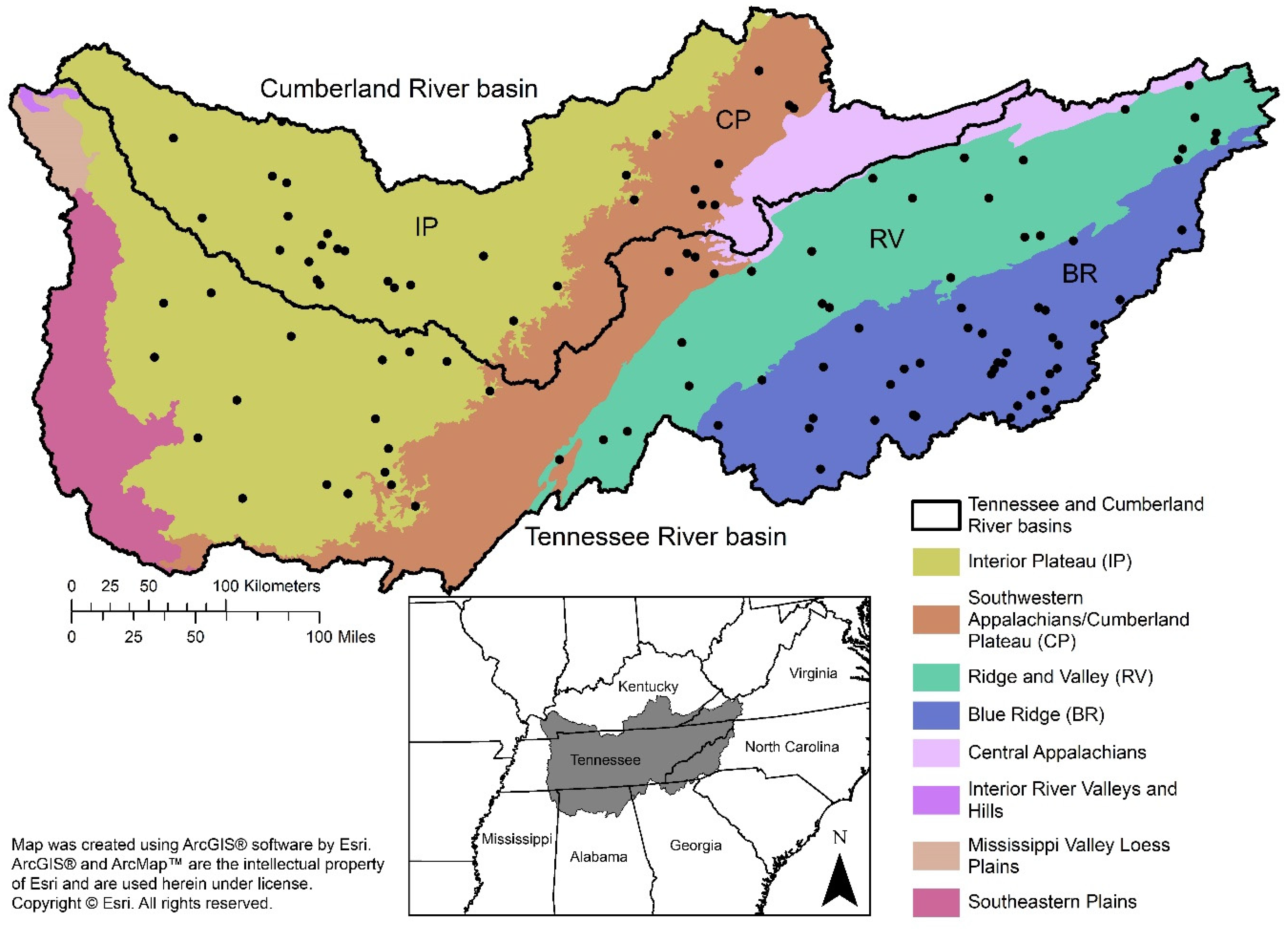
Data analyses and prediction of ecological effects of water-withdrawal scenarios were performed using flow-ecology relationships (i.e., ELFs) that were developed in a series of previously published studies conducted on stream sites within the Tennessee and Cumberland River basins [37,38,39,41]. In [37], a large suite of SFCs were statistically related to metrics of fish diversity at select free-flowing gauged stream sites and a subset of ecologically significant SFCs were identified for the BR, RV, CP, and IP ecoregions (see

Table 1. Definitions of streamflow characteristic (SFC) used in ecological limit functions and the respective ecoregion(s) where they were found to be statistically significant; modified from [39].

Flow Category	Streamflow Characteristic (SFC)	Definition (Units)	Eco-Region
Magnitude	MA41: mean annual runoff	Annual mean streamflow divided by the drainage area (ft3s−1mi−2)	RV, CP
	AMH10: maximum October streamflow	Maximum October flow across period of record divided by watershed area (ft3s−1mi−2)	BR, CP, IP
	LRA7: rate of streamflow recession	Log of the median change in log of flow for days that the change is negative across the entire flow record (flow units per day)	IP
Ratio	LDH13: average 30-day maximum	Log of the average over period of record of annual maximum 30-day moving average flows divided by median for entire record	CP
	ML20: base flow	Divide daily flow record into 5-day blocks. Assign minimum (min.) flow for the block as a base flow if 90% of that min. flow is less than the min. flows for blocks on either side; otherwise, set to zero. Fill in zero values using linear interpolation. Compute total flow and total base flow for entire record. ML20 is total flow: total base flow (ratio)	CP
	TA1: constancy	Measure the stability of flow regimes by dividing daily flows into predetermined flow classes	RV, CP, IP
Frequency	FH6: frequency of moderate flooding	Average number of high-flow events per year ≥ 3 times the median annual flow for the period of record (number per year)	IP
Variability	LDL6: variability of annual minimum daily average streamflow	Log of the standard deviation for the annual minimum daily average streamflow. Multiply by 100 and divide by the mean streamflow for the period (%)	CP
	LDH16: variability in high-pulse duration	Log of the standard deviation for the yearly average high-flow pulse durations (daily flow > 75th percentile) (%)	RV
	FL2: variability in low-pulse count	Coefficient of variation for the number of annual occurrences of daily flows < 25th percentile	RV
Timing	TL1: annual min. flow	Date of annual mininum (min.) flow occurrence (Julian day)	CP, IP

).

Hydrological reference profiles (i.e., interquartile ranges; IQR) of SFCs were then defined for reference streams within BR, RV, and IP [38,39] and CP [41]. Finally, ELFs were developed using quantile regression that described the upper limits (≥85th quantile) of species richness responses among different fish groups as a function of the hydrologic departure from reference of SFC(s) among streams within BR, RV, and IP [39] and CP [41].

2.1. Study Area

The geographic scope of this study includes the Tennessee and Cumberland River basins, which together drain approximately 150,000 km² in Tennessee, Virginia, Georgia, Alabama, Mississippi, and Kentucky in the USA (Figure 1). Population growth, intensification of land-use practices, and growing demand for surface water and groundwater throughout this region pose increasing risks for hydrologic alteration and degradation of water quality [10]. Further, with more than 250 species of fish, 115 crayfish, 141 freshwater mussels, and 160 aquatic snails, including more than 100 taxa identified as being at risk, the Tennessee and Cumberland River basins collectively represent a major concentration of North American freshwater biodiversity and one of the most diverse temperate freshwater systems in the world [43,44].

The Tennessee and Cumberland River basins transect multiple Level III ecoregions [42], including the Blue Ridge, Ridge and Valley, Interior Plateau, and Southwestern Appalachians. The Southwestern Appalachians Level III ecoregion generally corresponds with the ‘Cumberland Plateau’ physiographic section [45] (Figure 1). In order to maintain consistency with adjacent ecoregion boundaries used in [39], as well as maintain consistency of ecoregion terminology used in [41], we refer to the Southwestern Appalachians Level III ecoregion as the Cumberland Plateau (CP) throughout this paper.

2.2. Site Selection

U.S. Geological Survey (USGS) streamgauge sites within the Cumberland River basin (4-digit hydrological unit code, HUC4: 0513) and Tennessee River basin (HUC4s: 0601, 0602, 0603, 0604) and within BR, RV, CP, and IP Level III ecoregions [42] were initially screened for inclusion. USGS sites with drainage areas ranging from 26–3890 km² and with daily streamflow records for a minimum of 15 complete water years (following recommendations in [46]) between 1975 and 2016 were retained for this study. Prior or existing hydrologic alteration was not considered for site selection. Web-based satellite imagery was used to identify water-control structures and streamgauge sites within close downstream proximity were excluded from analysis. Sites located outside the geographic extent of stream sites used in prior model development [38,39,41] were also excluded. For example, development of ELFs for CP streams was based on sites and datasets from the northern portion of the ecoregion [41] and thus USGS streamgauge sites from the southern portion of CP were not used in this analysis (see Figure 1). Out of 641 USGS daily streamgauge sites across the HUC4s, a total of 112 USGS sites were retained across the four ecoregions: IP, 41 sites; CP, 11 sites; RV, 25 sites; and BR, 35 sites (Figure 1). To assess potential patterns associated with stream size, sites were categorized according to drainage area: 25–130 km², 130–260 km², 260–780 km², 780–1300 km², 1300–2600 km², and 2600–3890 km².

2.3. Water-Withdrawl Models

Mean daily streamflow data for each of the retained stream sites were accessed from USGS National Water Information System (NWIS) database [47]. Hydrologic data sets were queried using the “dataRetrieval” package [48] and R statistical software [49]. For each site, water-withdrawal scenarios were simulated from these observed (baseline) streamflow datasets. For this study, simulated water withdrawals were assumed to be the only source of streamflow alteration during the period of record for each site and previous or existing alterations (e.g., upstream withdrawals or effluent discharges) were assumed to be negligible.

2.3.1. Constant-Rate (CR) Withdrawals

The CR withdrawal model simulated the application of a constant-rate of water withdrawal across the entire period of record for each site, regardless of variability in ambient daily streamflow. A series of incremental CR withdrawal scenarios, ranging from 0.003 to 0.028 m³/s by 0.003 m³/s increments and 0.028 to 1.416 m³/s by 0.028 m³/s increments, were individually simulated for each site by subtracting simulated withdrawals from the baseline daily streamflow data set. CR withdrawal scenario increments were initially constructed using cubic feet per second (ft³/s) units and then later converted to metric units. A total of 60 CR withdrawal scenarios (i.e., hydrographs), including the baseline dataset, were simulated for each site and for each of 4 MFLs (detailed in Section 2.3.3). Because the amount of daily withdrawal was held constant during high or low flows, CR withdrawals were anticipated to disproportionately affect periods of low streamflow (Figure 2a).

2.3.2. Percent-of-Flow (POF) Withdrawals

The POF model simulated the withdrawal of set percentages of measured daily streamflow for each site, ranging from 1% to 40% daily streamflow withdrawal at 1% increments (i.e., total of 41 POF withdrawal scenarios, including the baseline data set, for each site and for each MFL). For the POF model, the absolute amount of simulated water withdrawal during high flows is greater than during low-flow periods, although the relative proportion of withdrawals is held constant. In general, hydrographs simulated under incremental POF withdrawal scenarios were anticipated to be susceptible to an overall reduction in streamflow magnitude but, in contrast to CR withdrawals, POF scenarios should theoretically better preserve aspects of timing, ratios, and variability of streamflows in relation to the baseline hydrograph for each site (Figure 2b). To prevent simulation of unrealistic daily withdrawal rates during higher flows (i.e., withdrawals beyond the pumping capacity of most facilities), a maximum instantaneous withdrawal limit was set at 1.41 m³/s, which was approximately the 99th percentile of all reported annual mean monthly withdrawals from permitted water-withdrawal facilities across Tennessee during 2010 [50].

2.3.3. Minimum Flow Level (MFL) Protection

Four MFLs were applied to each incremental withdrawal scenario to investigate the potential effects of low-flow protections on simulated CR and POF withdrawals. MFLs were defined as set daily streamflow values below which additional withdrawal was prohibited. MFL scenarios were applied at 0%, 5%, 10%, and 30% (MFL0, MFL5, MFL10, MFL30, respectively) of the mean annual daily flow calculated for the period of record of each site. MFL0 represents the absence of minimum-flow protection such that streamflow was allowed to be withdrawn to 0 m³/s under certain circumstances (see Figure 2a). Withdrawal scenarios using MFL0 were used as the basis for comparison of the hydrologic and ecologic effects of simulated water withdrawals. Importantly, for both CR and POF models, water withdrawals were treated as ‘consumptive’, meaning that water returns (i.e., effluent discharges) from upstream withdrawals were not accounted for.

2.4. Data Processing and Analyses

2.4.1. Calculation of SFCs

Prior to simulation of water withdrawals, baseline daily streamflow datasets were formatted for compatibility with the EflowStats R package [51]. The core functions of EflowStats calculate a series of SFCs from a daily streamflow data set, using water years defined as 365 daily flow values beginning on 1 October of one year and ending on 30 September of the following year(s). Gaps in the daily hydrograph were identified and incomplete water years were removed. The final baseline data set for each site consisted of either one continuous or several non-continuous periods that together totaled a minimum of 15 complete water years.

For each site, SFCs were calculated for each data period for 1) the baseline (observed) hydrograph and 2) hydrographs simulated under each incremental withdrawal scenario using CR and POF withdrawal models. For sites with multiple data periods (i.e., sites with gaps in the streamflow record), average SFC values were taken across periods for each withdrawal scenario. For example, for a site with two data periods—a 5-year period and a 10-year period—SFCs were calculated for each period and a weighted average was calculated using the number of water years as the weighting variable. SFC values for each withdrawal scenario were then transformed to standardized (unitless) values using published mean and standard deviation values of SFCs and formulae previously reported in [38].

2.4.2. SFC Sensitivity

Patterns of changes in standardized SFCs in response to incremental water-withdrawal scenarios were visually assessed by plotting SFC values for each site across withdrawal scenarios and for each MFL in relation to reference IQRs of SFCs for each ecoregion (e.g., Figure 3a and Figures S1–S8). The mean sensitivity of each SFC under CR and POF withdrawals was determined by calculating the mean absolute change in SFC values across all incremental withdrawal scenarios relative to the baseline hydrograph for each site and then taking the mean across all sites for each ecoregion. SFCs were considered generally sensitive to water withdrawals if the mean sensitivity for MFL0 was greater than 0. The presence of damping effects of MFLs was indicated by relatively lower mean sensitivity of SFCs at MFL5, MFL10, and/or MFL30 in relation to MFL0. The relative magnitudes of change in mean sensitivity as well as the appearance of ‘dampened’ SFC withdrawal responses based on MFLs (i.e., decreasing slope of site-specific responses with increasing MFLs; see Figure 3a) were used to compare the relative strength and consistency of damping effects for some SFCs among ecoregions as well as generally between CR and POF withdrawals. For example, SFCs that exhibited relatively small decreases in mean sensitivity and subtle or indistinguishable responses to MFLs were considered to have relatively weak damping effects. Damping effects on SFCs were considered absent if an SFC showed no change in mean sensitivity across MFLs or if mean sensitivities of MFL5, MFL10, and MFL30 were each greater than MFL0 (i.e., considered an anomalous or unpredicted increase in sensitivity due to application of MFLs).

2.4.3. Departure from Reference

Departures of SFCs from hydrologic reference conditions were quantified for each incremental withdrawal scenario for each site by calculating the absolute difference of standardized SFC values from reference IQRs of SFCs for each ecoregion. For example, calculated SFC values for each withdrawal scenario that were within the reference IQR (i.e., >25th and <75th percentile values) (e.g., Figure 3a) received a hydrologic departure value of 0, whereas values outside of the IQR (i.e., <25th or >75th percentiles) received a departure value > 0. We note that by using absolute departures values, neither the initial relative position nor the direction of change in departure for each withdrawal scenario in relation to reference IQR are specifically known. Absolute departures of SFCs were then summed across the relevant SFC(s) that defined the ELF for each fish group (Table S1; [39,41]) to arrive at a cumulative hydrologic departure value for each withdrawal scenario for each site for each fish group.

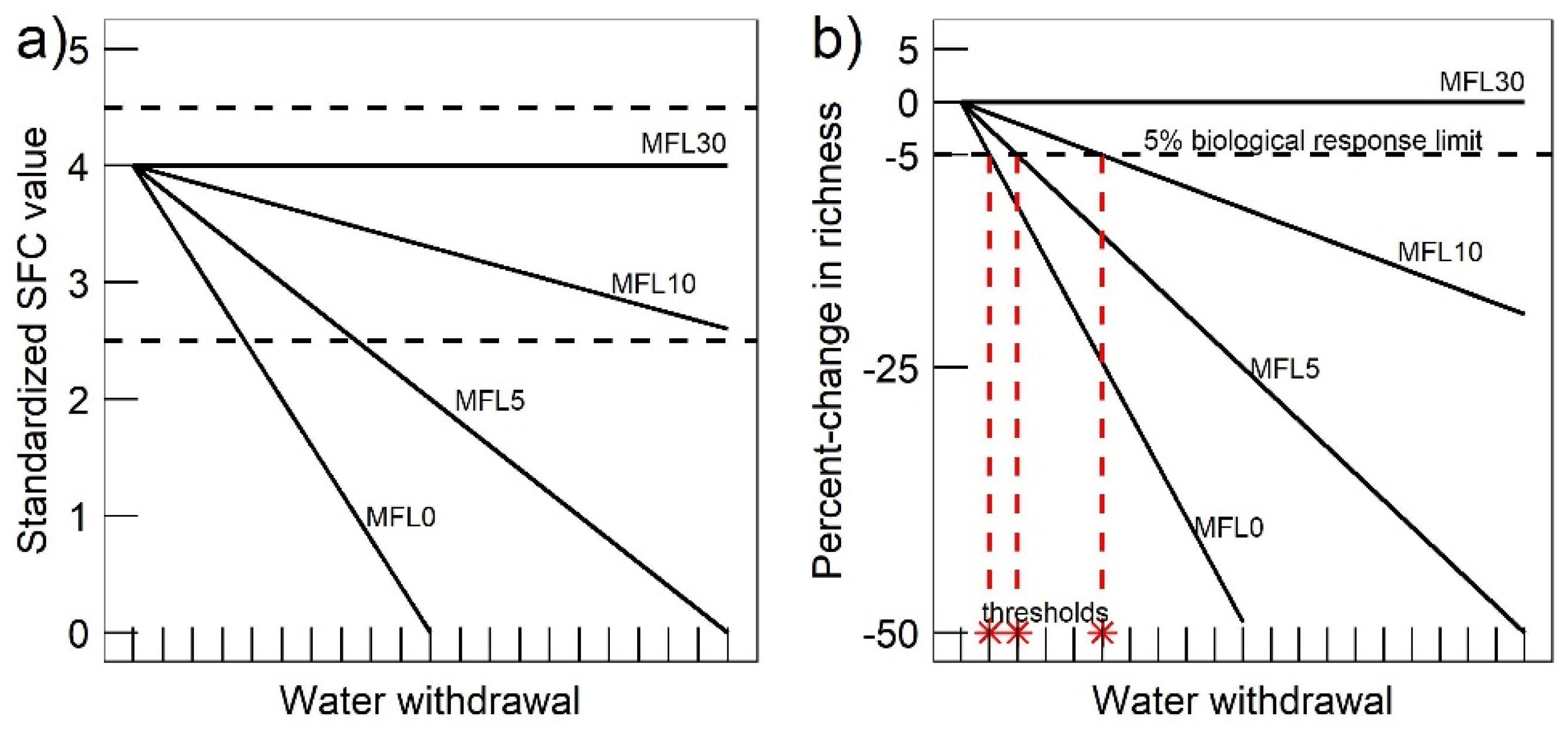
2.4.4. Predicted Species Richness Responses to Withdrawal Scenarios

The ELF for each fish group defines the upper limit (≥85th percentile) of observed fish species richness as a function of the cumulative hydrologic departure of SFCs from reference hydrologic condition [39,41]. Predicted richness under each water-withdrawal scenario, including the original baseline streamflow data set, was calculated for each stream site by solving the following equation for each ELF:

SR = m × x + b

(1)

where SR is predicted species richness, x is cumulative hydrologic departure and m and b are the slope and y-intercept of the ELF for each fish group [39,41] (see Table S1). Because the slope of each ELF is negative (Table S1), cumulative departure values > 0 result in predicted species richness less than the theoretical maximum richness for each fish group (i.e., y-intercept). It is important to note that predicted species richness for any given stream site may increase, decrease, or remain unchanged among withdrawal scenarios depending on the relative change in cumulative departure among relevant SFC(s) between scenarios. For example, predicted species richness will decrease if increasing water withdrawals causes one or more SFC(s) to move farther from the reference condition (i.e., increase in departure). Conversely, predicted richness would increase if departures decreased.

To summarize overall patterns and direction of change in predicted species richness among fish groups, first the mean change in richness was calculated for each withdrawal scenario relative to richness predicted for the baseline hydrologic regime for each site, and then an overall mean was taken across sites for each fish group. Predicted species richness values were also converted to the percent change in richness relative to the richness predicted for the baseline hydrologic regime for each site and plotted to allow more consistent comparison of change in richness among streams and ecoregions with potentially different richness values (e.g., small versus large streams). Negative and positive values represent the predicted relative loss or gain, respectively, of species richness. It is important to note that large positive values of percent change in predicted richness in relation to baseline can result from relatively small increases in predicted species richness among withdrawal scenarios. We recognize that increases in species richness in response to increased water withdrawals are possible under certain circumstances, for example, streams with higher than normal flows (e.g., due to dam release) and/or rivers where reduced velocities and water depths could create additional habitat suitable to more species. However, actual gains in fish species richness are likely to be modest. As such, large gains in predicted richness (absolute or percent change) were considered mathematical artifacts rather than plausible real-world outcomes to increased water withdrawals.

Further, to compare the magnitude of species-richness loss under POF withdrawals with increasingly utilized “presumptive” percent-of-flow standards [30], mean absolute loss and mean percent loss of species richness were calculated across stream sites for 10 and 20 POF withdrawal scenarios for MFL0 for each fish group and ecoregion. Stream sites that did not result in any loss in richness among withdrawal scenarios were excluded from this analysis.

2.4.5. Biological Response Limit and Maximum Withdrawal Thresholds

A 5% loss of species richness (i.e., −5% change relative to richness predicted under baseline hydrologic conditions) was set as an arbitrary biological response limit at which to identify potential withdrawal thresholds for each stream site. Specifically, for any given stream site modeled for each fish group and MFL, an ecological withdrawal threshold (also referred to hereafter as ‘withdrawal threshold’ or simply ‘threshold’) was identified at the maximum incremental water-withdrawal scenario that resulted in less than 5% loss of species richness. Figure 3b illustrates hypothetical examples of monotonic percent changes in species richness along a withdrawal gradient and for different MFLs for a single stream site and identifies different ecological withdrawal thresholds at which richness loss reaches −5%. Damping effects of MFLs on percent change in richness should generally appear as a decreased slope of species richness responses when plotted in relation to MFL0 (e.g., solid lines in Figure 3b), whereas damping effects of MFLs on withdrawal thresholds should appear as (a) higher threshold values with higher MFLs (e.g., asterisks in Figure 3b) or (b) a shift to no threshold in relation to MFL0 (e.g., MFL30 in Figure 3b).

Because species richness varies naturally among streams and because each fish group contains varying subsets of species, using percent loss of predicted species richness to inform a biological response limit—rather than absolute richness values—provides a consistent and scalable metric of biological change across stream sites, fish groups, and ecoregions. A 5% biological response limit is protective of 95% of the relative species richness of each fish group and should buffer against the loss of some sensitive species while still allowing for some water withdrawals to meet human needs. While similar biological response limits have been previously proposed [13,52], there is little consensus (among ecologists, resource managers, citizens, policy makers, or other stakeholders) regarding the degree of change in biological condition (i.e., absolute or percent species-loss) that could/should be tolerated in response to hydrologic alteration [22,34].

Withdrawal thresholds identified under the CR model are reported as daily streamflow withdrawal rates (m³/s) and POF thresholds are reported as percentages of daily streamflow withdrawals (%). Boxplots were used to summarize the distributions and patterns of thresholds among fish groups and by drainage area for each MFL scenario. Median values calculated among all thresholds for each fish group, and overall regional mean withdrawal thresholds calculated across these median values were used to summarize central tendencies among sites, fish groups, and ecoregions. Additionally, the number of sites that reached an ecological withdrawal threshold was calculated for each fish group, and the cumulative number of sites that reached a threshold across all fish groups was summed for each ecoregion. Because each stream site was modeled independently for each fish group, sites that reached a threshold in multiple fish groups were counted more than once.

2.4.6. Model Archive and Bulk Data

A model archive containing detailed R scripts with reproducible procedures as well as bulk data tables containing site-specific results for standardized SFCs, cumulative departures, predicted species richness, percent-change in richness, and withdrawal thresholds for each MFL scenario for both CR and POF withdrawals are available from [53]. Supporting information and large format data summary tables are provided as supplementary tables (Tables S1–S4). Plotted responses among all stream sites for each SFC (Figures S1–S8) and percent-changes in richness (Figures S9–S16) and ecological withdrawal thresholds (Figures S17 and S18) for each fish group MFL and ecoregion are provided as supplementary figures.

3. Results

3.1. Sensitivity of Streamflow Characteristics

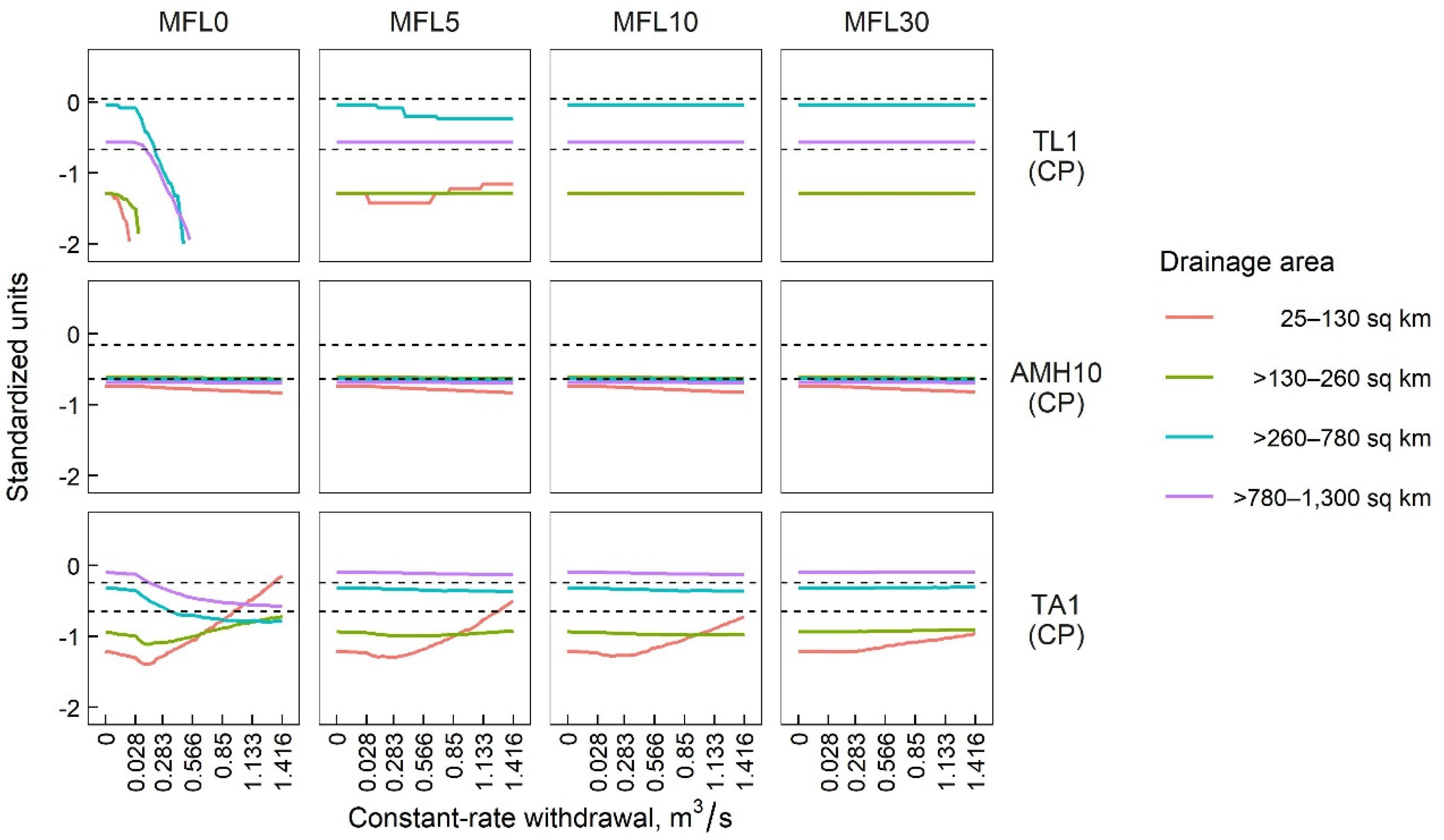
3.1.1. Sensitivity of SFCs to CR Withdrawals

Each SFC showed some sensitivity to CR withdrawals (i.e., mean values greater than 0) for MFL0, although the relative degree of sensitivity (

Table 2. Mean absolute change (i.e., sensitivity) of streamflow characteristics (SFC; standardized unitless values) across water-withdrawal scenarios and for each minimum flow level (MFL) under constant-rate and percent-of-flow withdrawals. MFLs represent low-flow protections set at 0, 5, 10, and 30% of mean annual flow.

			Constant-Rate Withdrawal				Percent-of-Flow Withdrawal
Eco-Region	Flow Category	SFC	MFL0	MFL5	MFL10	MFL30	MFL0	MFL5	MFL10	MFL30
BR	Magnitude	AMH10	0.04	0.04	0.04	0.04	0.06	0.06	0.06	0.06
RV	Magnitude	MA41	0.32	0.30	0.28	0.21	0.28	0.28	0.28	0.24
	Ratio	TA1	0.60	0.44	0.30	0.16	0.16	0.15	0.13	0.09
	Variability	LDH16	0.01	0.01	0.01	0.02	0.00	0.00	0.00	0.00
	Variability	FL2	0.02	3.17	3.09	0.24	0.00	0.00	0.03	0.23
CP	Magnitude	MA41	0.16	0.14	0.13	0.10	0.20	0.19	0.19	0.16
	Magnitude	AMH10	0.01	0.01	0.01	0.01	0.02	0.02	0.02	0.02
	Ratio	LDH13	0.29	0.34	0.30	0.14	0.23	0.23	0.23	0.17
	Ratio	ML20	0.08	0.18	0.15	0.07	0.16	0.15	0.14	0.09
	Ratio	TA1	0.27	0.05	0.03	0.02	0.12	0.03	0.03	0.02
	Variability	LDL6	1.16	0.05	0.00	0.00	0.00	0.05	0.00	0.00
	Timing	TL1	3.80	0.02	0.00	0.00	0.00	0.01	0.00	0.00
IP	Magnitude	AMH10	0.03	0.03	0.03	0.02	0.03	0.03	0.03	0.03
	Magnitude	LRA7	1.33	0.95	0.68	0.19	0.11	0.13	0.14	0.10
	Ratio	TA1	0.63	0.35	0.23	0.11	0.15	0.11	0.08	0.06
	Frequency	FH6	0.17	0.15	0.14	0.13	0.05	0.05	0.05	0.07
	Timing	TL1	4.59	1.34	0.46	0.00	0.00	0.10	0.12	0.01

) and underlying patterns of response varied within and among SFCs (e.g., Figure 4 and Figures S1–S4).

Responses of some SFCs showed variability among streams of different drainage area size, in which the initial SFC values at baseline conditions were often stratified according to size (e.g., lower values among sites with relatively smaller drainage area for TA1 in Figure 4), and/or SFCs of sites with smaller drainage areas were often more strongly influenced by incremental water withdrawals relative to larger streams (e.g., greater rates of change across withdrawals among drainage-area sizes under MFL0 for TL1 in Figure 4). Among SFCs, TL1 and LDL6 (associated with the timing and variability of low flows, respectively) and LRA7 (magnitude of flow recession rate) were particularly sensitive to CR withdrawals (Table 2). These SFCs exhibited consistent and strong responses to incremental withdrawals for MFL0 among sites for their respective ecoregions (CP and/or IP) (e.g., TL1 in Figure 4). In general, SFCs associated with flow magnitude (e.g., AMH10 and MA41) showed consistent and/or monotonic responses to increasing CR withdrawals among sites and MFLs across ecoregions (e.g., relatively weak monotonic responses of AMH10 across drainage-area sizes in Figure 4). In contrast, SFCs associated with flow ratios, frequency, variability, and timing of flows (see categories in Table 1) tended to have more variable and sometimes non-monotonic responses to increasing withdrawals and among MFLs (e.g., shifts between decreasing and increasing values among some sites for TA1 in Figure 4; also see examples in Figures S2–S4).

Relatively strong and consistent damping effects were observed among TL1, TA1, LDL6, and LRA7 among respective ecoregions, in which mean sensitivity values were lower among MFLs in relation to MFL0 (Table 2) and slopes of SFC responses were also generally lower for MFL5, MFL10, and/or MFL30 (e.g., TL1 and TA1 in Figure 4 and Figures S2–S4). Slight decreases in mean sensitivities among MFLs also indicated the presence of relatively weak damping effects for MA41 and FH6 (Table 2). LDH13 and ML20 showed inconsistent responses in mean sensitivity among MFL scenarios (Table 2) but plots suggested the presence of some damping effects (Figure S3). Damping effects of MFLs were largely absent among AMH10 (e.g., Figure 4), LDH16, or FL2 (Table 2). Increases in the mean sensitivity observed for some SFCs across MFLs, particularly FL2, were counter to our general expectations and are most likely attributed to prolonged periods of reduced variability of low flows introduced by MFL cutoffs (e.g., illustrated in Figure 2a as periods of flat lines in the MFL5 hydrograph).

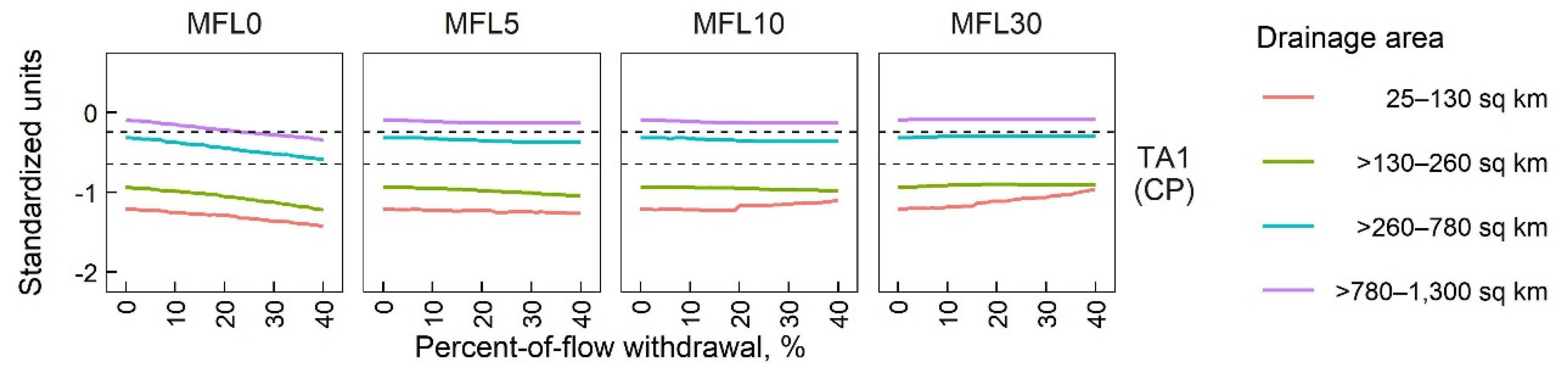
3.1.2. Sensitivity of SFCs to POF Withdrawals

Mean sensitivities of SFC for MFL0 indicated that some SFCs were generally less sensitive to POF withdrawals than CR withdrawals, particularly TL1 (timing), LDH13 and TA1 (flow ratio), LDL6, LDH16 and FL2 (flow variability), FH6 (frequency), and LRA7 (magnitude) (Table 2; Figures S5–S8). In contrast to CR withdrawals, TL1 and LDL6 were not sensitive to POF withdrawals under MFL0 (Table 2). Additionally, underlying patterns of most SFC responses to POF withdrawals were largely monotonic across sites, ecoregions, and MFLs. Responses of streams with relatively small drainage area were also often similar and/or proportional to those with larger drainage area (e.g., TA in Figure 5 and Figures S5–S8).

Decreases in mean sensitivity of TA1, ML20, MA41, LDH13, and LRA7 (Table 2) among MFLs indicate the presence of some damping effects under POF withdrawals, in which TA1 (Figure 5) appeared to have relatively stronger and more consistent damping effects compared to others SFCs across respective ecoregions. However, compared to CR withdrawals, damping effects under POF withdrawals were generally weaker and less consistent among most SFCs. Damping effects appeared to be absent among TL1, LDL6, FH6, LDH16, FL2, and AMH10 (Table 2, Figures S5–S8). Similar to CR withdrawals, some SFCs showed some greater sensitivity at higher MFLs under POF withdrawals, specifically FL2 among RV streams and TL1 among IP streams (Table 2; see example of FL2 in Figure S6 and TL1 in Figure S8).

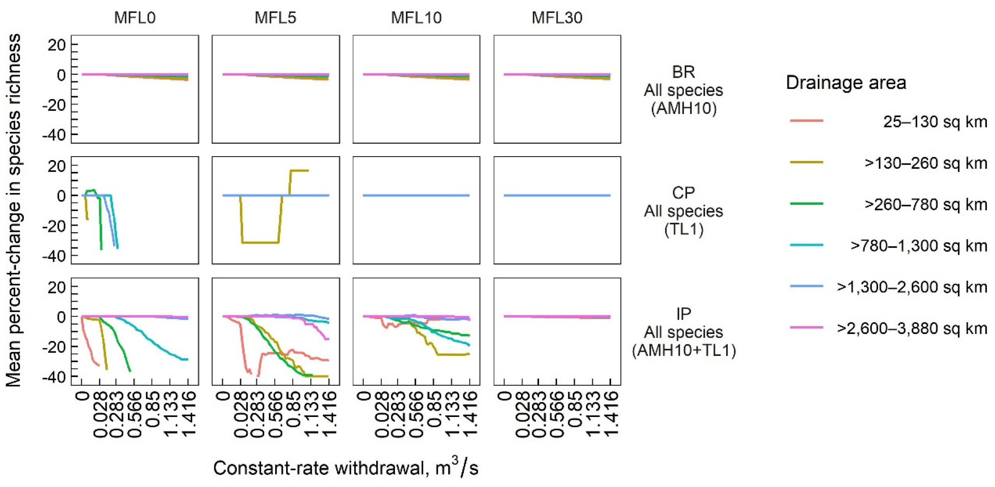
3.2. Species-Richness Responses

Mean changes in richness (averaged among withdrawal scenarios and across stream sites) were negative across most fish groups and MFLs. Compared to CR withdrawals, overall mean loss of richness predicted under POF withdrawals was generally lower across fish groups and ecoregions (

Table 3. Mean change in predicted fish species richness across all stream sites and water-withdrawal scenarios for select fish groups under constant-rate and percent-of-flow withdrawals.

			Constant-Rate Withdrawal Mean Change in Richness				Percent-of-Flow Withdrawal Mean Change in Richness
Eco-Region	Fish Group 1,2,3	Streamflow Characteristic (s)	MFL0	MFL5	MFL10	MFL30	MFL0	MFL5	MFL10	MFL30
BR	All species	AMH10	−0.28	−0.28	−0.28	−0.26	−0.40	−0.40	−0.40	−0.39
RV	All species	FL2	−0.10	−4.89	−5.57	−1.01	0.00	0.00	−0.19	−0.85
	Specialized insectivores	TA1 + LDH16	−0.71	0.94	1.11	0.15	0.51	0.67	0.81	−0.29
CP	All species	TL1	−12.69	−0.02	0.00	0.00	0.00	−0.09	0.00	0.00
	Specialized insectivores	AMH10 + TA1 + TL1	−5.54	0.16	0.01	0.04	−0.25	−0.16	−0.07	0.03
IP	All species	AMH10 + TL1	−21.50	−8.13	−2.97	−0.05	−0.09	−0.52	−0.91	−0.08
	Specialized insectivores	AMH10 + TA1	−0.12	0.53	0.59	0.31	−0.02	0.11	0.21	−0.01

¹ Maximum possible species richness for each fish group is represented by the ‘intercept’ coefficient in Table S1; ² Mean change in richness for all fish groups modelled in this study are presented in Table S2; ³ The identities of fish species within each group were not considered and membership of an individual species to a fish group is not mutually exclusive.

and Table S2).

However, patterns of change in predicted species richness along the withdrawal gradients were highly variable among sites for different fish groups, ecoregions, MFLs, and streams of different drainage-area sizes under both CR (Figures S9–S12) and POF withdrawals (Figures S13–S16), in which richness responses were related to the relative individual sensitivity and cumulative departures from reference conditions of SFC(s) that defined the ELF for each combination of fish group and ecoregion.

Under CR withdrawals, overall mean changes in predicted richness ranged from −21.5 species (loss) to 0.02 species (gain) across fish groups for MFL0 (Table S2). The relative magnitude of richness loss was greatest among fish groups influenced by more sensitive SFCs (Table 3 and Table S2). For example, the strongest patterns of both mean change in richness and damping effects of MFLs among stream sites were associated with fish groups influenced by TL1 for CP (10 of 11 fish groups) and IP (6 of 10 fish groups) (e.g., Table 3; see examples of the ‘All species’ fish groups for CP and IP in Figure 6), in which predicted richness losses were generally greater at MFL0 than MFL5−MFL30. In contrast, fish groups that were predominantly (or solely) influenced by SFC(s) that were only relatively weakly sensitive to CR withdrawals and/or MFLs showed correspondingly weak patterns in richness responses across withdrawal scenarios (e.g., BR sites for the ‘All species’ group in Table 3 and Figure 6).

Under POF withdrawals, overall mean changes in predicted richness (averaged across all withdrawal scenarios for each site) ranged from −0.44 to 0.51 species among fish groups for MFL0 (Table S2). Patterns of richness loss under POF withdrawals were less strongly associated with a single SFC (Table 3 and Table S2), compared to CR. With the exception of relatively small decreases in the mean predicted richness loss among some fish groups influenced by TA1 among CP and IP (e.g., specialized insectivores from CP in Table 3), patterns of change in richness among MFLs were largely inconsistent among fish groups and ecoregions (Table S2, Figures S13–S16). These inconsistencies indicated generally lesser damping effects of MFLs on outcomes of species richness under POF withdrawals.

In relation to 10- and 20-percent presumptive standards [30], mean loss in richness across all stream sites for each fish group and ecoregion for MFL0 ranged from 0.01 to 0.66 species at 10% withdrawals and from 0.02 to 1.34 richness loss at 20% daily water withdrawal. The overall mean predicted richness loss collectively among ecoregions was 0.17 and 0.33 species, respectively (

Table 4. Mean loss and mean percent-loss in predicted fish species across stream sites at 10 and 20% (POF) withdrawal scenarios for MFL0. Means calculated only among streams and fish groups that exhibited declines in richness.

		Mean Loss in Richness (Number of Species)				Mean Percent Loss in Richness (%)
		10% Flow Withdrawal		20% Flow Withdrawal		10% Flow Withdrawal		20% Flow Withdrawal
Eco-Region	Number of Fish Groups1	Range	Mean	Range	Mean	Range	Mean	Range	Mean
BR	3	0.11–0.32	0.19	0.16–0.43	0.27	0.85–0.99	0.93	1.20–1.34	1.29
RV	2	0.34–0.43	0.39	0.61–0.81	0.71	3.86–10.59	7.23	7.31–13.19	10.25
CR	9	0.02–0.31	0.13	0.05–0.61	0.30	0.75–12.95	3.45	1.28–18.89	7.67
IP	10	0.01–0.66	0.15	0.02–1.34	0.29	0.15–7.12	1.34	0.22–13.00	2.57
Overall Mean			0.17		0.33		2.57		4.96

¹ Mean values for each fish group presented in Table S3.

and Table S3). Mean percent loss in species richness among fish groups ranged from 0.15% to 12.95% at 10% withdrawal and from 0.22% to 18.89% at 20% withdrawals, with an overall mean percent richness loss of 2.57% and 4.96%, respectively, across all fish groups and ecoregions (Table 4 and Table S3).

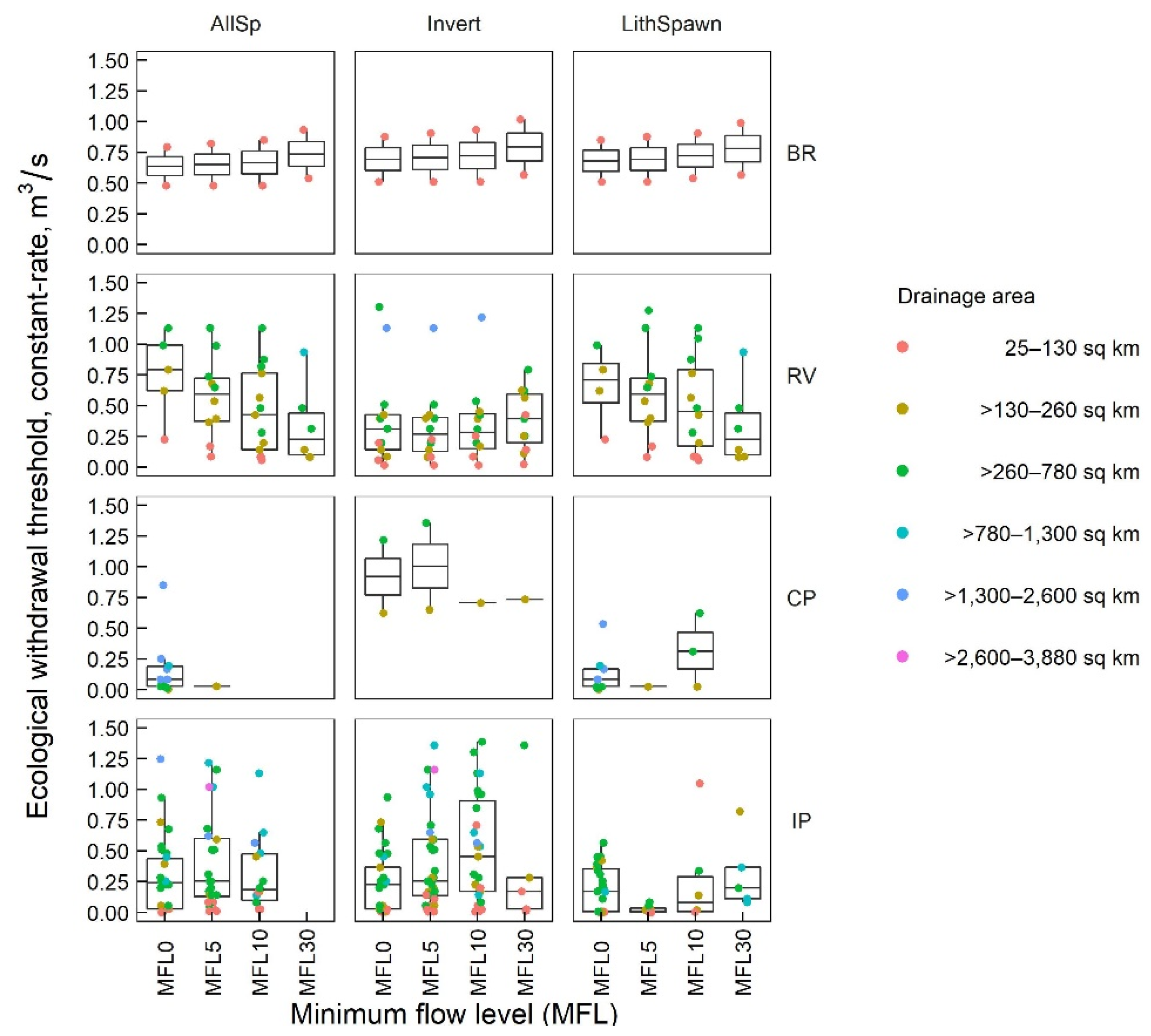
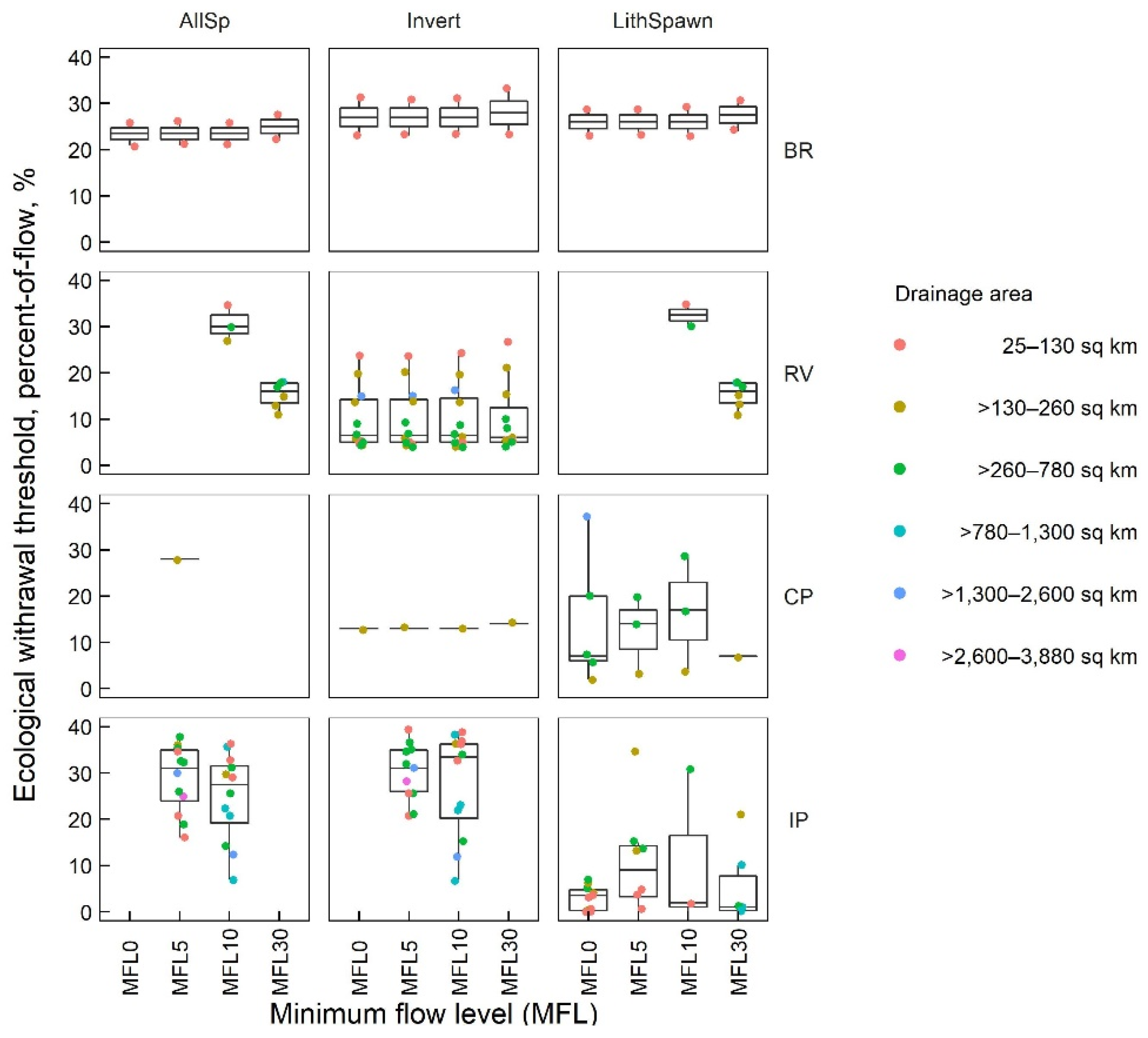
3.3. Ecological Withdrawal Thresholds

3.3.1. CR Withdrawal Scenarios

Box plots of ecological withdrawal thresholds from select fish groups under CR withdrawals show a high degree of variability among stream sites both within and among drainage-area sizes, MFLs, and ecoregions (Figure 7 and Figure S17). Despite considerable variability of thresholds among streams of the same drainage-area size, relatively smaller-size streams often were associated with lower thresholds compared to larger-size streams across fish groups (Figure 7 and Figure S17). For MFL0, median thresholds ranged from 0.01–0.92 m³/s across all fish groups and ecoregions, and median thresholds were often higher among BR and RV fish groups compared to CP and IP (

Table 5. Range and mean of median values (across fish groups) of predicted ecological withdrawal thresholds under constant-rate (m³/s) and percent-of-flow (%) withdrawal scenarios for each ecoregion. “n” = cumulative number (sum) of sites that reached an ecological withdrawal threshold across all fish groups for each ecoregion.

Constant-Rate (CR) Ecological Withdrawal Thresholds (m3/s) 1
	MFL0			MFL5			MFL10			MFL30
Eco-Region	n 2	Range	Mean	n	Range	Mean	n	Range	Mean	n	Range	Mean
BR	6	0.64−0.68	0.67	6	0.64−0.68	0.68	6	0.67−0.72	0.70	6	0.74−0.79	0.77
RV	47	0.20−0.81	0.62	73	0.24−0.68	0.51	80	0.06−0.64	0.39	52	0.23−0.57	0.34
CP	98	0.01−0.92	0.16	25	0.03−1.01	0.23	23	0.01−0.92	0.35	11	0.03−0.85	0.40
IP	267	0.17−0.37	0.23	187	0.10−0.37	0.20	118	0.17−0.37	0.26	33	0.17−1.33	0.67
Percent-of-flow (POF) ecological withdrawal thresholds (%) 1
	MFL0			MFL5			MFL10			MFL30
Eco-region	n 2	Range	Mean	n	Range	Mean	n	Range	Mean	n	Range	Mean
BR	6	23.5−27.0	25.5	6	23.5−27.0	25.5	6	23.5−27.0	25.5	6	25.0−28.0	26.8
RV	17	6.0−6.5	6.3	16	6.5−14.5	10.5	25	1.0−32.5	22.9	49	6.0−16.0	13.0
CP	33	4.0−16.0	9.4	29	4.0−28.0	15.7	22	4.0−29.0	13.7	14	2.0−17.0	7.6
IP	63	3.5−31.0	18.8	102	9.0−31.0	22.6	76	2.0−33.5	18.6	23	1.0−37.0	14.7

¹ Median threshold values and the number of sites (n) for each fish group are presented in Table S4; ² Sites that reached a threshold in multiple fish groups were counted more than once, meaning cumulative “n” can be greater than the number of individual stream sites for each ecoregion.

). For MFL0, the relatively higher number of stream sites that reached an ecological withdrawal threshold and the relatively lower threshold values among CP and IP fish groups (compared to BR and RV) (Table 5) were associated with the prevalence and influence of TL1 among fish groups (Table S4). In partial support of our hypothesis, the reduced number of sites that reached a threshold among MFL5–MFL30 in relation to MFL0 among most fish groups for CP and IP indicated damping effects and suggested that some sites became less sensitive to loss of species richness as MFLs increased under CR withdrawals (Table 5 and Table S4; Figures S11 and S12). For example, the cumulative number of ecological withdrawal thresholds reached among stream sites across fish groups for IP decreased from 267 under MFL0 to 187, 118, and 33 under MFL5, MFL10, MFL30, respectively (Table 5 and Table S4). Counter to predictions, however, the number of thresholds reached among most RV fish groups tended to increase and threshold values tended to decrease with increasingly protective MFLs, related to the influence of FL2 among RV fish groups, in which FL2 showed greater sensitivity to CR withdrawals at higher MFLs (Table 5 and Table S4; Figures S2 and S10).

3.3.2. POF Withdrawal Scenarios

Under POF scenarios, patterns of ecological withdrawal thresholds were also variable among drainage-area sizes, MFLs, and ecoregions and spanned the entire gradient, from 0 to 40% of the mean daily streamflow (Figure 8 and Figure S18). For MFL0, median thresholds ranged from 3.5 to 31% of the daily withdrawal among all fish groups and ecoregions (Table 5), with most fish group median thresholds < 20% daily withdrawal (Table S4). Compared to CR withdrawals, the cumulative number of stream sites that reached an ecological withdrawal threshold under POF withdrawals was consistently lower for MFL0 among fish groups and ecoregions (Table 5), indicating generally reduced sensitivity of stream sites to species richness loss (i.e., 5% biological response limit). Decreases in the number of thresholds reached at MFL5–MFL30 in relation to MFL0 among fish groups influenced predominantly by TA1 among RV, CP, and IP ecoregions indicate some damping effects of MFLs (Table S4).

4. Discussion

Despite some variability among ecoregions, fish groups, and SFCs, our findings generally indicate that POF withdrawals better preserved aspects of the baseline flow regime and had overall less negative impacts on fish species richness compared to CR withdrawals. In general, CR withdrawals resulted in greater sensitivity of SFCs across several ecoregions compared to POF withdrawals, particularly for metrics associated with low streamflows. Similarly, CR withdrawals produced greater sensitivity of SFCs to the protective effects of MFLs. CR withdrawals also resulted in more frequent instances of predicted declines in species richness with greater simulated withdrawals. This included greater overall numbers of sites that reached an ecological withdrawal threshold corresponding to loss of at least 5% species richness at some point along the simulated water-withdrawal gradient. In contrast, POF withdrawals resulted in lower sensitivity, or in some cases, a lack of sensitivity of SFCs related to variability and timing of streamflows, lower sensitivity of SFCs and species richness to MFLs, and relatively fewer ecological withdrawal thresholds reached among streams across fish groups and ecoregions. These findings support the notion that different water-withdrawal strategies can have important hydrologic and ecologic consequences [5,30] and our findings are consistent with other studies demonstrating the potential benefits of POF-type water-management strategies [1,30].

Under both CR and POF withdrawal strategies, the sensitivity of SFCs to withdrawals and the resulting changes in predicted species richness showed apparent relations to drainage area, with smaller streams showing greater sensitivity to water withdrawals than larger streams. Hydrologic and ecologic structuring along stream-size gradients is well documented [54] and classifying streams by size and/or hydrologic regime is often a critical step in developing ecological-flow relationships [22]. A similar study conducted recently among streams in Virginia, suggests that stream size (e.g., drainage area) may be one of the most important factors influencing patterns of change in species richness associated with alteration of streamflows (personal communication, J. Rapp, USGS Virginia/West Virginia Water Science Center, Richmond, VA, USA). Similarly, a study that investigated potential impacts of water withdrawals among streams within the Marcellus Shale region in West Virginia and Pennsylvania, indicates that streams with a drainage area greater than 1000 km² may be less susceptible to changes in hydrologic indices and potential negative ecological responses [52]. The relatively small number of streams sites within each drainage-area size among ecoregions for our study precluded more detailed comparison of patterns among sizes, but general patterns suggest that stream size is an important factor when considering potential withdrawal thresholds at local and regional scales.

Water-withdrawal simulations in this study generally support the idea that MFLs can provide important protection to ecological flow regimes. Specifically, the damping effects of MFLs on the sensitivities of select SFCs and patterns of change in species richness and ecological withdrawal thresholds under both CR and POF water withdrawals imply that MFLs can help protect against richness loss [1,29,30] and, in some circumstances, may allow for greater water withdrawals with relatively lower ecological impacts. Although other SFCs were also sensitive to the damping effects of MFLs, the prevalence of TL1 and TA1 in ELFs among fish groups and ecoregions and the high sensitivity of these SFCs to withdrawals, particularly under CR withdrawals, appear to be the primary drivers of patterns of ecological withdrawal thresholds among many fish groups, MFLs, and ecoregions. Because low flows are particularly vulnerable to water withdrawals [7,52,55], the high sensitivity of TL1 (as well as LDL6) to CR withdrawals for MFL0 and the limited changes in richness loss observed for MFL5–MFL30 are not surprising and highlight the potential influence of even modest MFLs on mitigating fish species richness loss under CR withdrawal scenarios. However, variable (or lack of) sensitivity of some SFCs to MLFs support the notion that minimum flow cutoffs alone may not be sufficient for protecting against richness loss [1,6,30]. Damping effects of MFLs were less prevalent under POF withdrawals, but the general influence of higher MFLs on TA1 and corresponding fish groups across multiple ecoregions further argues in favor of the potential ecological benefits of applying some form of MFL, regardless of whether CR or POF withdrawals are employed.

Our findings show that increasing CR or POF water withdrawals can result in reductions in fish-species richness within some fish groups at some sites. However, the high degree of variability in predicted species richness responses and the range of ecological withdrawal thresholds identified across local (sites specific) and regional (ecoregion) scales suggests that application of these results for management decisions should be implemented with caution. For example, median withdrawal thresholds predicted under CR withdrawals for MFL0 (Table 5 and Table S4) were substantially higher than a large majority of annual mean-monthly withdrawal rates reported for nearly 800 permitted water-withdrawal facilities within the State of Tennessee during 2010 [50], of which the median withdrawal value was approximately 0.013 m³/s. Although the 2010 withdrawal data used by [50] is now somewhat dated, and reported withdrawals may often be less than permitted withdrawals [56], these data suggest that many of the withdrawal thresholds predicted under CR withdrawals in this study would greatly exceed the reported withdrawal rates of many water-use facilities. As a site-specific example, the lowest ecological withdrawal threshold predicted for Yellow Creek at Ellis Mills, TN (ecoregion = Interior Plateau; USGS station number = 03436690; drainage area = 237 km²), was 0.396 m³/s [53], whereas the annual mean monthly withdrawal rate reported by a public supply facility that withdraws surface water from Yellow Creek near the USGS gauge was several orders of magnitude lower: 0.0008 m³/s [50]. Additionally, site-specific ecological withdrawal thresholds were often much greater than 7Q10 flows (annual 7-day minimum flow with a 10-year recurrence interval) [53], a metric commonly used by water-management agencies for assessing water-withdrawal limits. On the one hand, these results could be interpreted as general evidence that some existing withdrawal rates could be increased; however, a more cautious interpretation, and more likely, is that the CR withdrawal model may not fully capture the potential ecological responses to increasing withdrawals among many stream sites, particularly at lower CR withdrawal rates. Overall, the magnitudes of ecological withdrawal thresholds predicted under CR withdrawals for many stream sites and for most fish groups exceeded real-world water-withdrawal rates. This indicates that the applicability of specific CR withdrawal thresholds for management decisions is limited and should be interpreted with caution.

Regarding POF withdrawal scenarios, the range of median thresholds summarized among fish groups and ecoregions is largely consistent with the range of recommended limits to daily POF streamflow reductions (approximate 6–35%) reported among several empirical case studies (e.g., [57,58,59], and summarized in [30]. The mean percent loss in species richness among fish groups for across ecoregions at 10 and 20 POF withdrawal scenarios (Table 4 and Table S3) are generally supportive of Richter’s [30] presumptive flow standards, and are also in agreement with the use of 5% loss in richness as a conservative biological response limit. However, richness losses greater than 5% among some fish groups indicate that POF withdrawal rates less than 10 or 20% of daily streamflow may be necessary to protect particularly sensitive fish groups or species (e.g., specialized insectivores (RV, CP), intolerant species (CP), and lithophilic spawners (IP) in Table S3). Further, overall averages of mean percent loss and mean absolute loss in species richness for 10 and 20 POF withdrawal scenarios were similar to or lower than those predicted for streams throughout North Carolina [36] and are in agreement with findings for streams in Virginia (personal communication, J. Rapp, USGS Virginia/West Virginia Water Science Center, Richmond, VA, USA). Specifically, [36] predicted a loss of 0.49 and 1.0 fish species for flow reduction scenarios of 15% and 25% among streams in North Carolina, whereas the predicted loss of richness at 20% withdrawals among fish groups and ecoregions in our study was often much less than 0.5 species and averaged only 0.33 species across groups (Table 4). Although the methods and criteria for developing flow-ecology relationships differed between our study and others [36], similarities in predicted ecological outcomes at 10 and 20% flow reductions suggest that these POF withdrawal rates may be generally applicable among basins and ecoregions of the southeastern U.S.

Our data indicated that protection of low stream flows, specifically timing of low flows, was particularly important for steams and fish groups within CP and IP ecoregions. Others have shown that low-flow metrics may be particularly sensitive to water withdrawals [52]. Water withdrawals can exacerbate low-flow conditions and alteration of the timing, magnitude, duration, and frequency of low flows are known to have negative impacts on aquatic biota, stream habitat, and water quality [2,5,7,55]. Intensification of low-flow conditions can impact fish species and communities at local and regional scales through increased mortality and disruption of reproduction, recruitment, and dispersal [2,7,60]. Nuisance and/or harmful algal blooms (HABs) and associated decreases in dissolved oxygen often occur during low flows, and cyanobacteria HABs and toxicity in lotic ecosystems are an increasing management concern in some regions [61,62]. Use of percentage-of-flow and presumptive standards are increasingly popular among water-management agencies within the US and elsewhere [30,57,63,64]. Despite high variability in the ecological withdrawal thresholds among stream sites and variability in responses among fish groups, our data provide support for water-management strategies using POF withdrawals and the implementation of MFLs to help mitigate hydrologic alteration and negative impacts on fish species richness.

Considerations and Caveats of Water-Withdrawal Models

The importance of SFC selection when characterizing ecologically relevant aspects of the flow regime is well recognized [1,65], as is the potential variability in sensitivities of SFCs to hydrologic alteration [46,52]. Although the ecological and statistical relevance of specific SFCs used in this study have been previously described for streams within the Cumberland and Tennessee River basins [37,38,39,41], the potential sensitivities of these SFCs to CR and POF water withdrawals and MFL scenarios were not specifically considered in previous works. SFCs that had greater individual sensitivity to withdrawals and are of demonstrated importance to fish communities may be particularly important targets for water-management decisions. On the other hand, SFCs with limited sensitivity to CR or POF withdrawals in this study may still be important and warrant attention from resource managers under different flow alteration conditions than considered in this study. In the Tennessee and Cumberland River basins, TL1 and TA1 were of particular ecological importance, but other SFCs may be more important in other regions or other climate contexts [8].

Ecological withdrawal thresholds summarized across sites according to drainage area, fish groups, or cumulatively for each ecoregion using central tendencies (e.g., median or means), may be as or more valuable than site-specific thresholds for use in decision making at local and regional scales. Specifically, summarized thresholds may inform decisions regarding water withdrawals among streams. Although site-specific withdrawal thresholds [53] may be useful for specific stream systems, in which species richness responses and thresholds modeled independently for each fish group and MFL represent multiple lines of evidence to guide management decisions, high variability at the individual site level may confound decision making.

Modelled hydrologic and ecological responses to increasing CR and POF water-withdrawal scenarios were based on underlying flow-ecology relationships that assume that patterns of fish species richness are determined solely by streamflow and that responses would be generally linear. However, non-linear responses are common in natural systems [64], and although [39] found some evidence of internal structuring of species-richness responses presumed to be associated with factors other than streamflow (e.g., water quality, physical habitat), the influence of additional environmental factors in determining fish species richness were not considered in this study.

Daily streamflow data used to calculate water-withdrawal scenarios from USGS streamgauge sites were assumed to represent the baseline (i.e., unaltered) flow regime for each site, and the simulated water withdrawals modelled in this study were assumed to be the only source of streamflow alteration during the period of record for each site. However, we acknowledge that this assumption ignores additional real-world sources of streamflow alteration, including effects of previous or existing flow alterations and cumulative effects of upstream withdrawals or effluent discharges on downstream sites.

Quantile regression results used in prior studies to develop the ELFs used in this study provide regional expected upper-bound predictions of fish species richness in relation to the departure of SFCs from defined hydrologic reference conditions. Some stream sites may fit regional ELF equations better than others, depending on the relative position of specific SFCs under the initial baseline flow regime to that of the defined reference condition. For example, when subjected to water withdrawals, a calculated baseline SFC value that was initially greater than the so-called reference condition may move closer to the reference condition (i.e., decreased departure), and can result, mathematically, in an increase in predicted species richness. While it is ecologically plausible that some species may benefit from reductions in streamflow under certain conditions, large increases in predicted fish species richness with increasing water withdrawals were not considered realistic outcomes and thus were largely ignored in this study. Actual gains in species richness would likely be limited to a modest number of potential colonists by natural abiotic (i.e., physical and chemical habitat limitations), biotic (e.g., competition), and spatial mechanisms (e.g., distance or dispersal barriers) [66]. A review among 165 empirical studies by [5] found that only 13% of the studies reported some positive association between ecological metrics and flow alteration. In this study, some sites exhibited no change in predicted richness under any simulated water-withdrawal scenario. These results should also be interpreted with caution because it is unrealistic to assume that fish species richness would be categorically unaffected by increasingly large withdrawals.

Predicted loss (or gain) of fish species at any given stream site was relative to the predicted richness under baseline streamflow (i.e., simulated withdrawal = 0 m³/s) which was produced by a regionalized quantile regression curve, assuming >85% probably of species richness at ‘optimal’ or reference conditions [39]. If the initial baseline flow conditions are far from reference conditions, the actual fish species richness that exists at any given stream may be different than what is predicted using the given ELF equations. Additionally, stream size was not considered during the initial development of ELFs, which means that the same ELF equation is used to predict richness among streams regardless of stream size. For example, a stream with a drainage area size of 10 km² could be predicted to have the same or even greater richness than a stream with a drainage area of 1,000 km² in the same ecoregion, depending on the hydrologic departure from reference of the subset of SFCs that define each ELF.

5. Conclusions

Results of this study indicate that increasing water-withdrawal rates, regardless of the withdrawal strategy, will likely result in increased loss of fish species richness across a variety of streams and ecoregions. However, the alteration of hydrologic regimes and the resulting predicted richness losses were generally less severe under the POF water withdrawals compared to CR withdrawals, suggesting potential benefits of POF withdrawal scenarios in maintaining aquatic biodiversity. Richness losses and patterns among ecological withdrawal thresholds under POF withdrawals showed general concurrence with Richter’s [30] presumptive standards and suggest that limiting water withdrawals to 10–20% of daily streamflow may indeed be generally protective of species richness among most stream drainage area sizes and ecoregions. The sensitivity of low-flow SFCs to CR withdrawals and the prevalence of the low-flow metrics among ELFs across ecoregions suggests that protocols for protection of low flows, such as MFL cutoffs, are likely critical when CR water-withdrawal strategies are employed. Our findings also showed that application of MFL cutoffs, regardless of the withdrawal strategy, were generally effective at damping hydrologic alteration and species richness responses to both withdrawal strategies and indicate that employing MFLs may allow for larger permitted water withdrawals under some circumstances. Development of specific and practical guidelines that limit water withdrawals within ecological response boundaries have been difficult to achieve. This study provides a general framework of comparative and alternative potential outcomes under plausible water-withdrawal strategies. Localized and regionalized estimates of predicted hydrologic and ecologic responses generated in this study could be useful for informing resource management and policy decisions. Lastly, more detailed prioritization of sensitive ecoregions, geographical areas, sub-watersheds, and streams of a certain size or drainage area is an important next step in guiding more targeted management and conservation strategies and actions.

References

1. Poff, N.L.; Allan, J.D.; Bain, M.B.; Karr, J.R.; Prestegaard, K.L.; Richter, B.D.; Sparks, R.E.; Stromberg, J.C. The natural flow regime. BioScience 1997, 47, 769–784. [Google Scholar] [CrossRef]
2. Bunn, S.E.; Arthington, A.H. Basic principles and ecological consequences of altered flow regimes for aquatic biodiversity. Environ. Manag. 2002, 30, 492–507. [Google Scholar] [CrossRef] [PubMed] [Green Version]
3. Tharme, R.E. A global perspective on environmental flow assessment: Emerging trends in the development and application of environmental flow methodologies for rivers. River Res. Appl. 2003, 19, 397–441. [Google Scholar] [CrossRef]
4. Dudgeon, D.; Arthington, A.H.; Gessner, M.O.; Kawabata, Z.-I.; Knowler, D.J.; Lévêque, C.; Naiman, R.J.; Prieur-Richard, A.-H.; Soto, D.; Stiassny, M.L.J.; et al. Freshwater biodiversity: Importance, threats, status and conservation challenges. Biol. Rev. 2006, 81, 163–182. [Google Scholar] [CrossRef]
5. Poff, N.L.; Zimmerman, J.K.H. Ecological responses to altered flow regimes: A literature review to inform the science and management of environmental flows. Freshw. Biol. 2010, 55, 194–205. [Google Scholar] [CrossRef]
6. Annear, T.; Chisholm, I.; Beecher, H.; Locke, A.; Aarrestad, P.; Coomer, C.; Estes, C.; Hunt, J.; Jacobson, R.; Jobsis, G.; et al. Instream Flows for Riverine Resource Stewardship, Revised ed.; Instream Flow Council: Cheyenne, WY, USA, 2004. [Google Scholar]
7. Rolls, R.J.; Leigh, C.; Sheldon, F. Mechanistic effects of low-flow hydrology on riverine ecosystems: Ecological principles and consequences of alteration. Freshw. Sci. 2012, 31, 1163–1186. [Google Scholar] [CrossRef] [Green Version]
8. Walters, A.W. The importance of context dependence for understanding the effects of low-flow events on fish. Freshw. Sci. 2016, 35, 216–228. [Google Scholar] [CrossRef] [Green Version]
9. Doll, P.; Fiedler, K.; Zhang, J. Global-scale analysis of river flow alterations due to water withdrawals and reservoirs. Hydrol. Earth Syst. Sci. 2009, 12, 2413–2432. [Google Scholar] [CrossRef] [Green Version]
10. Robinson, J. Public-Supply Water Use and Self-Supplied Industrial Water Use in Tennessee, 2010; U.S. Geological Survey Scientific Investigation Report 2018–5009; U.S. Geological Survey: Reston, VA, USA, 2018; p. 30.
11. Shen, Y.; Oki, T.; Utsumi, N.; Kanae, S.; Hanasaki, N. Projection of future world water resources under SRES scenarios: Water withdrawal. Hydrolog. Sci. J. 2008, 53, 11–33. [Google Scholar] [CrossRef] [Green Version]
12. Meador, M.R.; Carlisle, D.M. Relations between altered streamflow variability and fish assemblages in eastern USA streams. River Res. Appl. 2012, 28, 1359–1368. [Google Scholar] [CrossRef]
13. Phelan, J.; Cuffney, T.; Patterson, L.; Eddy, M.; Dykes, R.; Pearsall, S.; Goudreau, C.; Mead, J.; Tarver, F. Fish and invertebrate flow-biology relationships to support the determination of ecological flows for North Carolina. J. Am. Water Resour. As. 2017, 53, 42–55. [Google Scholar] [CrossRef]
14. Freeman, M.C.; Marcinek, P.A. Fish assemblage responses to water withdrawals and water supply reservoirs in Piedmont streams. Environ. Manag. 2006, 38, 435–450. [Google Scholar] [CrossRef] [PubMed]
15. Kanno, Y.; Vokoun, J.C. Evaluating effects of water withdrawals and impoundments on fish assemblages in southern New England streams, USA. Fish. Manag. Ecol. 2010, 17, 272–283. [Google Scholar] [CrossRef]
16. Baron, J.S.; Poff, N.L.; Angermeier, P.L.; Dahm, C.N.; Gleick, P.H.; Hairston, N.G.; Jackson, R.B.; Johnston, C.A.; Richter, B.D.; Steinman, A.D. Meeting ecological and societal needs for freshwater. Ecol. Appl. 2002, 12, 1247–1260. [Google Scholar] [CrossRef]
17. Arthington, A.; James, C.; Mackay, S.; Rolls, R.; Sternberg, D.; Barnes, A. Hydro-Ecological Relationships and Thresholds to Inform Environmental Flow Management; Science Report; International WaterCentre: Brisbane, Australia, 2012; p. 224. [Google Scholar]
18. Arthington, A.H.; Bunn, S.E.; Poff, N.L.; Naiman, R.J. The challenge of providing environmental flow rules to sustain river ecosystems. Ecol. Appl. 2006, 16, 1311–1318. [Google Scholar] [CrossRef]
19. Arthington, A.H.; Brizga, S.; Kennard, M. Comparative Evaluation of Environmental Flow Assessment Techniques: Best Practice Framework; LWRRDC Occasional Paper 25/98; Land and Water Resources Research and Development Corporation: Canberra, Australia, 1998; p. 26.
20. Wheeler, K.; Wenger, S.J.; Freeman, M.C. States and rates: Complementary approaches to developing flow-ecology relationships. Freshw. Biol. 2018, 63, 906–916. [Google Scholar] [CrossRef]
21. Acreman, M.C.; Overton, I.C.; King, J.; Wood, P.J.; Cowx, I.G.; Dunbar, M.J.; Kendy, E.; Young, W.J. The changing role of ecohydrological science in guiding environmental flows. Hydrol. Sci. J. 2014, 59, 433–450. [Google Scholar] [CrossRef]
22. Poff, N.L.; Richter, B.D.; Arthington, A.H.; Bunn, S.E.; Naiman, R.J.; Kendy, E.; Acreman, M.; Apse, C.; Bledsoe, B.P.; Freeman, M.C.; et al. The ecological limits of hydrologic alteration (ELOHA): A new framework for developing regional environmental flow standards: Ecological limits of hydrologic alteration. Freshw. Biol. 2010, 55, 147–170. [Google Scholar] [CrossRef] [Green Version]
23. Pastor, A.V.; Ludwig, F.; Biemans, H.; Hoff, H.; Kabat, P. Accounting for environmental flow requirements in global water assessments. Hydrol. Earth Syst. Sci. 2014, 18, 5041–5059. [Google Scholar] [CrossRef] [Green Version]
24. Naiman, R.J.; Bunn, S.E.; Nilsson, C.; Petts, G.E.; Pinay, G.; Thompson, L.C. Legitimizing fluvial ecosystems as users of water: An overview. Environ. Manag. 2002, 30, 455–467. [Google Scholar] [CrossRef]
25. Poff, N.L.; Allan, J.D.; Palmer, M.A.; Hart, D.D.; Richter, B.D.; Arthington, A.H.; Rogers, K.H.; Meyer, J.L.; Stanford, J.A. River flows and water wars: Emerging science for environmental decision making. Front. Ecol. Environ. 2003, 1, 298–306. [Google Scholar] [CrossRef]
26. Davies, P.M.; Naiman, R.J.; Warfe, D.M.; Pettit, N.E.; Arthington, A.H.; Bunn, S.E. Flow–ecology relationships: Closing the loop on effective environmental flows. Mar. Freshw. Res. 2014, 65, 133–141. [Google Scholar] [CrossRef]
27. Cartwright, J.; Caldwell, C.; Nebiker, S.; Knight, R. Putting flow–ecology relationships into practice: A decision-support system to assess fish community response to water-management scenarios. Water 2017, 9, 196. [Google Scholar] [CrossRef]
28. Tennant, D.L. Instream Flow Regimens for Fish, Wildlife, Recreation and Related Environmental Resources. Fisheries 1976, 1, 6–10. [Google Scholar] [CrossRef]
29. Richter, B.; Baumgartner, J.; Wigington, R.; Braun, D. How much water does a river need? Freshw. Biol. 1997, 37, 231–249. [Google Scholar] [CrossRef] [Green Version]
30. Richter, B.D.; Davis, M.M.; Apse, C.; Konrad, C. A presumptive standard for environmental flow protection. River Res. Appl. 2012, 28, 1312–1321. [Google Scholar] [CrossRef]
31. U.S. Environmental Protection Agency Water: Monitoring and Assessment, Section 5.1 Stream Flow. Available online: https://archive.epa.gov/water/archive/web/html/vms51.html (accessed on 2 January 2020).
32. Farmer, W.H.; Over, T.M.; Kiang, J.E. Bias correction of simulated historical daily streamflow at ungauged locations by using independently estimated flow duration curves. Hydrol. Earth Syst. Sci. 2018, 22, 5741–5758. [Google Scholar] [CrossRef] [Green Version]
33. Cook, C.N.; Hockings, M.; Carter, R. (Bill) Conservation in the dark? The information used to support management decisions. Front. Ecol. Environ. 2010, 8, 181–186. [Google Scholar] [CrossRef]
34. Kendy, E.; Apse, C.; Blann, K. A Practical Guide to Environmental Flows for Policy and Planning, with Nine Case Studies in the United States; The Nature Conservancy: Arlington, VA, USA, 2012. [Google Scholar]
35. Davies, S.P.; Jackson, S.K. The biological condition gradient: A descriptive model for interpreting change in aquatic ecosystems. Ecol. Appl. 2006, 16, 1251–1266. [Google Scholar] [CrossRef]
36. Hain, E.F.; Kennen, J.G.; Caldwell, P.V.; Nelson, S.A.C.; Sun, G.; McNulty, S.G. Using regional scale flow-ecology modeling to identify catchments where fish assemblages are most vulnerable to changes in water availability. Freshw. Biol. 2018, 63, 928–945. [Google Scholar] [CrossRef]
37. Knight, R.R.; Brian Gregory, M.; Wales, A.K. Relating streamflow characteristics to specialized insectivores in the Tennessee River Valley: A regional approach. Ecohydrology 2008, 1, 394–407. [Google Scholar] [CrossRef]
38. Knight, R.R.; Gain, W.S.; Wolfe, W.J. Modelling ecological flow regime: An example from the Tennessee and Cumberland River basins. Ecohydrology 2012, 5, 613–627. [Google Scholar] [CrossRef]
39. Knight, R.R.; Murphy, J.C.; Wolfe, W.J.; Saylor, C.F.; Wales, A.K. Ecological limit functions relating fish community response to hydrologic departures of the ecological flow regime in the Tennessee River basin, United States. Ecohydrology 2014, 1262–1280. [Google Scholar] [CrossRef]
40. Murphy, J.C.; Knight, R.R.; Wolfe, W.J.; S. Gain, W. Predicting ecological flow regime at ungaged sites: A comparison of methods. River Res. Appl. 2012, 29, 660–669. [Google Scholar] [CrossRef]
41. Knight, R.R.; Cartwright, J.M.; Ladd, D.E. Streamflow and Fish Community Diversity Data for Use in Developing Ecological Limit Functions for the Cumberland Plateau, Northeastern Middle Tennessee and Southwestern Kentucky, 2016; U.S. Geological Survey data release; U.S. Geological Survey: Reston, VA, USA, 2016. Available online: http://dx.doi.org/10.5066/F7JH3J83 (accessed on 1 September 2018).
42. Omernik, J.M. Map Supplement: Ecoregions of the Conterminous United States. Ann. Assoc. Am. Geogr. 1987, 77, 118–125. [Google Scholar] [CrossRef]
43. Abell, R.; Olson, D.; Dinerstein, E.; Hurley, P.; Diggs, J.; Eichbaum, W.; Walters, S.; Wettengel, W.; Allnutt, T.; Loucks, C.; et al. Freshwater Ecoregions of North America: A Conservation Assessment; Island Press: Washington, DC, USA, 2000. [Google Scholar]
44. Elkins, D.C.; Sweat, S.C.; Hill, K.S.; Kuhajda, B.R.; George, A.L.; Wenger, S.J. The Southeastern Aquatic Biodiversity Conservation Strategy. Final Report; University of Georgia River Basin Center: Athens, Greece, 2016; p. 237. [Google Scholar]
45. Fenneman, N.M. Physiographic Divisions of the United States. Ann. Assoc. Am. Geogr. 1928, 18, 261. [Google Scholar] [CrossRef]
46. Kennard, M.J.; Mackay, S.J.; Pusey, B.J.; Olden, J.D.; Marsh, N. Quantifying uncertainty in estimation of hydrologic metrics for ecohydrological studies. River Res. Appl. 2010, 137–156. [Google Scholar] [CrossRef]
47. U.S. Geological Survey (USGS) USGS Water Data for the Nation: U.S. Geological Survey National Water Information System Database. Available online: http://dx.doi.org/10.5066/F7P55KJN (accessed on 1 September 2018).
48. Hirsch, R.; De Cicco, L. User Guide to Exploration and Graphics for RivEr Trends (EGRET) and dataRetrieval: R Packages for Hydrologic Data; U.S. Geological Survey Techniques and Methods book 4, chap. A10; U.S. Geological Survey: Reston, VA, USA, 2015; p. 93.
49. R Core Team R: A Language and Environment for Statistical Computing; R Foundation for Statistical Computing: Vienna, Austria, 2019.
50. Robinson, J.A. Water Use in Tennessee, 2010; U.S. Geological Survey data release; U.S. Geological Survey: Reston, VA, USA, 2017. Available online: https://doi.org/10.5066/F7V9868K (accessed on 1 September 2018).
51. Mills, J.; Blodgett, D. EflowStats: Hydrologic Indicator and Alteration Stats. R Package Version 5.0.0; 2017; Available online: https://github.com/USGS-R/EflowStats (accessed on 1 September 2017).
52. Buchanan, B.; McManamay, R.A.; Auerbach, D.; Fuka, D.; Walter, M. Environmental Flow Analysis for the Marcellus Shale Region; Appalachian Landscape Conservation Cooperative: Shepherdstown, WV, USA, 2015; p. 170. [Google Scholar]
53. Driver, L.J. Ecological Flow Analyses Results: Streamflow Characteristics, Predicted Fish Responses, and Ecological Withdrawal Thresholds for Select Stream Sites within the Cumberland and Tennessee River Basins; U.S. Geological Survey data release; U.S. Geological Survey: Reston, VA, USA, 2019. Available online: https://doi.org/10.5066/F7Q23Z4B (accessed on 1 September 2019).
54. Vannote, R.L.; Minshall, G.W.; Cummins, K.W.; Sedell, J.R.; Cushing, C.E. The River Continuum Concept. Can. J. Fish. Aquat. Sci. 1980, 37, 130–137. [Google Scholar] [CrossRef]
55. Poff, N.L.; Ward, J.V. Implications of Streamflow Variability and Predictability for Lotic Community Structure: A Regional Analysis of Streamflow Patterns. Can. J. Fish. Aquat. Sci. 1989, 46, 1805–1818. [Google Scholar] [CrossRef]
56. Shank, M.K.; Stauffer, J.R. Land use and surface water withdrawal effects on fish and macroinvertebrate assemblages in the Susquehanna River basin, USA. J. Freshw. Ecol. 2015, 30, 229–248. [Google Scholar] [CrossRef] [Green Version]
57. Flannery, M.S.; Peebles, E.B.; Montgomery, R.T. A percent-of-flow approach for managing reductions of freshwater inflows from unimpounded rivers to Southwest Florida estuaries. Estuaries 2002, 25, 1318–1332. [Google Scholar] [CrossRef]
58. Acreman, M.C.; Ferguson, A.J.D. Environmental flows and the European Water Framework Directive: Environmental flows and WFD. Freshw. Biol. 2010, 55, 32–48. [Google Scholar] [CrossRef]
59. Zorn, T.G.; Seelbach, P.W.; Rutherford, E.S.; Wills, T.; Cheng, S.; Wiley, M. A Regional-Scale Habitat Suitability Model to Assess the Effects of Flow Reduction on Fish Assemblages in Michigan Streams; Michigan Department of Natural Resources: Ann Arbor, MI, USA, 2008; pp. 871–895.
60. Driver, L.J.; Hoeinghaus, D.J. Spatiotemporal dynamics of intermittent stream fish metacommunities in response to prolonged drought and reconnectivity. Mar. Freshw. Res. 2016, 67, 1667–1679. [Google Scholar] [CrossRef]
61. Loftin, K.A.; Clark, J.M.; Journey, C.A.; Kolpin, D.W.; Van Metre, P.C.; Carlisle, D.; Bradley, P.M. Spatial and temporal variation in microcystin occurrence in wadeable streams in the southeastern United States: Microcystins in southeastern US streams. Environ. Toxicol. Chem. 2016, 35, 2281–2287. [Google Scholar] [CrossRef] [PubMed]
62. Graham, J.L.; Dubrovsky, N.M.; Foster, G.M.; King, L.R.; Loftin, K.A.; Rosen, B.H.; Stelzer, E.A. Cyanotoxin occurrence in large rivers of the United States. Inland Waters 2020, 10, 109–117. [Google Scholar] [CrossRef]
63. North Carolina Ecological Flows Science Advisory Board. Recommendations for Estimating Flows to Maintain Ecological Integrity in Streams and Rivers in North Carolina; North Carolina Department of Environmental Quality: Raleigh, NC, USA, 2013. Available online: https://files.nc.gov/ncdeq/Water%20Resources/files/eflows/sab/EFSAB_Final_Report_to_NCDENR.pdf (accessed on 4 January 2019).
64. Rosenfeld, J.S. Developing flow-ecology relationships: Implications of nonlinear biological responses for water management. Freshw. Biol. 2017, 62, 1305–1324. [Google Scholar] [CrossRef] [Green Version]
65. Olden, J.D.; Poff, N.L. Redundancy and the choice of hydrologic indices for characterizing streamflow regimes. River Res. Appl. 2003, 19, 101–121. [Google Scholar] [CrossRef]
66. Jackson, D.A.; Peres-Neto, P.R.; Olden, J.D. What controls who is where in freshwater fish communities–the roles of biotic, abiotic, and spatial factors. Can. J. Fish. Aquat. Sci. 2001, 58, 157–170. [Google Scholar] [CrossRef]
Figure 1. Distribution of selected stream sites within Level III ecoregions of the Tennessee and Cumberland River basins.
Water 12 01334 g001
Figure 2. Example daily hydrographs of (a) constant-rate and (b) percent-of-flow water-withdrawal scenarios and minimum flow levels (MFLs). MFL0 hydrographs represent the absence of any MFL protection; MFL5 represents a MFL set at 5% of the mean annual flow. Daily streamflow values extending below y-axis represent flows at or near 0 m3/s on log10 scale.
Water 12 01334 g002
Figure 3. Hypothetical responses of (a) SFC values and (b) percent-changes in species richness plotted for a single stream site across increasing water-withdrawal scenarios and for different minimum flow levels (solid lines). (a) Dashed horizontal lines represent the pre-defined interquartile range of SFC responses among reference sites. (b) Dashed horizontal line represents an arbitrary biological response limit; Dashed red vertical lines represent intersection points at which an ecological withdrawal threshold occurs, i.e., at which a 5% loss of species richness occurs.
Water 12 01334 g003
Figure 4. Mean responses of select streamflow characteristics (SFCs) to incremental constant-rate withdrawal scenarios and minimum flow levels (MFL) within the Cumberland Plateau (CP). Solid lines represent the mean SFC response across sites for each drainage-area size; horizontal dashed lines are the interquartile range (IQR) of SFCs from reference sites within each ecoregion [38,39,41].
Water 12 01334 g004
Figure 5. Mean responses of select streamflow characteristics to incremental percent-of-flow withdrawal scenarios and minimum flow levels (MFL) within the Cumberland Plateau (CP). Solid lines represent mean values across sites for each drainage-area size; horizontal dashed lines are the interquartile range (IQR) of SFCs from reference sites within the ecoregion [38,39,41].
Water 12 01334 g005
Figure 6. Patterns of mean percent change in fish species richness in response to incremental constant-rate withdrawal scenarios and minimum flow levels (MFL) for the “All Species” fish group for Blue Ridge (BR), Cumberland Plateau (CP), and Interior Plateau (IP) ecoregions. Solid lines represent individual stream sites. SFC(s) associated with the ecological limit function for each fish group and ecoregion are in parentheses.
Water 12 01334 g006
Figure 7. Boxplots of predicted ecological withdrawal thresholds under constant-rate withdrawal scenarios among select fish groups and minimum flow levels (MFLs) for Blue Ridge (BR), Ridge and Valley (RV), Cumberland Plateau (CP), and Interior Plateau (IP) ecoregions. Boxes represent the 25th and 75th quantile; center line represents the median (50th percentile). Points are threshold values for individual stream sites and are color coded by drainage-area size. Results for all fish groups are illustrated in Figure S17.
Water 12 01334 g007
Figure 8. Boxplots of predicted ecological withdrawal threshold under percent-of-flow (POF) withdrawal scenarios among select fish groups and minimum flow levels (MFLs) for Blue Ridge (BR), Ridge and Valley (RV), Cumberland Plateau (CP), and Interior Plateau (IP) ecoregions. Boxes represent the 25th and 75th quantile; center line represents the median (50th percentile). Points are threshold values for individual stream sites and are color coded by drainage-area size. Results for all fish groups are illustrated in Figure S18.
Water 12 01334 g008