Article

Land Cover and Water Quality Patterns in an Urban River: A Case Study of River Medlock, Greater Manchester, UK

1
Department of Earth & Environmental Sciences, University of Manchester, Manchester M13 9PL, UK
2
School of Environmental Sciences, University of East Anglia, Norwich NR4 7UA, UK
*
Author to whom correspondence should be addressed.
Water 2020, 12(3), 848; https://doi.org/10.3390/w12030848
Submission received: 31 January 2020 / Revised: 11 March 2020 / Accepted: 13 March 2020 / Published: 17 March 2020
(This article belongs to the Special Issue Monitoring, Modelling and Management of Water Quality)

Abstract

:
Urban river catchments face multiple water quality challenges that threaten the biodiversity of riverine habitats and the flow of ecosystem services. We examined two water quality challenges, runoff from increasingly impervious land covers and effluent from combined sewer overflows within a temperate zone river catchment in Greater Manchester, North-West UK. Sub-catchment areas of the River Medlock were delineated from digital elevation models using a Geographical Information System. By combining flow accumulation and high-resolution land cover data within each sub-catchment and water quality measurements at five sampling points along the river, we identified which land cover(s) are key drivers of water quality. Impervious land covers increased downstream and were associated with higher runoff and poorer water quality. Of the impervious covers, transportation networks have the highest runoff ratios and therefore the greatest potential to convey contaminants to the river. We suggest more integrated management of imperviousness to address water quality, flood risk and, urban wellbeing could be achieved with greater catchment partnership working.

1. Introduction

Urban land covers such as infrastructure, urban greenspace and woodland, residential, and industry and commercial covers can modify water quality either by enhancing or reducing runoff [1] and in turn contaminant levels entering freshwaters from surrounding terrestrial ecosystems [2,3]. Changes in land cover from human activities or natural drivers, can both affect the quality of the river catchment and thereby compromise the ecosystem services they provide [2,3]. With increased pressures from population growth and urban sprawl, the challenges to water quality are imminent [4,5]. Contemporary, management strategies include restoring ecohydrological processes [6] to renaturate, remediate, and revitalize urban rivers.
Urbanized areas are often characterized by rapid development, modified or canalized rivers, and a high proportion of impervious land [4,7,8,9,10,11,12]. Urban land cover, particularly, impervious surface covers which prevent infiltration of water to the soil, include transport systems (roads, parking lots), roof tops and residential development are a key indicator of the environmental impacts of urbanisation [3]. Point source pollution collected from impervious urban areas contributes to river flows, changes river hydrology, alters physicochemical processes [13] and degrades assemblages of benthic macroinvertebrates [4,12]. During high flows, combined sewer overflows (CSOs) which collect runoff from impervious land covers are designed to overflow and discharge directly, without treatment, into the receiving water body. CSO discharges can degrade water quality including physicochemical and microbial indicators [14,15,16,17].
In the UK, CSOs have long been recognized as one of the major causes of urban river pollution [18,19,20]. They are also a major contributor to coastal pollution and the UK’s Environment Agency (EA) estimates that 30% of coastal pollution in the North West of England can be attributed to CSOs through a combination of breaches and cumulative impact (see, https://www.unitedutilities.com/services/wastewater-services/bathing-waters/what-are-combined-sewer-overflows/). It is therefore critical to understand the risks associated with CSOs particularly with changing climate and greater future flood risk [21,22,23] and there are challenges in retrofitting CSOs to increase their capacity [23]. Other point source pollution includes industrial effluent, effluent from wastewater treatment works (WwTW), and drainage from agricultural activities.
The application of a Geographic Information System (GIS) to environmental data analyses in river sub-catchments has been explored by researchers [9,10,24,25,26,27]. Studies show that information on land cover patterns can improve our understanding of water quality within catchments [28] and the management of pollution sources [27]. Through ArcGIS tools, topographical characteristics, e.g., slope, flow length, drainage area or catchment area [29,30] that drive surface water flow, can be analyzed through the digital elevation model (DEM) data [31]. DEM data is also used for modelling the urban environment [32] and to delineate catchments for spatial analysis [33,34,35]. Such information is critical for urban river quality management. Additionally, partnership working can be decisive in urban settings, where partnership groups can coordinate across: Threats, policy domains, e.g., land and water management, urban re/development including integration with urban design, i.e., green infrastructure and sustainable urban drainage systems [36,37]. Partnership groups can also coordinate restoration of the physical structure of the riverbed and the riparian corridor [38].
In this study, our objectives are to (a) analyze river water quality variables at the sub-catchment scale (b) investigate the relationship between the land cover and water quality variables, and (c) examine the influence of CSO discharge at our study sites.

2. Materials and Methods

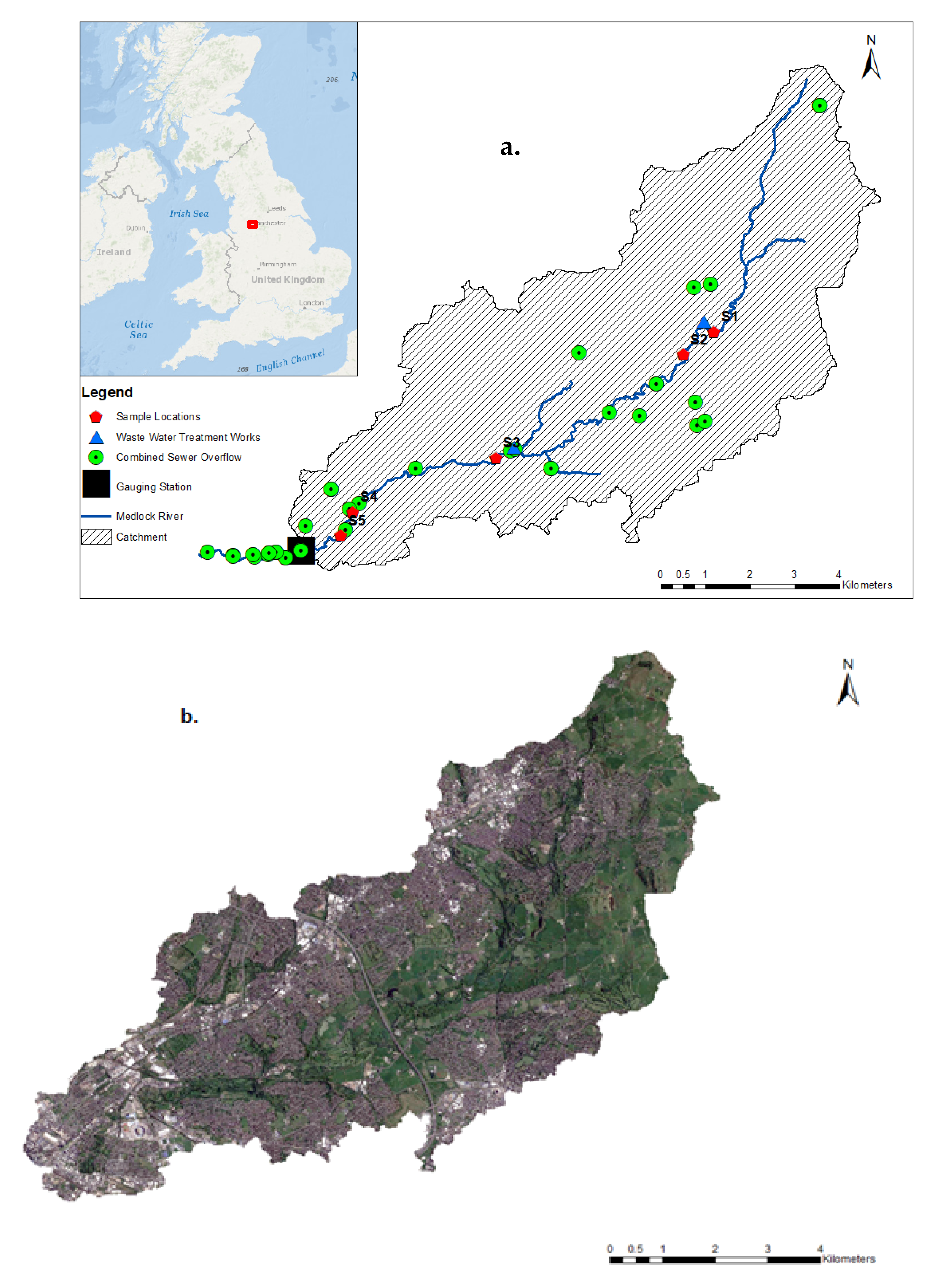
2.1. Study Area: River Medlock

The River Medlock catchment, Figure 1 (a. catchment areas and b. Orthophotomap) has an annual average rainfall of approximately 1025 mm and an average flow rate of 0.883 m³/s (based on the mean monthly flows for the period of record, CEH, 2018). The river rises in the hills of Greater Manchester (National Grid Reference: SD 95308 05431) in North-West England and flows for 22 km through a steep-sided wooded area before it passes through a gauging station (SJ 85781 97858) downstream of the urbanized Manchester City Centre. The region and river has a long industrial history that includes legacy pollution from industrial effluent. Added to this, is a history of inadequately treated sewage [39,40,41,42] and CSO spill events from localized storm events [20,43] and accidental spills (for example, in 2017 a sewage tank leak led to a spill of 21,700 cubic meters of raw sewage, killing fish, see, https://www.bbc.co.uk/news/uk-england-manchester-41160909).
Within the river catchment, there are fifty CSOs, including twenty-nine within the surveyed reach (United Utilities’ personal communication, 2013) as well as numerous surface water drains. The surveyed reach also has a continuously operational WwTW at Failsworth (NGR: SJ 89674 99800). With regard to the CSO discharge points, the main WwTW, and site access, we identified five sampling points (Figure 1a). Sampling site 1 (S1) (NGR: SD 94183 02262) and S2 (NGR: SD 93489 01798) are located upstream of the WwTW and sites S3 (NGR: SJ 89272 99554), S4 (NGR: SJ 86052 98382) and S5 (NGR: SJ 85781 97858) are all located downstream of it. The River Medlock catchment is drained at the gauging station (GS) (NGR: SJ 84900 97518). The number of CSOs which discharge into the sampling sites varies, with seven at S1 and S2, sixteen at S3, five at S4 and one at S5 (United Utilities, personal communication [44]). Characteristics of the five sampling sites are shown on Table 1. Overflow volume data for each sample site was obtained from the water company, United Utilities.

2.2. Water Quality Sampling and Measurement

The Area Ratio (AR) method [45] was used to estimate river discharge (m³/s) at each sampling site. The principal water quality measurements were pH, temperature (°C), conductivity (µS/cm), biochemical oxygen demand (BOD, mg/L), dissolved oxygen (DO, % saturation), suspended solids (SS, mg/L), nitrate-N (NO3-N, mg/L), ammonia-N, phosphate-P (PO4-P, mg/L), ammonia-N (NH3-N), total phosphorus (TP, mg/L), total organic matter (TOM, mg/L), and discharge (m³/s).
A pre-calibrated hand-held multiparameter water quality meter (YSi 556 Multi probe system YSI Incorporated, Yellow Springs, Ohio, USA) was used to take measurements of pH, DO, temperature and conductivity. In a 14-month field campaign between March 2013 to April 2014, monthly spot samples at five sampling sites (S1 to S5) were obtained for the measurement of BOD, SS, TOM, and nutrients. Over the sampling period, a total of 735 samples were collected. These include 70 samples per variable for the analysis of nitrate-N (NO3-N mg/L), phosphate-P (PO4-P), ammonia-N(NH3-N), BOD, SS, conductivity, temperature, pH, DO; TOM (65 samples), and 40 samples for TP. Samples were processed within 24 hours of the sample collection using a SEAL Auto Analyzer 3 High Resolution instrument (SEAL Analytical Ltd, Southampton, UK). Detection limits for phosphate measured as P is 0.004 mg/L and nitrate (measured as N) is 0.05 mg/L. Ammonia-N (NH3-N) concentration (mg/L) was analyzed by spectrophotometry using the Hanna low range reagent kit HI-93700-01 (Hanna Instruments Ltd, Leighton Buzzard, Bedfordshire). The limit of detection for ammonia-N (NH3-N) measured as N is 0.01 mg/L. All chemical variables were analyzed according to the [46].

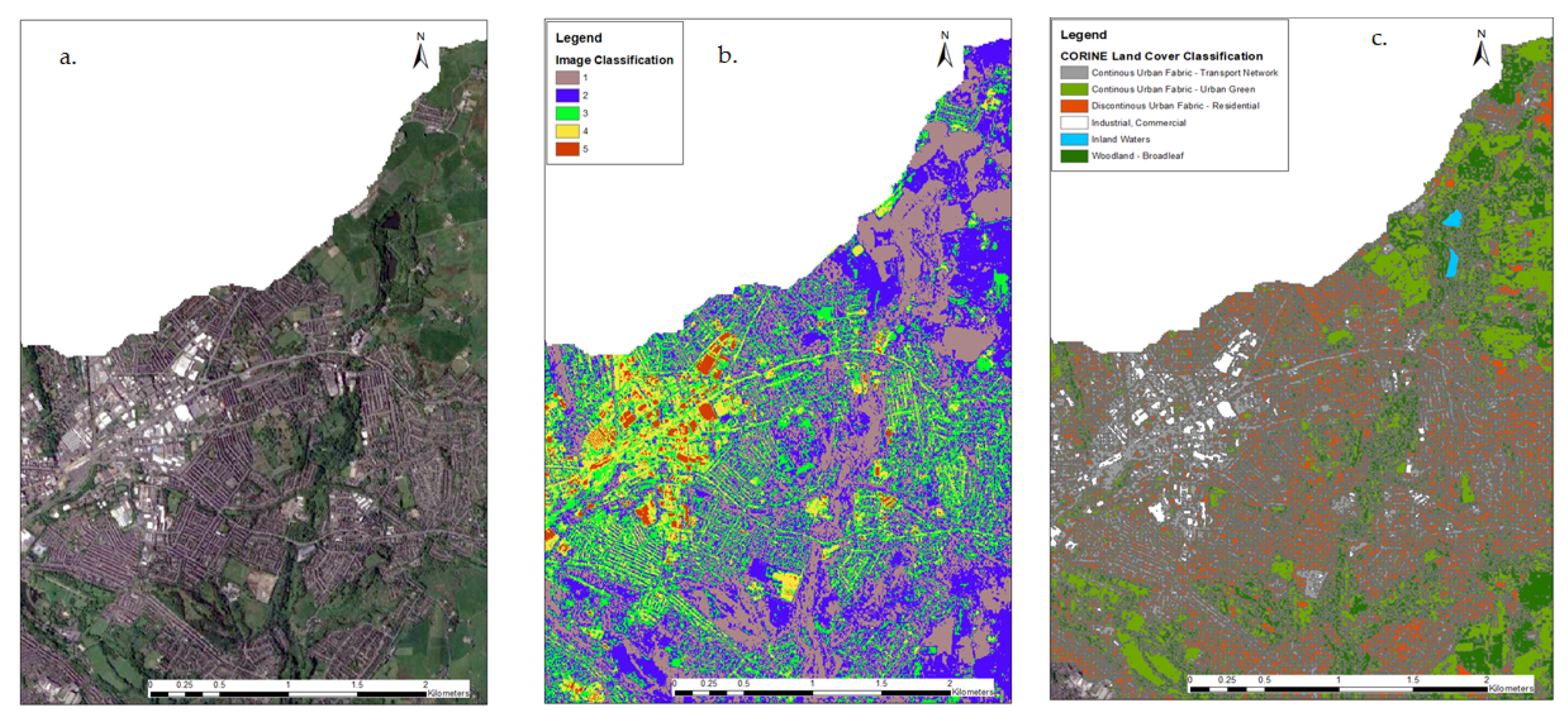
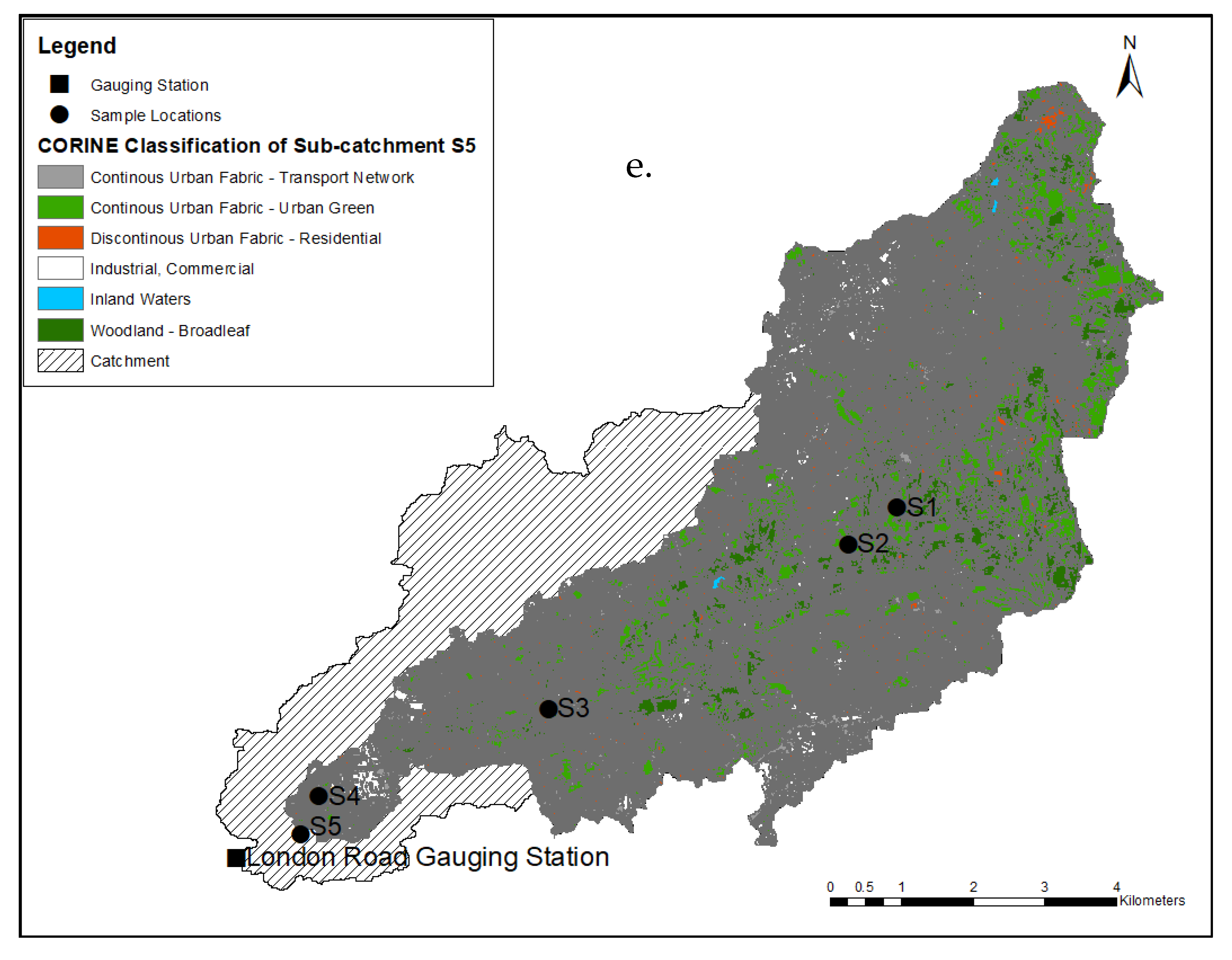
2.3. Classification of Land Cover Patterns

The process used for mapping and determining the spatial distribution of pervious and impervious land cover for the Medlock River catchment was as follows: an orthophotomap of Greater Manchester was generated from Google (Google Maps, 2020. Greater Manchester. Google Maps (online) Available through: University of Manchester (https://www.manchester.ac.uk/) (Accessed 21 February 2020)) satellite imagery with a resolution of 15 cm (Figure 2) was georeferenced (Figure 2a) and the detailed image was classified in ArcGIS 10.4.1 (Figure 2b). The land cover was vectorized (Figure 2c) and further classified according to the CORINE nomenclature [47] into six categories: Continuous Urban Fabric—Transport Networks, Continuous Urban Fabric—Urban Green, Discontinuous Urban Fabric—Residential, Industrial/Commercial, Inland Waters, and Woodland—Broadleaf. The percentage total area of each category was then computed for use in further analyses. The number of pixels (m) recorded for each land cover class was processed for each site and classified by means of their spectral responses.
The land cover map for each pour point (drainage outlet) of the Medlock catchment was determined in relation to catchment area, slope (%) (Figure A1, Appendix A), elevation (mMSL) (Table 1) at a distance of 1 km. Slope was calculated using the ArcGIS Spatial Analyst tool with a DEM (elevation raster) as input. Slope can be measured in percent rise or degrees (with for example 90 degrees representing the slope of a cliff):
S l o p e   ( % ) = r i s e r u n × 100
S l o p e ( ° ) = θ
where
S l o p e   ( ° ) = r i s e r u n   t a n θ

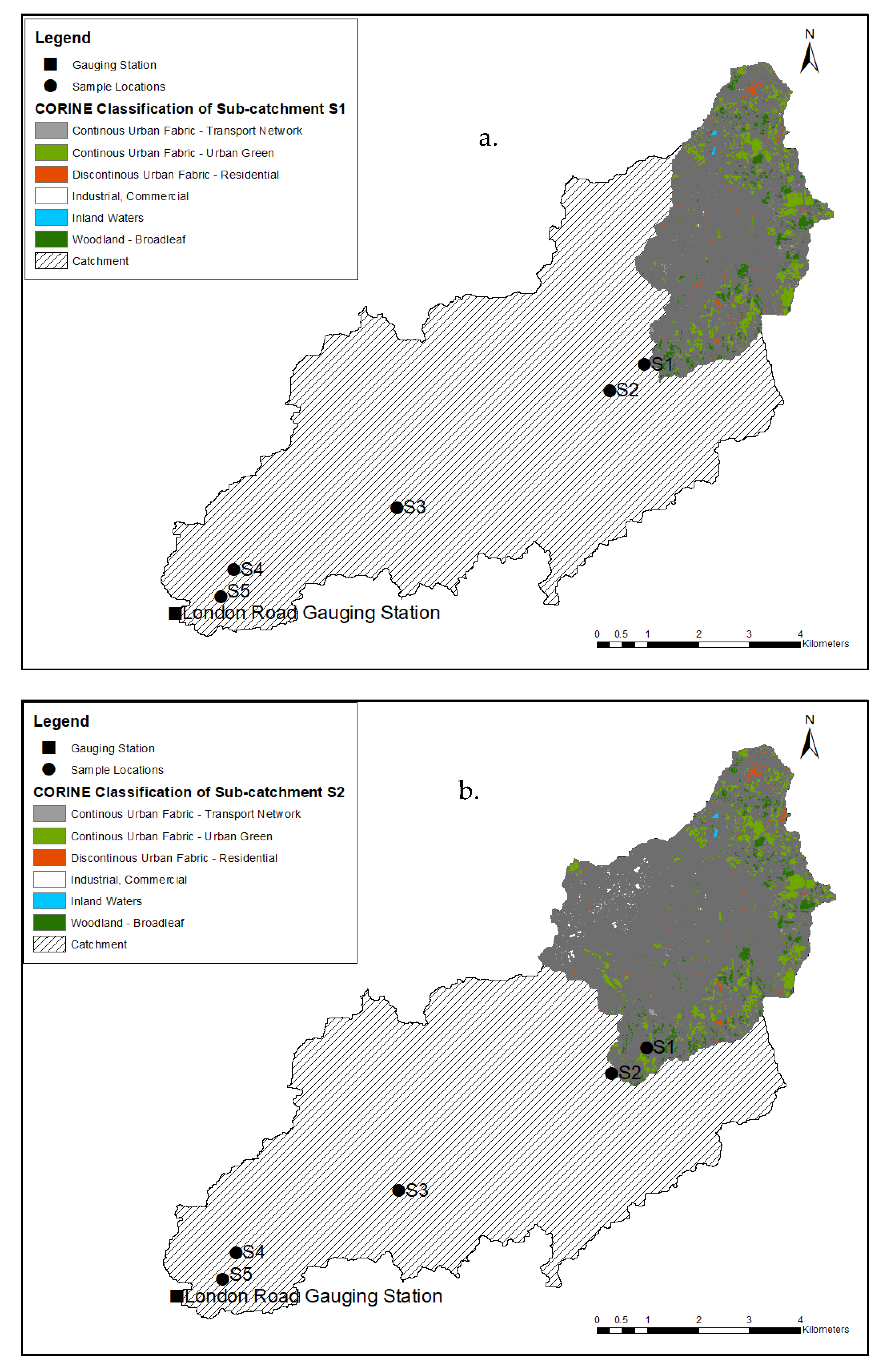
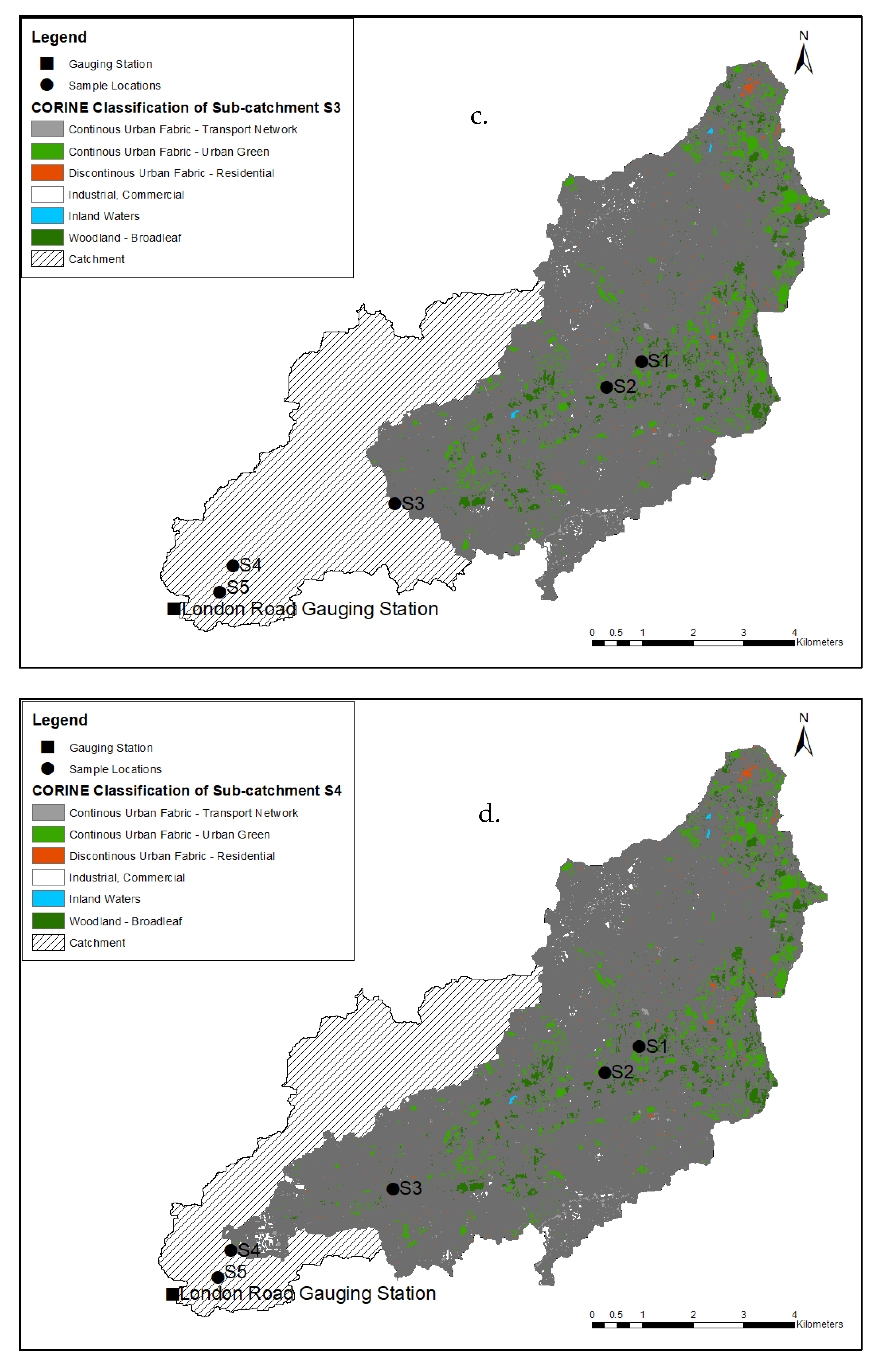
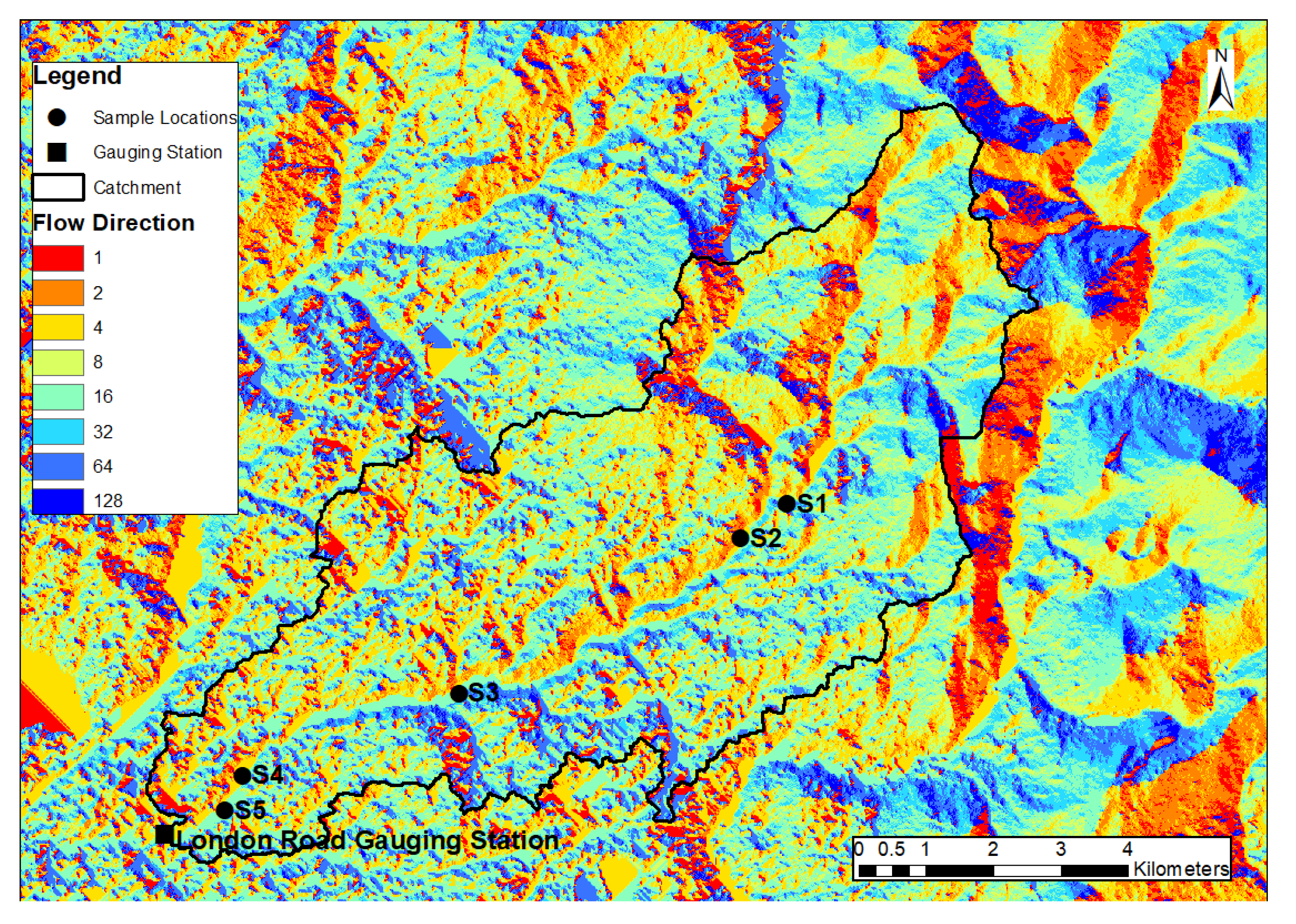
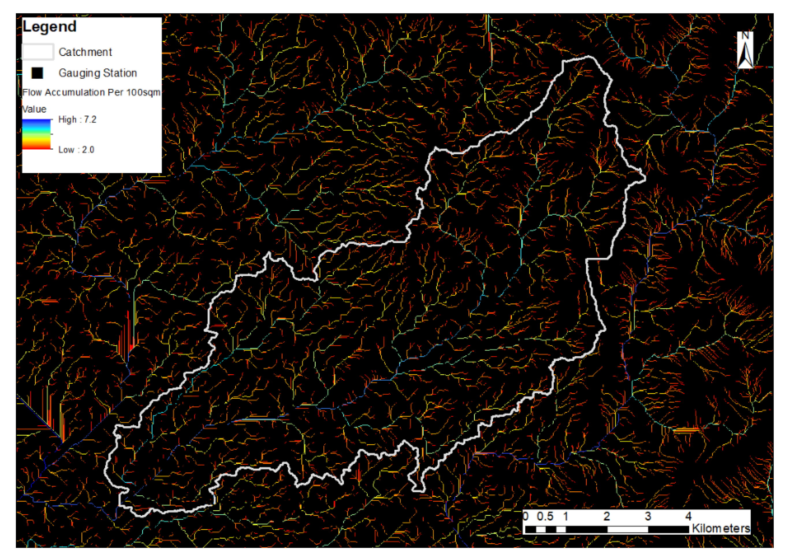
2.4. Drainage Network and Sub-Catchment Delineation

A high-resolution (12.5 m) terrain-corrected DEM was obtained from the ALOS PALSAR (https://earthdata.nasa.gov/eosdis/daacs/asf) dataset and ArcGIS 10.4.1 was used to delineate the drainage networks at the five sample locations. Depression of the DEM data was done with the “fill” tool which ensures there is uniformity in the DEM by filling any holes (or areas of missing data). The “flow direction” was determined with the filled DEM as input. The flow direction grid serves as an input for computing the flow accumulation grid (Figure A2, Appendix A). The “flow accumulation” grid was used to determine the river network to a specific point on the DEM. ArcGIS’s Watershed tool was used to delineate the catchment of the River Medlock (Figure A3, Appendix A). The contributing area to the flow accumulation for each cell ranged from 0 to 423,074 m2. In order to visualize the range of flow accumulation at the sample sites, a threshold of 100 m2 was computed. Pour points and catchment delineation: The pour point is the lowest point (outlet) in the sub-catchment (and the lowest point at the sampling sites) through which water flows under gravity (it is the stream gauge) and delineation takes place upstream of the stream gauge. The point delineation, batch watershed delineation and sub-watershed delineation tools were used in the hydrological analysis-expanding module (Arc Hydro Tools) to divide each sub-catchment either in a diagonal or adjacent pattern. This approach specifies flow directions in the catchment by assigning pixels or cells to one of its eight neighbours, in the flow direction of steepest descent, this is identified as the pour point [31]. This extraction influences the size of the sub-catchment area, location, gradient and range. Thus, the larger the catchment area, the lower the pour point.

2.5. Data Analysis

Using the SPSS Statistics software package version 22.0 Pearson correlation analysis was carried for the physicochemical variables obtained at the sampling points. A stepwise multiple linear regression was applied in order to allow backward selection or removal of variables. The dependent variables were BOD, NO3-N, PO4-P, NH3-N, SS, conductivity, discharge, pH, temperature, TOM, and DO. Correlation between land cover, i.e., compositional attribute (%) and water quality variables were determined. The CORINE land cover nomenclature [47] provides information based on the highest contributing (%) land covers at the spatial scales. The runoff coefficient was determined based on the method of Hvitved-Jacobsen (2010) cross referenced by [5]. That is, the runoff coefficient is found by dividing river discharge at each site by the average precipitation intensity (the annual precipitation (1025 mm)/hr/Area) and drainage area.
All results were compared with the European Union’s Water Framework Directive (EU WFD) standards [48] except for SS, which were compared with the EU’s Freshwater Fisheries Directive. Nitrate standard was determined from the European Commission’s Nitrates Directive.

3. Results

3.1. Sub-Catchment Characteristics of the River Medlock

Maximum elevation in the catchment is 430 m, other characteristics including average slope, catchment area and minimum elevation are shown in Table 1. The size of the catchment area at the GS was calculated at 65.9 km², which is larger than the catchment area reported by the Centre for Ecology & Hydrology (CEH, 57.5 km²). The discrepancy is that the study catchment area takes into consideration other aspects of the sub-catchments not included in the CEH maps.

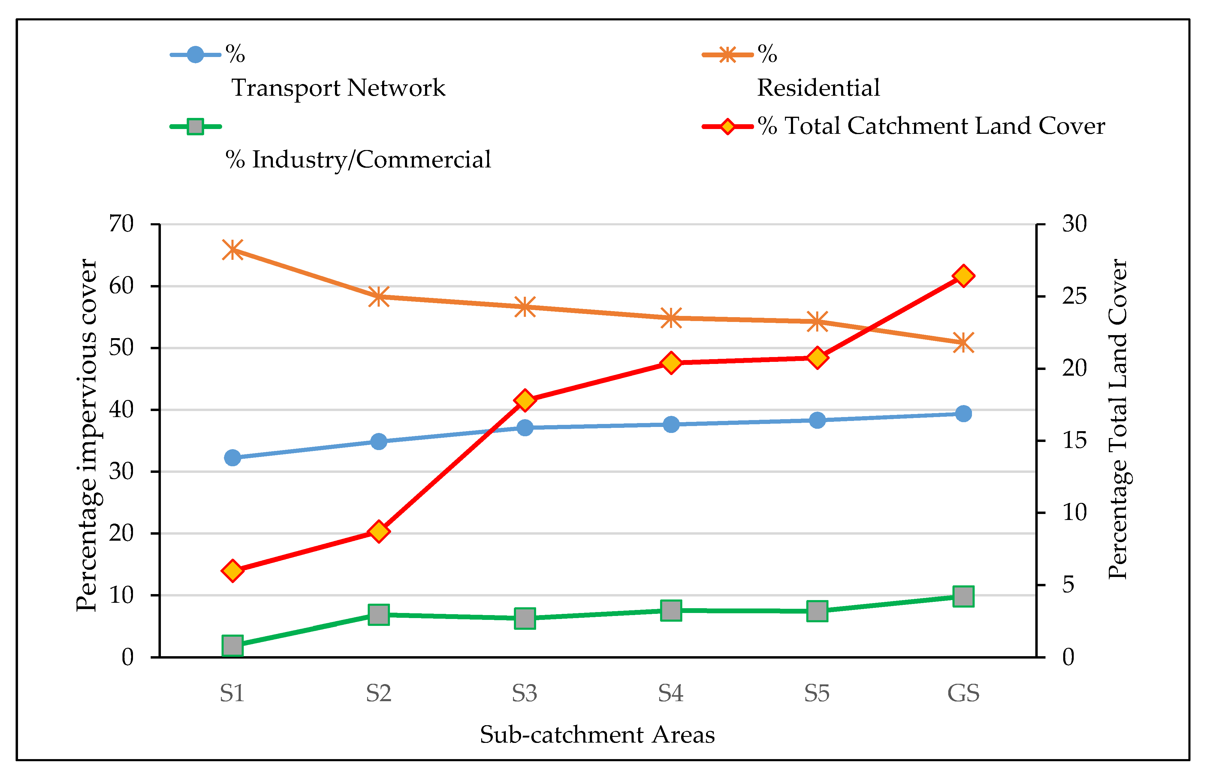
3.2. Land Cover Analysis at the Catchment Level

The distribution of land covers extracted from CORINE for the sampling locations and the GS are shown on Figure 3a–f. These land covers include transport network, residential, industrial, and commercial (now classified as impervious cover); inland water, urban green and woodland (broadleaf). Overall, the percentage of impervious covers increases from S1 to the GS and it is the upland catchment that has the highest percentage of non-impervious land covers.
Table A1 provides information on the land covers by sub-catchment and Table A2 provides more detail on the impervious land covers. The proportion of impervious surfaces is 27% at S1 increasing to 45% at GS. For the catchment as a whole, impervious cover has an area of 98.57 km², i.e., 40% of the total area (Table A1). From Table A1 and Figure 4, the dominant impervious cover in the catchment is the “residential” cover; this is highest at S1, likely reflecting larger property sizes. Residential cover contributes more than 50% at each of the locations. The next dominant cover is the “transport network” which constitutes more than 30% of the impervious cover while the “industrial and commercial” areas contribute less than 10%. The proportion of different types of impervious cover varies between the sites with a generally increasing/decreasing proportion of transport and industrial and commercial/residential moving downstream. Although the runoff coefficient determined from impervious covers of residential and the industrial/commercial per site were insignificant, the runoff coefficient from the transport networks ranged from 1.02 to 4.53. There was a step-change in runoff between sub-catchments S2 and S3 and another large increase between sub-catchment S3 and S4.

3.3. Land Cover Patterns and Water Quality Variables

Table 2 presents the significant correlation coefficients between monthly water quality variables and the percentage land cover. Conductivity correlates negatively with the woodland (broadleaf) and urban green covers but is positively correlated with the impervious covers. Discharge and nutrients correlated positively with the impervious covers and negatively with the urban green covers. SS concentration and TOM had positive correlations with residential cover and urban green cover respectively. DO had positive correlation with Urban Green and woodland (broadleaf cover) and had a negative correlation with the transport network and industry/commercial covers.

3.4. Water Quality Parameters and Standards by Sub-Catchment

Table 3 reports the physicochemical water quality status for the five sampling locations. Note for EU WFD requirements failure in one category results in the failure to meet “good ecological status”. Variables are either classified as “High” which indicates excellent condition, “Very Good”; “Good”; “Moderate”; “Poor” and “Bad”. The levels of pH, temperature, DO and, SS were high indicating excellent water quality while PO4-P, BOD, and NH3-N ranged from poor to very good. For NO3-N, the concentrations were very good. Increasing concentration of conductivity, nutrients, BOD and river discharge were noted at the downstream sections of the river at sites S3, S4, and S5.
Table 4 shows the results of the correlation analysis between the water quality variables. A strong correlation between concentrations of (mg/L) NH3-N and BOD and between NO3-N and PO4-P were recorded at all sample sites. A positive correlation between PO4-P concentration and SS (mg/L) was also recorded at S4. The flux of TP calculated at the WwTW, the upstream S2 and downstream S3 sites, demonstrates that the WwTW contributes TP to the river. The flux at S2 was 0.43 kg TP ha−1 yr−1, 0.94 kg TP ha−1 yr−1 at the WwTW and 0.92 kg TP ha−1 yr−1 at S3.

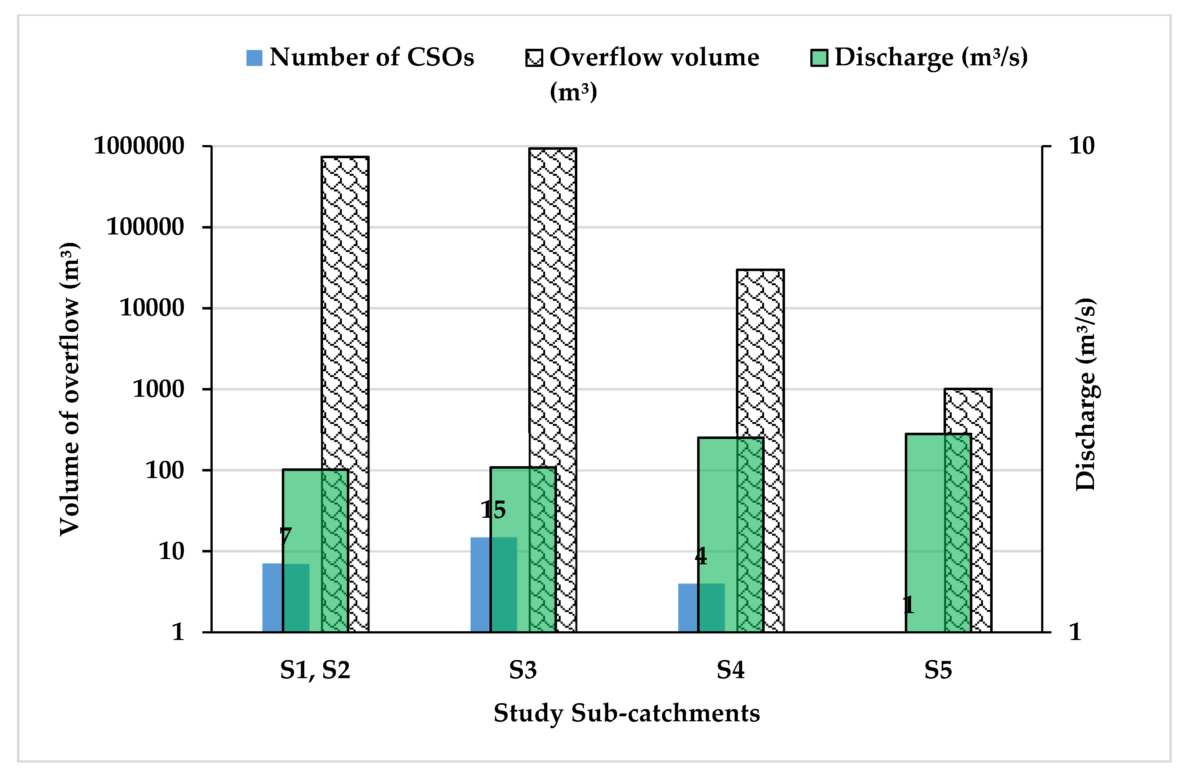
3.5. CSOs: Volume Discharged

Figure 5 shows the volume of CSO versus river discharge across the sample sites. The highest overflowed volume was recorded at S3. At this site, the overflow volume released from 16 operational CSOs was estimated at 932,520 m³. Seven operational CSOs discharge into S1 and S2 with an estimated overflowed volume of 735,617 m³. Overflow volumes were significantly lower at S4 and S5 at 29,902 m³ and 1005 m³, respectively. In 2017, United Utilities categorized CSOs releasing wastewater into sites S1 to S3 as high risk due to the combination of increasing pollution incidents and higher spill volume and frequencies (Utilities, personal communication, 2017). In response to water quality non-compliance at S3, United Utilities is working with the Irwell Catchment Partnership to investigate grey and green infrastructure options to improve water quality.

4. Discussion

4.1. Land Cover and Water Quality

Previous studies have recognized impervious covers as predictors of water quality degradation [1,3,5,12]. Generally, water quality degrades when the percentage of impervious cover is more than 10% [3]. The total area of impervious cover (i.e., transport network, residential, industrial and commercial) in our catchment is 98.57 km² or 40% of the total catchment land cover. Impervious covers by sub-catchment vary between 37%–57% and increases downstream. The predominant impervious land cover is residential buildings which is typical in most urban areas [3]. This complicates the water quality picture as residential areas are sources of SS, P and N pollution and contribute to the overall proportion of impervious surfaces downstream. The industrial legacy in this river catchment [39,40], has been replaced by mixed use impervious land cover (Table A2) that is correlated with high levels of surface runoff, conductivity, and NO3 contaminants and lower DO levels (Figure 4).
Large expanses of impervious surfaces in built-up areas generate higher volumes of overland flow that transport nutrients, SS and other contaminants to artificial drainage networks and rivers [20,23]. We found, impervious covers, in particular transport networks (Table A2) increase runoff, principally from S3 downstream. Following precipitation events, nutrient transfer from impervious areas occurs rapidly [49] transporting contaminants into CSOs and the river, affecting water quality [49]. Table A2 and Figure 3 show that the higher the impervious cover, the lower the river quality (Table 3). Specifically, discharge, conductivity, SS, and nutrients are higher and DO lower at the downstream study sites.
Overall, our study catchment has not met the EU WFD’s good ecological standard due to high PO4-P concentration, which is attributed to discharge from the WwTW and intermittent discharges from CSOs (Figure 5). It is likely difficult to alter the volume of discharge from the WwTW, whereas, the degree of imperviousness in each CSO catchment also determines the conveyance of contaminants into the river [50]. Therefore, the results from the sub-catchment land cover assessment could inform targeted interventions to regulate runoff and improve water quality especially in the highly impervious built up areas, including residential areas. While there are efforts to improve CSO infrastructure and to reduce effluent discharge from point sources, the EA’s Catchment Planning System predicts some improvement as shown in Table A3 (Appendix A) (see https://environment.data.gov.uk/catchment-planning/WaterBody/GB112069061152). However, increased PO4-P concentration in the urban section of the river is forecast to remain Poor and therefore, the implementation of Best Management Practices could be deployed to the river catchment on a case-by-case basis.
Woodland cover can reduce nutrient discharge to rivers, prevent storm water runoff, reduce soil erosion and absorb pollutants. In the study area, the urban green and woodland (Broadleaf) land covers correlated positively with DO and negatively with the nutrients, discharge and conductivity. Yet, in many urban areas, including Greater Manchester, urban woodland has been crowded out by other development. Caution nevertheless should be exercised in the rush to plant trees in catchments for flood risk management or to tackle climate change, as the type of woodland matters, i.e., for this catchment broadleaf woodland might be preferred [2,51].

4.2. Spatial Scales and DEM

Even in a small catchment, where the distance between S2 and S3 is 4.5 km and from S3 and S4 is 3 km, spatial land cover patterns can affect water quality. By selecting a threshold of 100 m2 (Section 2.4) for the delineation of the sub-catchments, the land cover and water quality variables and relationships at the riparian level was revealed. An increased buffer zone, i.e., more than 100 m2 would weaken the influence of the land covers on water quality [25]. River monitoring at different riparian and habitat scales can reveal more information to inform management strategies [26,49].
The variation in catchment size observed in our analysis was attributed to the application of a higher resolution DEM (12.5 m), i.e., 65.9 km² as compared to 57.5 km² determined by the Centre for Ecology and Hydrology UK Integrated Hydrological Digital Terrain Model (IHDTM) on a 50 m grid interval. High resolution DEMs are essential when modelling urban environments, i.e., to predict floods [52,53].
This study demonstrates that ArcGIS and DEM provide useful tools needed to understand the impact of land cover on water quality indicators [54]. Impervious surface covers dominate the river catchment, including transport networks, residential, industrial, and commercial. The WwTW was also shown to be a major contributor to the nutrient loads and the correlation between nutrients, discharge and land covers reflects hydrogeomorphological processes that operate at varying spatial scales [55,56] and measurement scales. Nevertheless, the results of our study may be weakened by the small number of sampling sites. The process of regular sampling and monitoring of urban waterbodies requires permission and access that could be furthered by a more partnership approach to river management.

5. Conclusions

Overall, this study demonstrates that ArcGIS and DEM provide useful tools needed to understand the impact of land cover types and related diffuse source pollutants at the sub-catchment scale on urban water quality. The mix of impervious land covers in each CSO “catchment” determines the composition of overflowed effluent and is a means to separate out this load from the pollutant load discharged from a WwTW. Imperviousness emerged as a potentially useful measure to classify and model river catchments to assess water quality and biodiversity and for flood regulation. Land cover provides an additional target for interventions in river catchments to improve water quality and flow regulation. Interventions could include community and town planning strategies aimed to protect river habitats, through education on garden fertilizer management for households, the development of spatially targeted urban greenspaces, SuDS regulations, or more directly through imperviousness tax on new urban and infrastructural development. The intersection of water quality, urban habitat protection, greenspace for wellbeing, and flood risk management might provide added impetus for integrative management strategies between town planners, regulators, water companies, developers, local community groups and academic researchers.

Author Contributions

The topic was conceptualized by C.M., water quality measurement and analysis by C.M. The development of the maps and the use of the ArcGIS software was analyzed and prepared by K.O.; contributions on different versions of the manuscript discussions on background, policy through partnerships was discussed by R.B. The manuscript was written and data interpreted by C.M. and contributions and editing by R.B. and K.O. All authors have read and agreed to the published version of the manuscript.

Funding

R.B. was funded by the European Union’s Horizon 2020 research and innovation program under the Marie Skłodowska-Curie grant agreement No 659449.

Acknowledgments

Thanks to Andrew Green and Keith White who gave helpful comments to improve the manuscript.

Conflicts of Interest

The authors declare no conflict of interest.

Appendix A

Table A1. Area of the land cover types extracted from the study sub-catchments.
SitesContinuous Urban Fabric–Transport NetworkContinuous Urban Fabric–Urban GreenDiscontinuous Urban Fabric–ResidentialIndustrial, CommercialInland WatersWoodland–BroadleafTotal area (m²) of Land Cover per Sub-CatchmentImpervious Cover %Non-impervious Cover %
S11,302,096.987,093,284.492,661,520.5676,954.1222,569.133,753,243.2014,909,668.4827.1072.90
S22,501,224.479,545,920.154,184,219.37491,579.6522,569.134,974,877.5721,720,390.3433.0466.96
S36,153,087.0018,284,202.329,394,692.581,039,360.6643,686.019,485,514.8044,400,543.3737.3662.64
S47,600,552.8720,420,978.4911,075,106.061,521,639.6143,686.0110,239,830.7950,901,793.8339.6860.32
S57,960,135.5420,648,100.7511,283,991.011,542,921.9843,686.0110,311,191.2651,790,026.5540.1459.86
GS11,718,343.5324,857,706.9315,144,208.772,919,623.1243,686.0111,277,371.0565,960,939.4145.1554.85
Total249,683,361.98
Table A2. Area of the main impervious covers and average runoff coefficient (c); Average runoff coefficient only significant for transport networks. Average precipitation intensity (mm/hr/ha) (I).
SitesContinuous Urban Fabric–Transport Network (Area-(m²); %)Discontinuous Urban Fabric–Residential (Area-(m²); %)Industrial, Commercial (Area-(m²); %)Sum of the Impervious cover (Area-(m²); %)Discharge (m³/s) = QI = Average Precipitation Intensity = mm/h/(m3/s) or ha precipitation = mm) Transp NetwI = Average Precipitation Intensity = mm/hr/ha (precipitation = mm) ResI == Average Precipitation Intensity = mm/hr/ha (precipitation = mm) IC Commercialc–Transp Network = Q/I × A (Transp Networks)
S11,302,096.982,661,520.5676,954.124,040,571.660.158.98 × 10−84.40 × 10−81.52 × 10−61.28
32.2365.871.9
S22,501,224.474,184,219.37491,579.657,177,023.490.238.99 × 10−82.80 × 10−82.38 × 10−71.02
34.8558.36.85
S36,153,087.009,394,692.581,039,360.6616,587,140.240.431.90 × 10−81.25 × 10−81.13 × 10−73.67
37.156.646.27
S47,600,552.8711,075,106.061,521,639.6120,197,298.540.531.54 × 10−81.06 × 10−87.69 × 10−84.53
37.6354.837.53
S57,960,135.5411,283,991.011,542,921.9820,787,048.530.531.47 × 10−81.04 × 10−87.58 × 10−84.53
38.2954.287.42
GS11,718,343.5315,144,208.772,919,623.1229,782,175.420.539.99 × 10−97.73 × 10−94.01 × 10−84.53
39.3550.859.8098,571,257.88
Table A3. EA CPS (2019) Chemical and ecological classification for 2016 and 2027 by reach, where Up = upstream, Down = Downstream. P = Poor, M = Moderate, sG = Supports Good and G = Good. The broad classification of UK waterbodies covers the ecological (biological quality, hydromorphological, physico-chemical, supporting) and chemical (priority substances, hazard substances) statuses. Each element of the classification informs the overall classification status of the waterbody.
Classification Item20162027
UpDownUpDown
Ecological (overall)MMGM
Biological quality elementsPPMM
Hydromorphological supporting elementssGsGsGsG
Physico-chemical quality elementsMMGM
Supporting elements (surface water)MMGG
Chemical (overall)GGGG
Figure A1. The percent slope map for the River Medlock catchment area.
Water 12 00848 g0a1
Figure A2. Flow direction map of the River Medlock catchment. Insert is the D8 legend showing flow direction values increase by a factor of 2 in a clockwise direction of a compass.
Water 12 00848 g0a2
Figure A3. Flow accumulation map of the River Medlock catchment indicates the drainage areas of the sample points (S1–S5) and the gauging station. The flow accumulations were computed over a contributing area of 100 m².
Water 12 00848 g0a3

References

  1. Beck, S.M.; McHale, M.R.; Hess, G.R. Beyond Impervious: Urban Land-Cover Pattern Variation and Implications for Watershed Management. Environ. Manag. 2016, 58, 15–30. [Google Scholar] [CrossRef] [PubMed]
  2. Nisbet, T.; Silgram, M.; Shah, N.; Morrow, K.; Broadmeadow, S. Woodland for Water: Woodland Measures for Meeting Water Framework Directive Objectives; FR(GB-JH) PDF/June11/0099; Forest Research: Surrey, UK, 2011. [Google Scholar]
  3. Arnold, C.L.; Gibbons, C.J. Impervious Surface Coverage: The Emergence of a Key Environmental Indicator. J. Am. Plan. Assoc. 1996, 62, 243–258. [Google Scholar] [CrossRef]
  4. Walsh, C.J.; Roy, A.H.; Feminella, J.W.; Cottingham, P.D.; Groffman, P.M.; Morgan, R.P. The urban stream syndrome: Current knowledge and the search for a cure. J. N. Am. Benthol. Soc. 2005, 24, 706. [Google Scholar] [CrossRef]
  5. Lepeška, T. The Impact of Impervious Surfaces on Ecohydrology and Health in Urban Ecosystems of Banská Bystrica (Slovakia). Soil Water Res. 2016, 11, 29–36. [Google Scholar] [CrossRef] [Green Version]
  6. Zalewski, M. Ecohydrology—The use of ecological and hydrologîcal processes for sustainable management of water resources. J. des Sci. Hydrol. 2003, 47, 823–832. [Google Scholar] [CrossRef] [Green Version]
  7. Chadwick, M.A.; Dobberfuhl, D.R.; Benke, A.C.; Huryn, A.D.; Suberkropp, K.; Thiele, J.E. Urbanization Affects Stream Ecosystem Function by Altering Hydrology, Chemistry, and Biotic Richness. Ecol. Appl. 2010, 16, 1796–1807. [Google Scholar] [CrossRef]
  8. Chin, A. Urban transformation of river landscapes in a global context. Geomorphology 2006, 79, 460–487. [Google Scholar] [CrossRef]
  9. Ding, J.; Jiang, Y.; Liu, Q.; Hou, Z.; Liao, J.; Fu, L.; Peng, Q. Influences of the land use pattern on water quality in low-order streams of the Dongjiang River basin, China: A multi-scale analysis. Sci. Total Environ. 2016, 551–552, 205–216. [Google Scholar] [CrossRef]
  10. Huang, J.; Zhan, J.; Yan, H.; Wu, F.; Deng, X. Evaluation of the impacts of land use on water quality: A case study in the Chaohu lake basin. Sci. World J. 2013, 2013, 7. [Google Scholar] [CrossRef] [Green Version]
  11. Paul, M.J.; Meyer, J.L. Streams in the urban landscape. Annu. Rev. Ecol. Syst. 2001, 32, 333–365. [Google Scholar] [CrossRef]
  12. Walsh, C.J.; Fletcher, T.D.; Vietz, G.J. Variability in stream ecosystem response to urbanization: Unraveling the influences of physiography and urban land and water management. Prog. Phys. Geogr. 2016, 40, 714–731. [Google Scholar] [CrossRef]
  13. Cuffney, T.F.; Mcmahon, G.; Kashuba, R.; May, J.T.; Waite, I.R. Responses of Benthic Macroinvertebrates to Urbanization in Nine Metropolitan Areas. Ecol. Appl. 2010, 20, 1384–1401. [Google Scholar] [CrossRef] [PubMed]
  14. Passerat, J.; Ouattara, K.N.; Mouchel, J.-M.; Rocher, V.; Servais, P. Impact of an intense combined sewer overflow event on the microbiological water quality of the Seine River. Water Res. 2011, 45, 893–903. [Google Scholar] [CrossRef] [PubMed]
  15. Madoux-Humery, A.S.; Dorner, S.; Sauvé, S.; Aboulfadl, K.; Galarneau, M.; Servais, P.; Prévost, M. The effects of combined sewer overflow events on riverine sources of drinking water. Water Res. 2016, 92, 218–227. [Google Scholar] [CrossRef] [PubMed]
  16. Wang, J. Combined Sewer Overflows (CSOs) Impact on Water Quality and Environmental Ecosystem in the Harlem River. J. Environ. Prot. (Irvine Calif.) 2014, 11, 1373–1389. [Google Scholar] [CrossRef] [Green Version]
  17. Xu, Z.; Wu, J.; Li, H.; Chen, Y.; Xu, J.; Xiong, L.; Zhang, J. Characterizing heavy metals in combined sewer overflows and its influence on microbial diversity. Sci. Total Environ. 2018, 625, 1272–1282. [Google Scholar] [CrossRef]
  18. APEM, A. Manchester Ship Canal Strategic Review of Fish; APEM: Heaton Mersey, UK, 2007; p. 139. [Google Scholar]
  19. Myerscough, P.E.; Digman, C.J. Combined Sewer Overflows-Do they have a Future? In Proceedings of the 11th International Conference on Urban Drainage, Edinburgh, Scotland, 31 August–5 September 2008; pp. 1–10. [Google Scholar]
  20. Rees, A.; White, K.N. Impact of Combined Sewer Overflows on the Water-Quality of an Urban Watercourse. Regul. Rivers-Res. Manag. 1993, 8, 83–94. [Google Scholar] [CrossRef]
  21. Committee on Climate Change. UK Climate Change Risk Assessment 2017. Synthesis Report for the Next Five Years; Committee on Climate Change: London, UK, 2016. [Google Scholar]
  22. National Flood Resilience Review. Available online: https://www.gov.uk/government/publications/national-flood-resilience-review (accessed on 16 March 2020).
  23. Thorne, C. Geographies of UK flooding in 2013/4. Geogr. J. 2014, 180, 297–309. [Google Scholar] [CrossRef]
  24. Cheng, P.; Meng, F.; Wang, Y.; Zhang, L.; Yang, Q.; Jiang, M. The impacts of land use patterns on water quality in a trans-boundary river basin in northeast China based on eco-functional regionalization. Int. J. Environ. Res. Public Health 2018, 15, 1872. [Google Scholar] [CrossRef] [Green Version]
  25. Dai, X.; Zhou, Y.; Ma, W.; Zhou, L. Influence of spatial variation in land-use patterns and topography on water quality of the rivers inflowing to Fuxian Lake, a large deep lake in the plateau of southwestern China. Ecol. Eng. 2017, 99, 417–428. [Google Scholar] [CrossRef]
  26. Shi, P.; Zhang, Y.; Li, Z.; Li, P.; Xu, G. Influence of land use and land cover patterns on seasonal water quality at multi-spatial scales. Catena 2017, 151, 182–190. [Google Scholar] [CrossRef]
  27. Xia, L.L.; Liu, R.Z.; Zao, Y.W. Correlation Analysis of Landscape Pattern and Water Quality in Baiyangdian Watershed. Procedia Environ. Sci. 2012, 13, 2188–2196. [Google Scholar] [CrossRef] [Green Version]
  28. Potter, K.M.; Cubbage, F.W.; Blank, G.B.; Schaberg, R.H. A watershed-scale model for predicting nonpoint pollution risk in North Carolina. Environ. Manag. 2004, 34, 62–74. [Google Scholar] [CrossRef] [PubMed]
  29. Buakhao, W.; Kangrang, A. DEM Resolution Impact on the Estimation of the Physical Characteristics of Watersheds by Using SWAT. Adv. Civ. Eng. 2016, 2016, 9. [Google Scholar] [CrossRef] [Green Version]
  30. Lin, Z.; Oguchi, T. Drainage density, slope angle, and relative basin position in Japanese bare lands from high-resolution DEMs. Geomorphology 2004, 63, 159–173. [Google Scholar] [CrossRef]
  31. Jenson, K.S.; Dominigue, O.J. Extracting Topographic Structure from Digital Elevation Data for Geographic Information System Analysis. Photogramm. Eng. Remote Sens. 1988, 54, 1593–1600. [Google Scholar]
  32. Hawker, L.; Bates, P.; Neal, J.; Rougier, J. Perspectives on Digital Elevation Model (DEM) Simulation for Flood Modeling in the Absence of a High-Accuracy Open Access Global DEM. Front. Earth Sci. 2018, 6, 233. [Google Scholar] [CrossRef] [Green Version]
  33. Nigel, R.; Rughooputh, S. Mapping of monthly soil erosion risk of mainland Mauritius and its aggregation with delineated basins. Geomorphology 2010, 114, 101–114. [Google Scholar] [CrossRef]
  34. Wechsler, S.P. Uncertainties associated with digital elevation models for hydrologic applications: A review. Hydrol. Earth Syst. Sci. 2007, 11, 1481–1500. [Google Scholar] [CrossRef] [Green Version]
  35. Wang, G.; Yinglan, A.; Xu, Z.; Zhang, S. The influence of land use patterns on water quality at multiple spatial scales in a river system. Hydrol. Process. 2014, 28, 5259–5272. [Google Scholar] [CrossRef]
  36. Gurnell, A.; Lee, M.; Souch, C. Urban Rivers: Hydrology, Geomorphology, Ecology and Opportunities for Change. Geogr. Compass 2007, 1, 1118–1137. [Google Scholar] [CrossRef]
  37. Whitford, V.; Ennos, A.R.; Handley, J.F. “City form and natural process”—Indicators for the ecological performance of urban areas and their application to Merseyside, UK. Landsc. Urban Plan. 2001, 57, 91–103. [Google Scholar] [CrossRef]
  38. Nolan, P.A.; Guthrie, N. River rehabilitation in an urban environment: Examples from the Mersey Basin, North West England. Aquat. Conserv. Mar. Freshw. Ecosyst. 1998, 8, 685–700. [Google Scholar] [CrossRef]
  39. Burton, L.R. The Mersey Basin: An historical assessment of water quality from an anecdotal perspective. Sci. Total Environ. 2003, 314–316, 53–66. [Google Scholar] [CrossRef]
  40. Douglas, I.; Hodgson, R.; Lawson, N. Industry, environment and health through 200 years in Manchester. Ecol. Econ. 2002, 41, 235–255. [Google Scholar] [CrossRef]
  41. MacKillop, F. Climatic city: Two centuries of urban planning and climate science in Manchester (UK) and its region. Cities 2012, 29, 244–251. [Google Scholar] [CrossRef]
  42. Williams, A.E.; Waterfall, R.J.; White, K.N.; Hendry, K. Manchester Ship Canal and Salford Quays: Industrial legacy and ecological restoration. In Ecological Reviews: Ecology of Industrial Pollution; Cambridge University Press: Cambridge, UK, 2010; pp. 276–308. [Google Scholar]
  43. Blackburn, H.; O’Neill, R.; Rangeley-Wilson, C. Flushed Away: How Sewage is Still Polluting the Rivers of England and Wales; Hydro International: Clevedon, UK, 2017; pp. 1–37. [Google Scholar]
  44. Medupin, C. Spatial and temporal variation of benthic macroinvertebrate communities along an urban river in Greater Manchester, UK. Environ. Monit. Assess. 2020, 192, 84. [Google Scholar] [CrossRef] [Green Version]
  45. Archfield, S.A.; Vogel, R.M. Map correlation method: Selection of a reference streamgage to estimate daily streamflow at ungauged catchments. Water Resour. Res. 2010, 46, 1–15. [Google Scholar] [CrossRef]
  46. Environment Agency-Standing Committee of Analysts (SCA library): Methods for the Examination of Waters and Associated Material—Index of Methods for the Examination of Waters and Associated Materials 1976–2011 Blue Book 236. 2011. Available online: http://www.standingcommitteeofanalysts.co.uk (accessed on 15 March 2020).
  47. Barbara, K.; György, B.; Gerard, H.; Stephan, A. Updated CLC Illustrated Nomenclature Guidelines; European Environment Agency: Copenhagen, Denmark, 2017; pp. 1–124. [Google Scholar]
  48. WFD_UKTAG (2013) UKTAG WFD Environmental Standards River Basin Management 2015–2021. November 2013. Available online: http://www.wfduk.org/sites/default/files/Media/Environmental%20standards/UKTAG%20Environmental%20Standards%20Phase%203%20Final%20Report%2004112013.pdf (accessed on 15 March 2020).
  49. Luo, K.; Hu, X.; He, Q.; Wu, Z.; Cheng, H.; Hu, Z.; Mazumder, A. Impacts of rapid urbanization on the water quality and macroinvertebrate communities of streams: A case study in Liangjiang New Area, China. Sci. Total Environ. 2018, 621, 1601–1614. [Google Scholar] [CrossRef]
  50. Klein, R.D. Urbanization and Stream Quality Impairment. Water Resour. Bull. 1979, 15, 948–963. [Google Scholar] [CrossRef]
  51. Gagkas, Z.; Heal, K.; Stuart, N.; Nisbet, T.R. Forests and Water Guidelines: Broadleaf Woodlands and the Protection of Freshwaters in Acid-Sensitive Catchments. In Proceedings of the BHS 9th National Hydrology Symposium, Durham, England, 11–13 September 2006; pp. 53–58. [Google Scholar]
  52. Savage, J.T.S.; Bates, P.; Freer, J.; Neal, J.; Aronica, G. When does spatial resolution become spurious in probabilistic flood inundation predictions? Hydrol. Process. 2016, 30, 2014–2032. [Google Scholar] [CrossRef] [Green Version]
  53. Fewtrell, T.J.; Bates, P.D.; Horritt, M.; Hunter, N.M. Evaluating the effect of scale in flood inundation modelling in urban environments. Hydrol. Process. 2008, 22, 5107–5118. [Google Scholar] [CrossRef]
  54. Flaherty, D.J.; Drelich, J. The Use of Grasslands to Improve Water Quality in the New York City Watershed; Session 27—Integration of Environmental and Agricultural Policy; European Environment Agency: Copenhagen, Denmark, 1996. [Google Scholar]
  55. Grabowski, R.C.; Surian, N.; Gurnell, A.M. Characterizing geomorphological change to support sustainable river restoration and management. Wiley Interdiscip. Rev. Water 2014, 1, 483–512. [Google Scholar] [CrossRef]
  56. Gurnell, A.M.; Rinaldi, M.; Belletti, B.; Bizzi, S.; Blamauer, B.; Braca, G.; Buijse, A.D.; Bussettini, M.; Camenen, B.; Comiti, F.; et al. A multi-scale hierarchical framework for developing understanding of river behaviour to support river management. Aquat. Sci. 2016, 78, 1–16. [Google Scholar] [CrossRef] [Green Version]
Figure 1. River Medlock catchment area and the study sites. Insert is the location of the river in Greater Manchester, UK (a); Orthophotomap of the river catchment (b).
Water 12 00848 g001
Figure 2. Georeferenced map of the River Medlock (a); Detailed orthophotomap classified in ArcGIS 10.4.1 (b); Vectorized land cover (c).
Water 12 00848 g002
Figure 3. CORINE land cover patterns at sub-catchments S1 to S5 (ae) and the Gauging Station (f).
Water 12 00848 g003aWater 12 00848 g003bWater 12 00848 g003cWater 12 00848 g003d
Figure 4. The percent total land cover verses impervious cover for transport networks, industry/commercial and residential. Percentage total land cover found to increase downstream of the catchment.
Water 12 00848 g004
Figure 5. Volume (Log10) (m³) of wastewater and discharge (Log10) (m³/s) released from combined sewer overflow (CSO) for each sample site.
Water 12 00848 g005
Table 1. Catchment characteristics including the sub-catchment sampling sites S1–S5 and GS obtained from the digital elevation model (DEM).
Sub-CatchmentGrid Reference LatitudeLongitudeDistance (km from Source)Average Slope (%)Sample Point Catchment Area (km²)Elevation (Mean Sea Level)
S1SD 94183 0229553.5173−2.08926.610.7213.65182
S2SD 93489 0179853.5128−2.09968.59.4520.55159
S3SJ 89272 9955453.4925−2.1631137.5643.98114
S4SJ 86052 9838253.4819−2.211616.17.2450.1693
S5SJ 85781 9785853.4772−2.215717.47.2150.8590
GSSJ 84800 9750053.4740−2.2305186.5765.9489
Table 2. Significant correlations between water quality variables and land cover, Number of sampling sites = 5, r = correlation coefficient.
Land Cover and Water Quality Variablesrp
Transport Network
DO mg/L−0.9370.019 *
Conductivity0.9910.001 *
TOM mg/L−0.8850.046 *
Discharge m³/s0.9640.008 **
NO3-N mg/L0.9040.035 *
Urban Green
DO mg/L0.9340.020 *
Conductivity−0.9910.001 *
TOM mg/L0.9040.035 *
Discharge m³/s−0.9620.009 **
PO4-P mg/L−0.8810.049 *
NO3-N mg/L−0.9130.031 *
Residential
Conductivity0.9930.001 **
Suspended solids mg/L0.9040.035 *
Discharge m³/s1.0000.000 **
PO4-P mg/L0.9080.033 *
NO3-N mg/L0.9590.001 *
Industrial/Commercial
DO mg/L−0.8970.039 *
Conductivity0.9280.023 *
Discharge m³/s0.9150.029 *
Woodland (broadleaf)
DO mg/L0.8990.038 *
Conductivity µS/cm−0.9990.000 **
** Correlation is significant at the 1% and at the * 5% level (2-tailed).
Table 3. Water quality measurements by sample site and EU Directives. The median values for all variables were determined except for SS where the mean values were provided to align with classification. Number of samples per site per variable S1 = 14, S2 to S5 = 15 each. All variables compared with EU Water Framework Directive (EU WFD) except suspended solids (mg/L) compared with the * Freshwater Fisheries Directives and ** Nitrates Directive and Drinking Water Directive applied to NO3-N (mg/L).
VariablesSub-Catchment AreasMedian % PercentileStandards
EU WFD,
* Freshwater Fisheries Directive
** Nitrates Directive and Drinking Water Directive
Interpretation
Temperature
(°C) 2% and 98% percentile
S19.85–15.3≤20High
S29.55.1–14.8
S310.45.4–17.7
S410.24.9–17.3
S510.34.8–18.5
pH 5% and 10th percentileS17.8587.40–7.46≤6–9High
S27.797.50–7.61
S38.0057.74–7.77
S48.047.80–7.81
S58.067.83–7.86
DO (% sat)
10%–90th percentile
S1103.797.94–115.5≥70%High
S210185.8–111.6
S3101.594.81–117.2
S4100.993.82–113.7
S599.582.04–113.9
* Suspended solids (mg L−1)
Freshwater Fisheries Directive
S14.183 <25High
S26.029
S311.59
S415.03
S512.05
NH3-N (mg L−1)
1%–99th percentile
S10.350–2.480.04Poor
S20.40–2.18
S30.590–2.50
S40.40.01–2.18
S50.430–2.55
BOD(mg L−1)
1%–99th percentile
S11.520–13.68≤14Good to Moderate
S21.980–13.1≤14Good to Moderate
S320.04–14.92≤19Good to Moderate
S42.60.55–16.13≤19Good to Moderate
S52.490–5.1≤19Very Good
TOM (mg L−1)
1%–99th percentile
S10.010–28.13
S20.010–25.93
S30.840–18.81
S40.330–14.04
S50.670–17.75
** NO3-N (mg L−1)
(5%–95%) Nitrate Directive
S19.720.14–4.9850Very Good
S29.600.14–4.4650Very Good
S310.70.59–11.6850Very Good
S410.30.611–9.6050Very Good
S510.340.523–9.2350Very Good
PO4-P (mg L−1)
(5%–95%)
S10.0230–0.580.215–1.098Very Good
S20.0270–1.010.215–1.099Very Good
S30.4620.03–1.610.215–1.100Moderately Poor
S40.4440.02–1.250.215–1.101Moderately Poor
S50.4470.02–1.250.215–1.102Moderately Poor
Table 4. Significant correlations between analyzed physicochemical variables by sample point. N = number of samples S1= 22; S3–S5 = 23 each.
Sites/Parameterspr
S1
BOD (mg/L) /NH3-N (mg/L)00.729 ***
Conductivity (µS/cm)/pH0.016−0.517 **
NO3-N (mg/L)/PO4-P (mg/L)0.0010.652 ***
Q (m³/s)/NO3-N (mg/L)0.0130.509 **
S2
BOD (mg/L)/NH3-N (mg/L)0.0010.639 ***
Q(m³/s)/NO3-N (kg/d)0.0190.485 **
S3
BOD (mg/L)/NH3-N (mg/L)0.0180.501 **
NO3-N (mg/L)/PO4-P (mg/L)00.797 ***
S4
BOD (mg/L)/NH3-N (mg/L)0.0090.535 ***
NO3-N (mg/L)/PO4-P (mg/L)00.797 ***
PO4-P (mg/L)/SS (mg/L)0.020.481 **
S5
NO3-N (mg/L)/PO4-P (mg/L)00.838 ***
*** Correlation is significant at 1% level and ** at the 5% level (2-tailed).

