Article

Lidar and Ceilometer Observations and Comparisons of Atmospheric Cloud Structure at Nagqu of Tibetan Plateau in 2014 Summer

1
Ocean Remote Sensing Institute, Ocean University of China, Qingdao 266100, China
2
Laboratory for Regional Oceanography and Numerical Modeling, Qingdao National Laboratory for Marine Science and Technology, Qingdao 266100, China
3
State Key Laboratory of Science Weather, Chinese Academy of Meteorological Science, Beijing 100081, China
*
Author to whom correspondence should be addressed.
Atmosphere 2017, 8(1), 9; https://doi.org/10.3390/atmos8010009
Submission received: 12 September 2016 / Revised: 29 November 2016 / Accepted: 5 December 2016 / Published: 17 January 2017

Abstract

:
In the project of the Third Tibetan Plateau Experiment of Atmospheric Science (TIPEX III), the intensive observation of cloud and precipitation in Nagqu was conducted from 1 July to 31 August 2014. The CL31 ceilometer and a WAter vapor, Cloud and Aerosol Lidar (WACAL) were deployed and focused on studying the cloud macroscopic characteristics and vertical distribution. The statistical result of CL31 ceilometer in continuous operation mode shows that the cloud occurrence is about 81% with a majority of simple one-layer cloud. The cloud base and top height are retrieved by improved differential zero-crossing method using lidar data. The results of cloud base height (CBH) are compared with CL31 ceilometer, showing a good consistency with each other, however, in some cases, the CL31 ceilometer overestimates the CBH and is also validated by synchronous radiosonde data. The time snippet comparisons of cloud property between CL31 ceilometer and lidar imply that the cloud properties have obvious diurnal variations with “U” shape distribution. The cloud development including the time-spatial distribution features also has distinct diurnal variations based on the lidar measurement. The detection range of lidar goes beyond the maximum height of CL31 ceilometer, offering substantial observations to the analysis of cirrus cloud radiation characteristics and formation mechanism.

1. Introduction

Clouds play a vital role in the radiative transfer within the Earth’s atmosphere surface system and thus for climate system [1,2]. Different types of cloud have varying effects on the atmosphere. Generally, clouds exert both a cooling effect on the surface by reflecting shortwave radiation back into space and a warming effect by trapping longwave radiation emitted from the Earth’s surface [3,4,5,6]. Due to its complex climate feedback and uncertainty in the process of climate change, the study of cloud macroscopic properties, such as cloud type, cloud base and top height, and temporal and spatial distributions in high temporal and spatial resolution are significant for describing the impact of clouds in a changing climate.
The Tibetan Plateau is a vast elevated plateau in the middle of the Eurasian continent with averaged elevation above 4500 m mean sea level (m.s.l.). It has an important role in the global and regional climate system by its unique dynamic and thermodynamic forcing effect [7,8], and the thorough research on cloud distribution is quite essential for understanding the climate of Asian monsoon region and Tibetan Plateau. With the development of remote sensing, satellite data have been applied to the Tibetan Plateau cloud characteristics research. Wang et al. [9] analyzed the Tibetan Plateau cloud occurrence, vertical distribution and its seasonal variation using CloudSat/Cloud-Aerosol Lidar and Infrared Pathfinder Satellite Observations (CALIPSO) data, and found that thin cloud with a range of 4–11 km are most frequent in this area and a higher grid vertical resolution of GCM is needed for accurate description of cloud occurrence and location. Zhao et al. [10] analyzed the distribution of Tibetan Plateau cloud total water path (TWP) and its seasonal variation using CloudSat data, finding that the value of TWP in warm season is larger than cool season’s and the vertical distribution of precipitation clouds in Tibetan Plateau is quite different from East Asia’s. Fu et al. [11] analyzed a case study of the precipitation cloud in the valley of Tibetan Plateau, indicating that the topographic forcing is the main factor of this cloud formation. However, the deficiency of ground-based observation is the main constraint for the accurate retrieval using satellite data. Recently, lidar has been an effective quantitative tool of ground-based cloud detection due to its high temporal-spatial resolution and measurement accuracy [12]. Liu et al. [13] carried out the research on microphysical and macroscopic features of cloud and precipitation vertical distribution using multiple wavelength radar and lidar devices during TIPEX III, and found that the statistics parameters of cloud have obvious diurnal variations. He et al. [14] analyzed the cirrus cloud geometry and optical characteristics in summer Tibetan Plateau using micro-pulsed lidar, finding that there exists obvious difference between Tibetan Plateau and same latitude area. Liu [15] analyzed the aerosol optical characteristics in Nagqu using micro-pulsed lidar, and indicated that Nagqu area has a better air quality than other areas’ in China.
As a part of the TIPEX III, the Ocean University of China (OUC) operated the CL31 ceilometer (short for CL31) and the WACAL in summer of 2014 to carry out the research on the microphysical characteristics and the vertical structure of cloud in Tibetan Plateau. In this paper, the cloud characteristics based on CL31 observation is firstly analyzed. Then, the comparison of the CBH between CL31 and the WACAL is carried out. The time snippet comparison of CBH and the cloud occurrence between these two devices is analyzed after the determination of the data acquirability of the WACAL. Finally, the averaged spatial distribution of different layer clouds measured by the WACAL is analyzed at different observation periods, further making up the constraint of CL31 undetectable condition above 7.5 km.

2. Data and Methodology

Lidar observations in summer of 2014 as a part of the TIPEX III were performed at the Nagqu Meteorological Bureau (31.48° N, 92.06° E, 4508 m m.s.l.) on the Tibetan Plateau. The location of the Nagqu site and the topography of the Tibetan Plateau are shown in Figure 1. Nagqu is located in the central part of the Tibetan Plateau. The elevated surface heat and the rising air over the plateau lead to anticyclonic circulation and divergence in the upper troposphere and lower stratosphere [16].

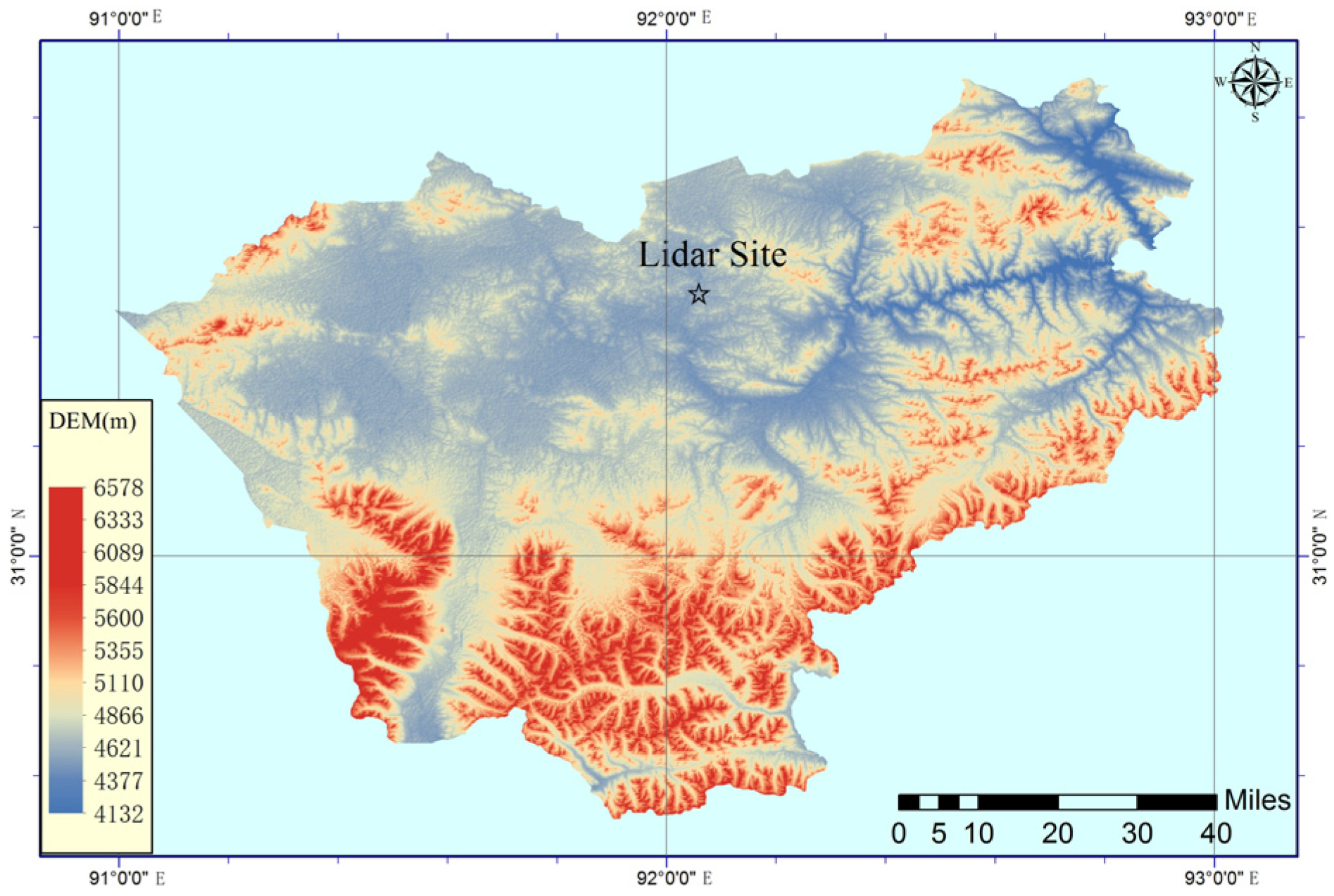
2.1. Set Up Introduction
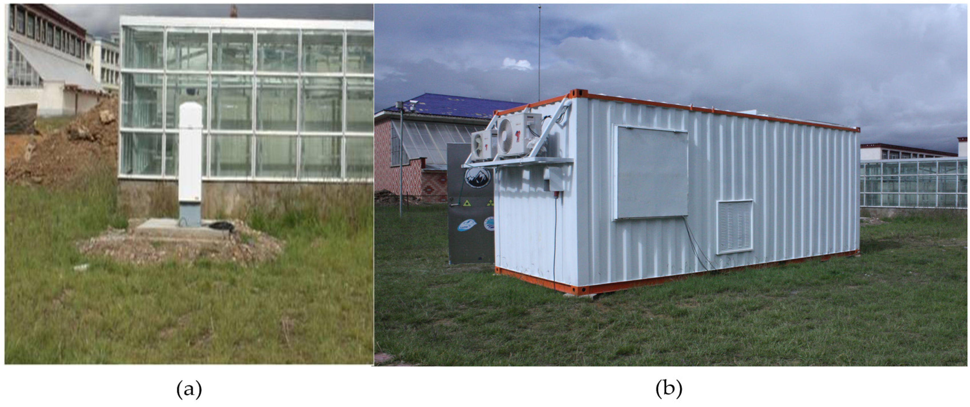
2.1.1. CL31

The CL31 measures backscattered light at wavelength of 910 nm with measurement ranging from 0 to 7.6 km. The minimum vertical and temporal resolutions are 5 m in height and 2 s in time, respectively. The time resolution used in this study amounts to 16 s. The CL31 can detect three cloud layers simultaneously with a pulsed diode laser lidar technology. The single-lens technology provides excellent performance at low altitudes and reliable operation in all weather. Furthermore, fast measurement also provides reliable detection of thin cloud layers below a solid cloud base. Figure 2a shows the photo of CL31. The basic parameters of CL31 are listed in the left of Table 1 [17].

2.1.2. WACAL

The lidar measurements are conducted with the fully automatic portable multi-wavelength Raman and polarization lidar WACAL [18] by Ocean University of China (OUC). Figure 2b shows the photo of WACAL, and the basic parameters are listed in the right of Table 1. WACAL measures backscattered light at wavelength of 355 nm, 532 nm and 1064 nm and Raman scattered light at 387 nm and 407 nm. For cloud measurement, the 532 nm channel with pulse energy of 120 mJ is used. The beam expander is used to decrease the beam divergence angle and ensure the high optical transmittance. After a laser pulse is transmitted into the atmosphere, the backscattered signal is collected by telescope and then transmitted to the detection system. The 532 nm signal is separated by the dichroic long-pass filter, and then the 532 nm parallel-polarized and perpendicular-polarized signals are separated by the polarizing beam splitter (PBS) and detected by photomultiplier tubes (PMTs) to retrieve the depolarization ratio. The sum of parallel-polarized and perpendicular-polarized signals is used to study cloud structure. The vertical and temporal resolutions are 3.75 m in height and 30 s in time, respectively. In contrast to CL31, the more powerful laser of WACAL enables measurements up to 15 km, offering substantial observations to the analysis of high cloud.

2.1.3. Model GTS1 Digital Radiosonde

In operation with Model GFE (L) 1 Secondary Radar, Model GTS1 digital radiosonde can measure the atmospheric temperature, pressure, relative humidity, wind direction and wind velocity from ground up to altitude of 30 km. The Radar captures and automatically tracks signals transmitted from a radiosonde attached to a balloon to obtain atmospheric conditions, calculating wind direction and wind velocity while the balloon is being uplifted, and it inputs the received data along with angle data and time signal into the data processing unit for real time data processing. GTS1 has come into use in some upper air stations as the new generation upper air sounding in China because of its high sampling rate, high anti-jamming capability, modularity and digitization characteristics. The basic parameters of GTS1 digital radiosonde are listed in Table 2 [19].

2.2. Methodology

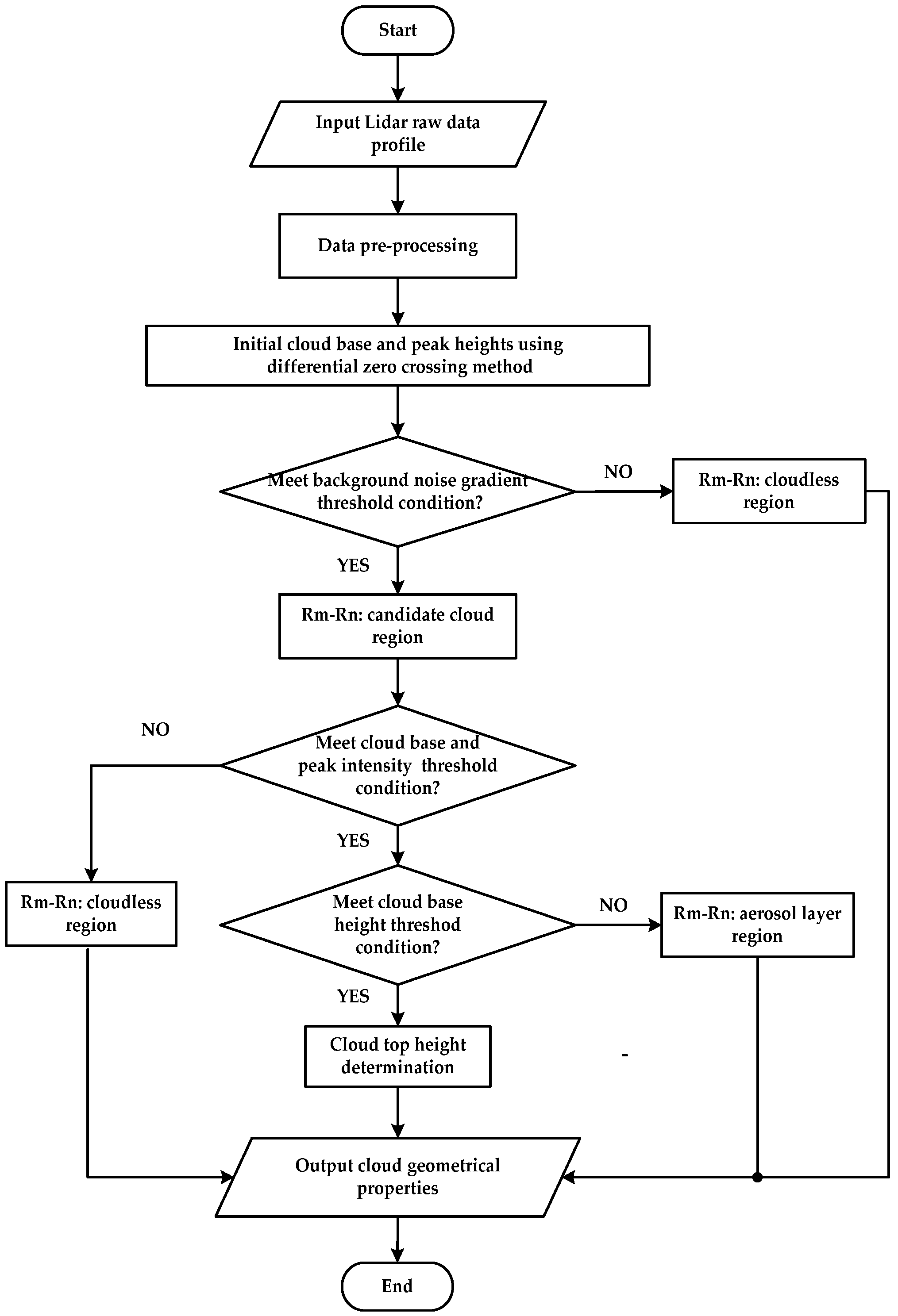
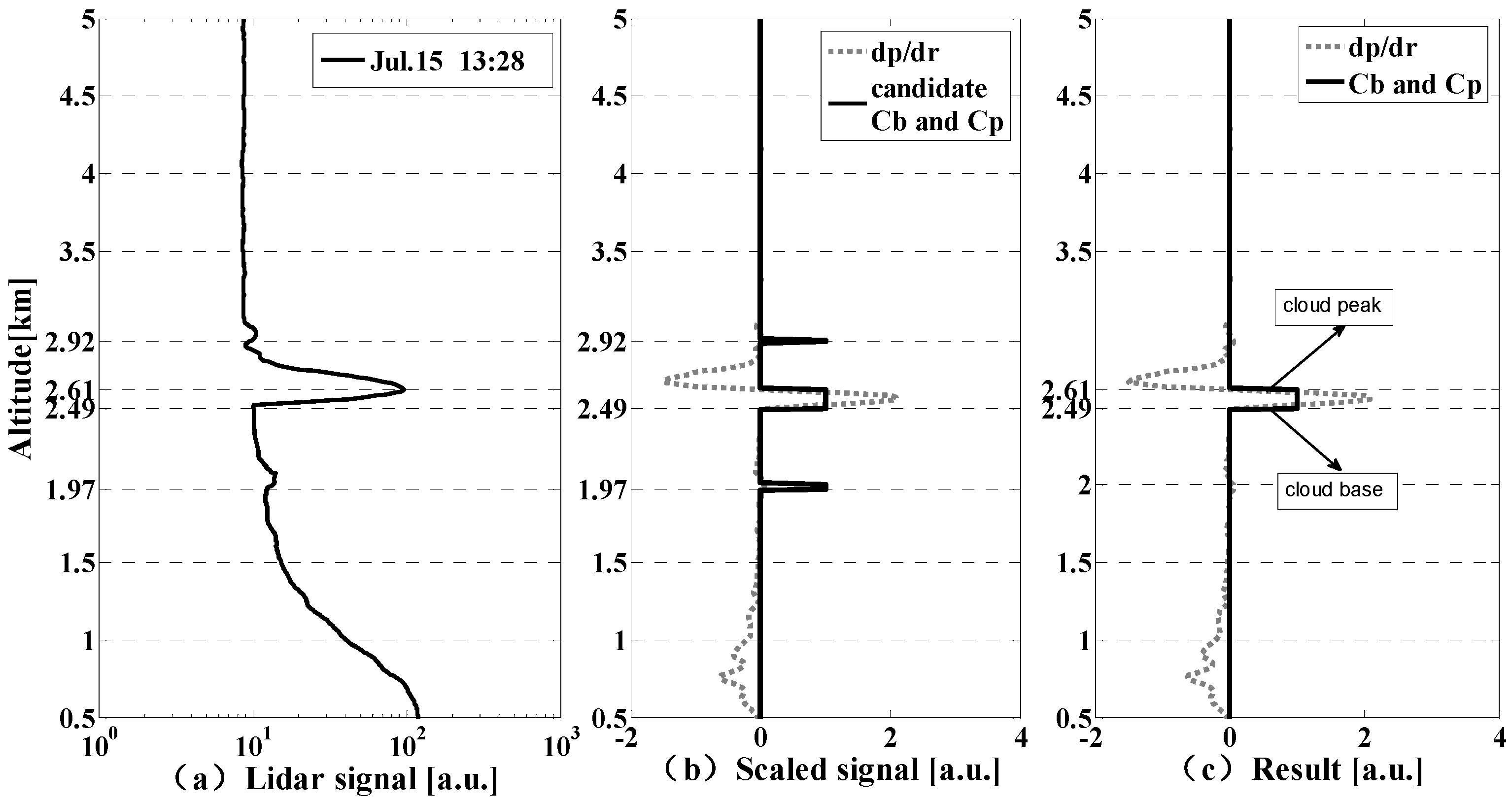
2.2.1. Improved Differential Zero-Crossing Method Using WACAL

The methods of CBH retrieval using lidar data mainly include the threshold method [20] and differential zero-crossing method [21]. In threshold method, the CBH is defined as the level where there is firstly an increase in signal above the clear background level and of a magnitude equal to N times the standard deviation of the background fluctuations Furthermore, it is required that the signal should be increased continuously for at least M successive height intervals. Thus, it has a relative complex adjustment process since the threshold value M and N need to be adjusted repeatedly based on the properties of cloud and aerosol so that it is hard to realize the automatic processing. The differential zero-crossing method judges the point where the value of the first derivative of the lidar backscatter power changes from negative to positive as the CBH, but there may exist misjudgment when the Signal Noise Ratio (SNR) is lower or the fluctuation of noise is too large. In this section, the improved differential zero-crossing method is used [22], and it is based on differential zero-crossing method, and additionally three threshold conditions are also used to effectively avoid misdiagnoses. Figure 3 shows the flow chart of cloud properties retrieval based on improved differential zero-crossing method. The raw lidar data need pre-processing including the noise removal and temporal-spatial average to improve their SNR. In order to decrease the cloud layer misdiagnoses due to the aerosol layer and background noise, three threshold conditions are carried out in this algorithm. Firstly, the background noise gradient threshold is calculated. Specifically, the mean value K and the standard deviation e of the background noise first derivative are calculated, and the candidate cloud region should meet the condition of dP ( r ) / dr K + ne , where P ( r ) is the lidar signal after data pre-processing, and n is a positive value with fine tuning in different atmospheric conditions, otherwise, the analyzed area is regarded as cloudless area. Secondly, the threshold of cloud base and peak intensity should be calculated. Specifically, the mean value M of the background noise is calculated, and the candidate cloud region should be satisfied that the lidar signal intensity difference between the cloud peak P peak ( r ) and cloud base P base ( r ) is larger than aM , that is, P peak ( r ) - P base ( r ) aM , and a is a positive value with fine tuning in different atmospheric conditions, the tuning standard of which has been listed in Table 3. Otherwise, the analyzed area is regarded as cloudless area. Thirdly, the threshold of CBH is determined based on the ground-based observations that the averaged low CBH is about 512 ± 148 m with the lidar overlap into consideration. Thus, the layer below 500 m above ground level (AGL) is eliminated [23]. Figure 4 shows the case study using improved differential zero-crossing method [22]. The left diagram is lidar signal, the middle diagram is the first derivative of the lidar signal (dashed line) with candidate cloud layer (solid line value equals to 1). Since the amplitude difference of the first derivative of lidar signal induced by cloud, aerosol and background noise is significant in most cases, the final cloud layers shown in the right diagram are selected using three threshold conditions mentioned above. After the determination of CBH, the cloud top height is determined where the lidar signal is less than the cloud base’s and | dP ( r ) / d r | K + n e . When the cloud is optical thick and impenetrable, the point with a minimum value above the cloud peak height in the candidate area is regarded as the cloud top height. It is noted that comparison and combination in adjacent cloud layers should be done when the cloud has complex structure.

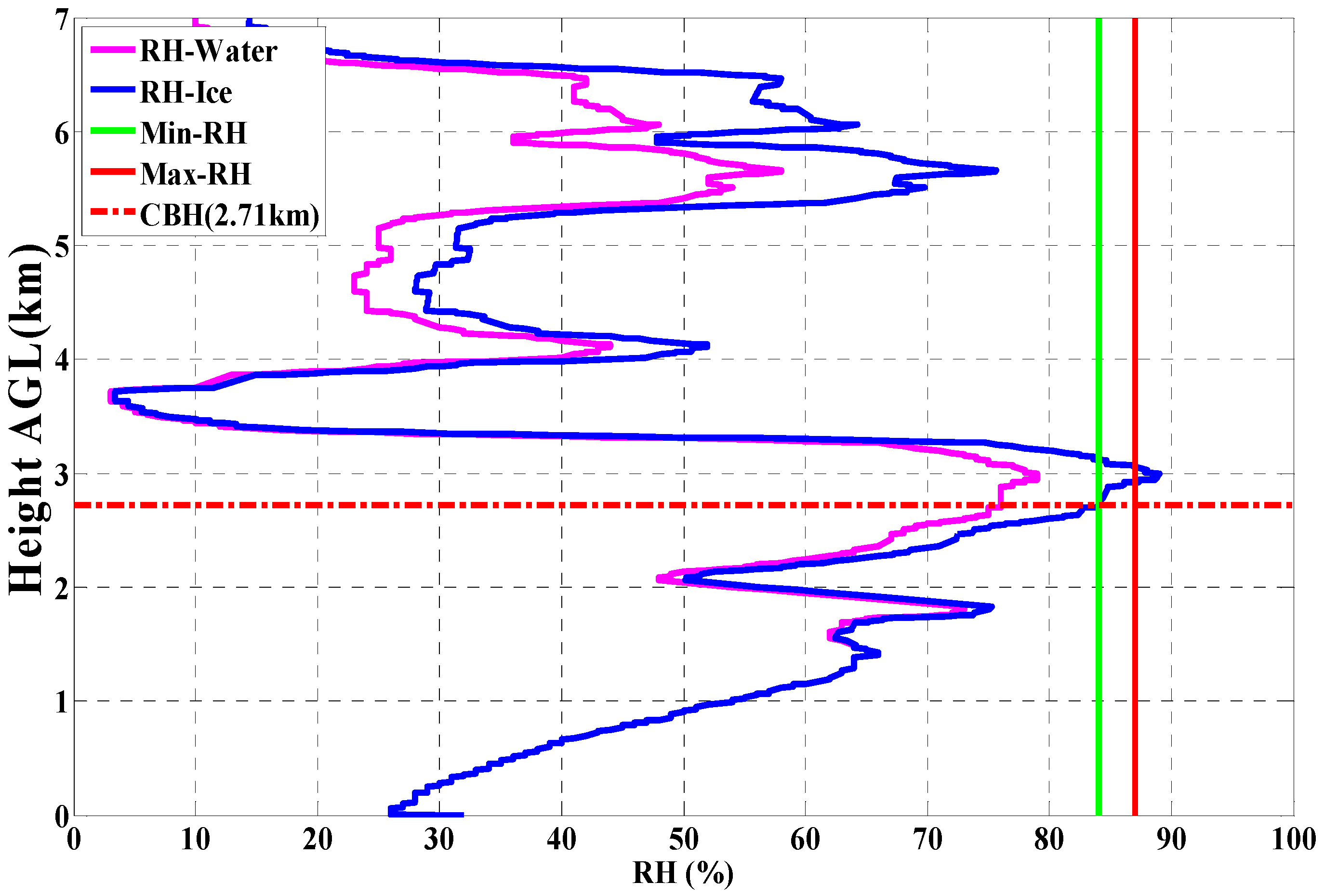
2.2.2. Relative Humidity (RH) Threshold Method Using Radiosonde

Radiosonde with high vertical resolution has been widely used to obtain atmospheric parameters including those of cloud vertical structure. Methods have been developed to determine locations of cloud layers and their boundaries from radiosonde measurement [24,25]. According to the radiosonde characteristics and Nagqu atmospheric conditions, the WR95 method [23] is used to obtain cloud vertical structure. The cloud base and top locations are identified using the following criteria: maximum RH ( R H m a x ) > 87%; minimum RH ( R H m i n ) > 84%; and the cloud base of the lowest layer of cloud is set at 500 m AGL. Moreover, the minimum thickness of low-middle cloud and high cloud are set to 30 m and 60 m, respectively, and the range of adjacent clouds should be larger than 300 m. It is noted that a transformation of RH with respect to ice at levels where the temperature is below 0 °C should be considered, that is,
R H n e w = R H × ( E w / E i )
where E w and E i are saturation vapor pressure of water and ice, respectively; and RH is the measured relative humidity of radiosonde. The calculation of E w and E i are based on GG46 and GG46i equations [26,27], respectively,
log 10 E w = 10.79574 ( 1 T 1 T ) 5.02800 log 10 ( T T 1 ) + 1.50475 × 10 4 [ 1 10 8.2969 ( 1 T / T 1 ) ] 0.42873 × 10 3 [ 1 10 4.76955 ( 1 T 1 / T ) ] + 0.78614
log 10 E i = 9.09685 ( 1 T 1 T ) 3.56654 log 10 ( T 1 T ) + 0.87682 ( 1 T T 1 ) + 0.78614
where T 1 = 273.15   K , T 1 = 273.15 + t , and t is centigrade temperature. Then, the cloud structure below 0 °C can be determined from Equations (1)–(3).

3. Results

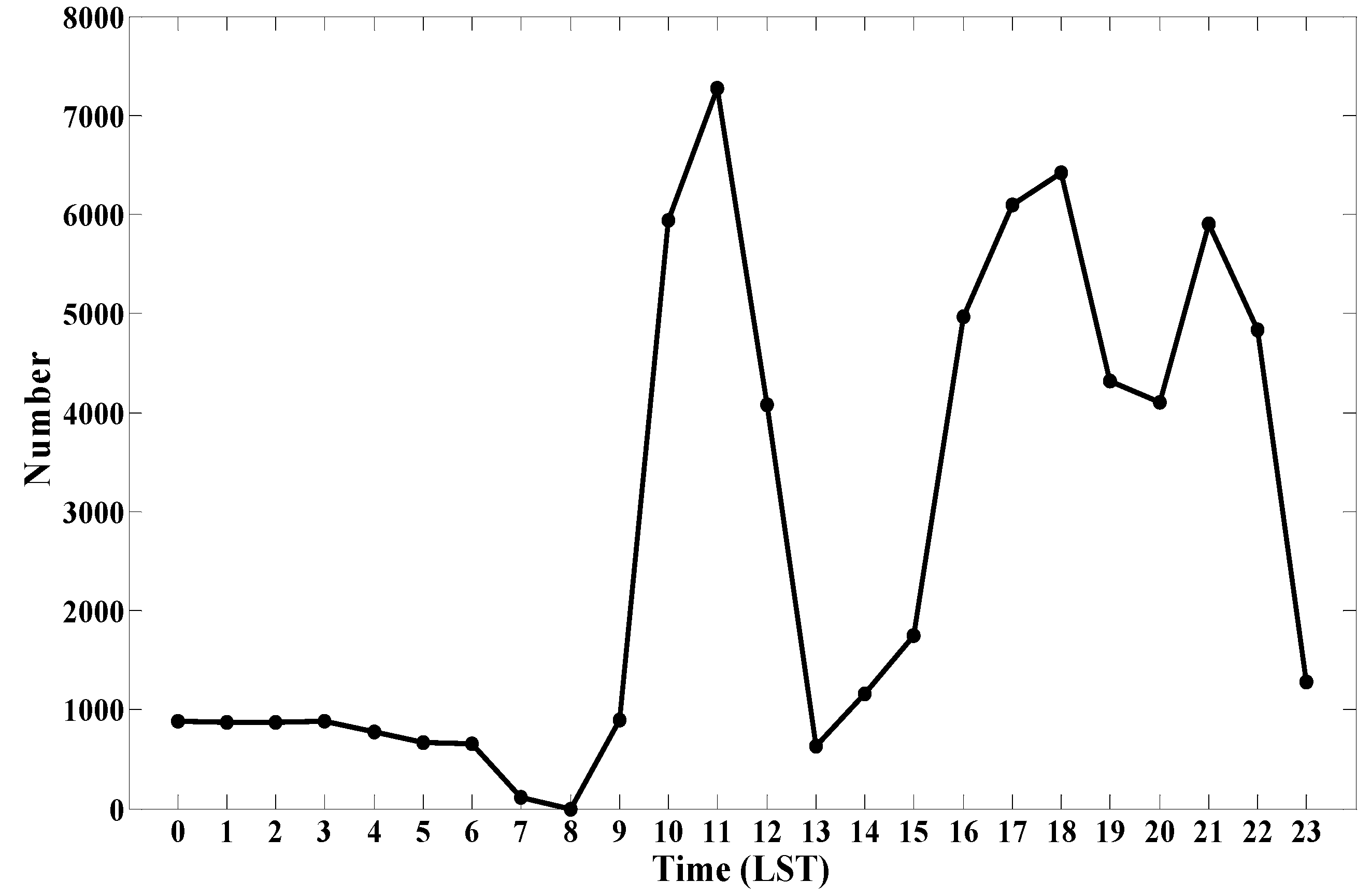
3.1. Cloud Characteristics Statistics of CL31

The data acquirability of CL31 is firstly analyzed to guarantee sufficient samples and the accuracy of follow-up work since there may exist data missing due to mistaken operative mode, although CL31 is in a 24-h continuous observation mode during the whole experiment period. The time resolution of CL31 is 16 s, thus one hour has 12,600 data size in the 56-day observations. Figure 5a is the data acquirability per hour, and the x-axis represents each 1-h interval over 24 h, for instance, the point at 1 represents the data acquirability between 00:00 and 01:00 Local Standard Time (LST, LST = UTC + 8 h). It can be seen that the data acquirability at 00:00–09:00 are all 100% with no data deficiency, and the others are all above 95%. Thus, the data missing level is endurable and reasonable, which has a negligible impact on the following statistical results.
It can be seen in Figure 5b that the cloud occurrence is about 81% during the experiment period, and the one-layer cloud has the highest occurrence frequency of 65% with multi-layer cloud frequency of 13%, so the cloud structure at Nagqu in summer is relatively simple. It is noted that sometimes CL31 “cloud status” is “4”, representing the atmospheric condition is full obscuration determined but no cloud base detected. In this case, the results represent “vertical visibility as calculated” and “highest signal detected”. During the experiment period, the occurrence of “4” almost happens in the rainy weather, its diurnal variation is obvious, the daytime occurrence is rare but has significant increase at night and before dawn, which corresponds to the special weather phenomenon of “sunny daytime, rainy nighttime” at Nagqu.
The cloud occurrence of CL31 is defined as the ratio of the cloudy profiles and the total profiles. The occurrence frequency of a specific layer cloud (e.g., one-layer cloud) at specific time interval is defined as ratio of the profiles having the specific layer cloud and the total profiles. It can be seen in Figure 6 that the averaged cloud occurrence is between 70% and 90% each day, which is consistent with the results from millimeter-wave radar and satellite data [13,28]. It can be also seen that the diurnal variation of cloud occurrence is obvious, that is, the cloud occurrence has a minimum value between 13:00 and 14:00 LST, and with the enhancement of the surface radiation, the atmospheric activities become more convective with cloud occurrence rapidly increasing. Moreover, the occurrence frequency of multilayer cloud is relative low and stable, on the other hand, the one-layer cloud occurrence frequency has an obvious variation with a maximum proportion.

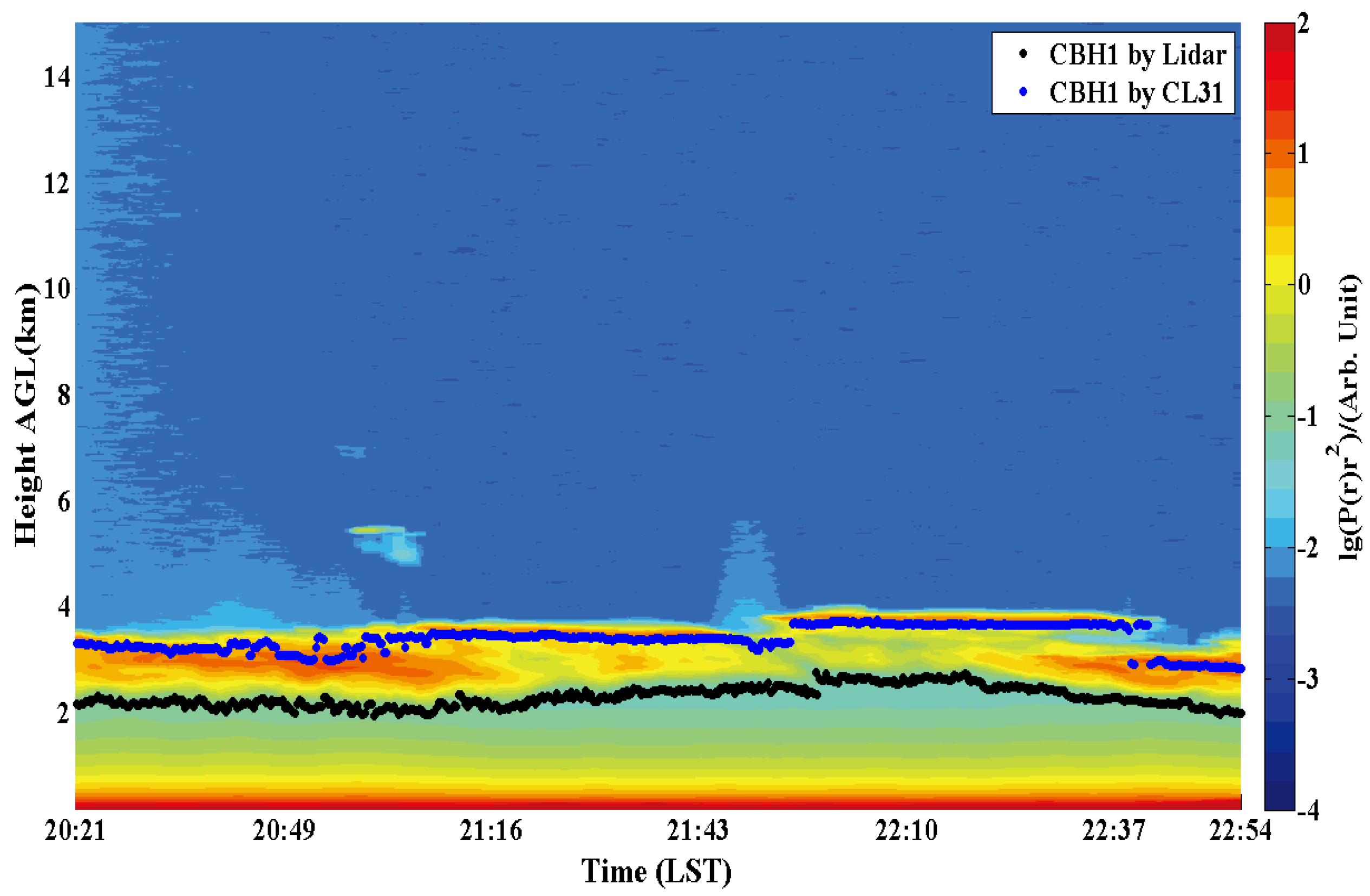
3.2. CBH Comparison between CL31 and WACAL

Comparisons between different types of instruments have shown typical features of instruments and provided many different phenomena of clouds [29,30,31]. Feister et al. [29] made a comparison of macroscopic cloud data from ground-based measurements using VIS/NIR and IR instruments and showed that CBH differences between the instruments in the lower height range are mainly due to the different principles of measurement including the geometries of measurements, the assumption on lapse rate used in the Nubiscope cloud algorithm, and the definition of CBH for the respective instrument. Liu et al. [30] used two ceilometers (CL31, CL51) and a whole-sky infrared cloud-measuring system and found that even if the same ceilometers with different types may introduce different observation results of CBH. Although the commercial ceilometer, like Vaisala CL31, has been extensively used in cloud study, the CBH retrieval algorithm still need to be investigated, especially to look into the data from different apparatus.
The comparison of first CBH (CBH1) between CL31 and WACAL has been analyzed in Figure 7. Noted that CL31 has the ability of 24-h continuous observation while the WACAL is only operated at about 09:00–12:00, 14:00–19:00, and 20:00–23:00 each day except for the passes of CALIPSO, the matching time should be based on the WACAL sampling time. Thus, the data every 4 min are chosen to compose the dataset with the number of 2610. In Figure 7, the red solid line and light blue dashed line represent the linear fit for all dataset and the data excluding | fdata-ydata | > 1 . 0 * SD , respectively, where fdata is the fitted value, ydata is the corresponding CL31 CBH, and SD represents the standard deviation of ydata. The black dashed line is the weighted least square fit for all dataset. The black and pink dots represent | fdata-ydata | within and without the standard deviation of ydata. The occurrence of the pink dots is mainly the result of different cloud layer comparison for these two devices. Non-strict time comparison may result in deviation in this process; moreover, when it occurs due to low thin cloud, CL31 sometimes has fault decision by mistake, resulting in different cloud layer comparison for these two devices. Basically, the CBH of CL31 and WACAL shows a good consistency with the correlation of 0.82 and standard deviation of 0.99 km. After excluding the singular value in pink dots, the correlation and standard deviation has been increased up to 0.92 and decreased to 0.64 km, respectively.
From the frequency distribution of the CBH differences shown in Figure 8a, it can be found that about 46% of the differences are within ±200 m, and about 80% of the differences are within ±1000 m. The deviation has an obvious left-skewed distribution; that is, the condition that WACAL CBH is smaller than CL31’s occurs much more often than the one that CL31 CBH is smaller than WACAL’s. Figure 8b shows the frequency distributions of CBH retrieved with WACAL and CL31 for the dataset, respectively. The histogram for all CBH together has the maximum for the bin cantered at 1000–2000 m, and shows a progressive decreasing frequency up to the maximum level of detection of the WACAL and CL31. It is clear that the cloud layers detected by WACAL are much more than CL31 in the range of 1000–2000 m.
In view of the above condition, a case study at 20:00–23:00, 12 August has been analyzed. Figure 9 shows the Time–Height–Intensity diagram of WACAL observation, where the black dots and blue dots represent the retrieved CBH by WACAL and CL31, respectively. It can be found that there exists obvious difference between these two results. This may be the result of the difference on the CBH definition and retrieval methods [26]. Specifically, the improved differential zero-crossing method of WACAL regards the place where the first derivative of the lidar backscatter power changes from negative to positive as the CBH, while the CL31 regards the strongest backscattered signal point as the CBH.
The cloud structure in this case is also retrieved using simultaneous radiosonde data and shown in Figure 10. The red and blue solid line represent the RH measured from the radiosonde and calculated from the saturation vapor pressure of ice using Equations (1)–(3), respectively. The CBH is 2.71 km using WR95 method mentioned in Section 2.2.2, and shows a good consistency with the WACAL result shown in Figure 9. It can be indicated that CL31 sometimes overestimates the CBH compared with WACAL and radiosonde, which to some extent explains the situation that WACAL CBH is smaller than CL31’s much more often than CL31 CBH is smaller than WACAL’s.

4. Discussion

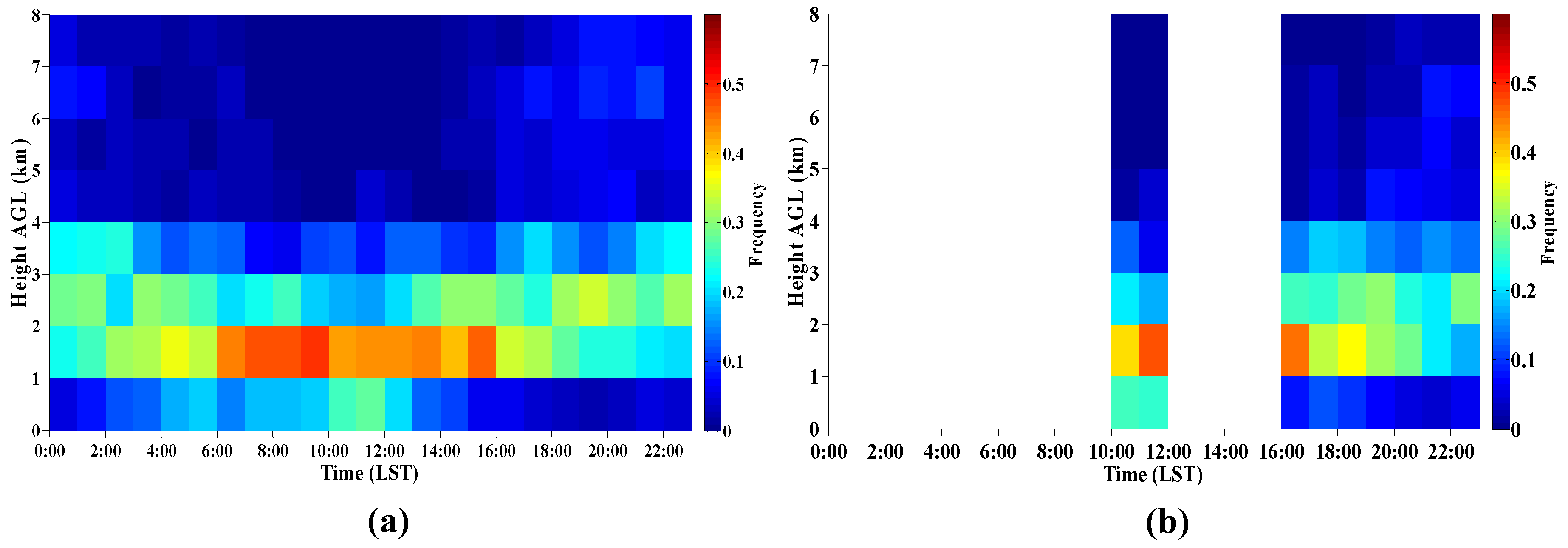
4.1. Cloud Characteristics Diurnal Variation Comparison between CL31 and WACAL

Since WACAL is not 24-h continuous observation like CL31, the data acquirability should be firstly analyzed to make the further work more reliable. Figure 11 shows the data acquirability per hour, and the x-axis represents each 1-h interval over 24 h, which is same as the Figure 5a. The time resolution of WACAL is 16 s, thus 1 h has 8325 data size in the 37-day observations from 8 July to 15 August. In this statistic, the hour with total observed number larger than 4000 is chosen to make comparison with CL31. As a result, 10 h, at 10:00, 11:00, 12:00, 16:00, 17:00, 18:00, 19:00, 20:00, 21:00 and 22:00, are selected as WACAL dataset for diurnal comparison. Moreover, the time period of 10:00–12:00, 16:00–19:00, and 20:00–22:00 can represent the cloud characteristics at forenoon, afternoon, and night period, respectively.
Figure 12a shows the averaged diurnal variation of CBH spatial distribution measured by CL31. The CBH distribution proportion at a specific time period and height range, for instance, from 00:00 LST to 01:00 LST at 1–2 km, is the ratio of the profiles where CBH occurs at 1–2 km to the total cloud layers at 00:00–01:00 LST. Note that the statistic is limited in the range from 0 m to 7.5 km due to the CL31 detection range limitation. It can be found that the CBH mainly occurred below 3 km with distinct diurnal variation. Specifically, the CBH is generally lower, below 2 km, at forenoon. With the increasing of surface radiation, the Plateau thermodynamic process becomes more active at afternoon so that the CBH is gradually lifted and high cloud begins to appear with a wider spatial scale. By evening, the vertical distribution of cloud reaches maximum value. Generally, the diurnal variation of CBH spatial distribution has a “U” shape; that is, high cloud mainly appears before dawn and at night, while, conversely, the low-middle cloud is the main cloud type during daytime. Figure 12b is the averaged diurnal variation of CBH spatial distribution measured by WACAL. The cloud analyzed range is selected as 0.5 km–7.5 km to make the data consistency with CL31’s. It can be seen that these two results have quite uniformity in distribution range, variation trend. A similar U shape distribution was also found using concurrent cloud radar measurement during the field experiment [13], and the distance between cloud radar, ceilometer and Lidar is about tens of meters, which can be regarded as the same area. Furthermore, the historical radiosonde observations from 136 ground-reference meteorological stations between 1987 and 2001 in China region have shown that the diurnal change of cloud occurrence has five types, single-peak in the morning, single-peak in the afternoon, double peaks with higher peak in the morning, double peaks with higher peak in the afternoon and double peaks with same value [32]. Unfortunately, there is no ground-reference meteorological station in the whole Tibetan Plateau. The reasons for the special U shape distribution cannot be explained well yet and should be further analyzed.
Figure 13a shows the averaged diurnal variation of CBH temporal distribution measured by CL31. The CBH frequency at a specific time period and height range, for instance, from 00:00 LST to 01:00 LST at 1–2 km, is the ratio of the profiles where CBH occurs at 1–2 km to the total profiles at 00:00–01:00 LST. It can be found that the diurnal variation of CBH frequency is similar to the CBH distribution proportion diurnal variation. In Figure 13a, the CBH frequency of low-middle cloud is obviously higher than the high cloud’s, and the high value area of low cloud occurs at 06:00–15:00. From 16:00 to the next morning, the CBH frequency of low cloud is relatively stable, ranging from 20% to 30%, while the CBH frequency of high cloud begins to increase gradually and reaches its maximum at night. Figure 13b is the averaged diurnal variation of CBH frequency measured by WACAL. Compared with CL31, both of them have a good consistency in distribution range and variation trend.

4.2. Cloud Characteristics Statistics of WACAL

Since the detection range limitation of CL31, the cloud below 7.5 km can only be measured, and the other cloud features such as the cloud top height and thickness are unattainable. However, the WACAL can fill these gaps because of its higher laser transmitting power and receiving ability, detecting wider range and retrieving accurately the cloud features in addition to the CBH. According to the results in Figure 11, the selected three time periods can represent different cloud development processes, so the cloud spatial-temporal distribution based on these three periods can be analyzed and compared using WACAL data. Figure 14 shows the averaged spatial distribution of one-, two-, three- and four-layer clouds measured by WACAL at forenoon, afternoon and night,. The CBT, CTH, Δ T (shown with green color in Figure 14), and N represent the averaged cloud base height, averaged cloud top height, averaged cloud thickness and the occurrence number of the specific cloud type, respectively. The value in bracket presents the corresponding occurrence frequency of the specific cloud type. It can be found that the cloud mainly occurs below 4 km with relative thinner cloud thickness in the forenoon, and the cloud structure of four-layer cloud is similar to the three-layer cloud’s, while the cloud has been lifted distinctly with all clouds getting thicker in the afternoon, the spatial scale has been extended to 6 km and the cloud structure of four-layer cloud is quite different from the three-layer cloud’s, whose top cloud thickness has developed from 0.19 km to 0.47 km. Till in the evening, the cloud continues to become higher and thicker with the spatial scale extending to 10 km, and the top cloud thickness of the four-layer cloud has developed to 1.07 km, which may be the result that the cooling effect of the lower cloud is relative drastic and results in the temperature stratification instability, causing more convective condition to contribute to the cloud development. Generally, the cloud development has obvious diurnal variation with a thicker, wider, and more abundant cloud structure process.

5. Conclusions

As a part of the TIPEX III, the Ocean University of China operated the CL31 and the WACAL from 7 July 2014 to 8 August 2014 to carry out the research on the microphysical characteristics and the vertical structure of cloud in Tibetan Plateau. This paper summarizes the CL31 and WACAL observations and comparisons of atmospheric cloud structure. The major findings are summarized below.
(1)
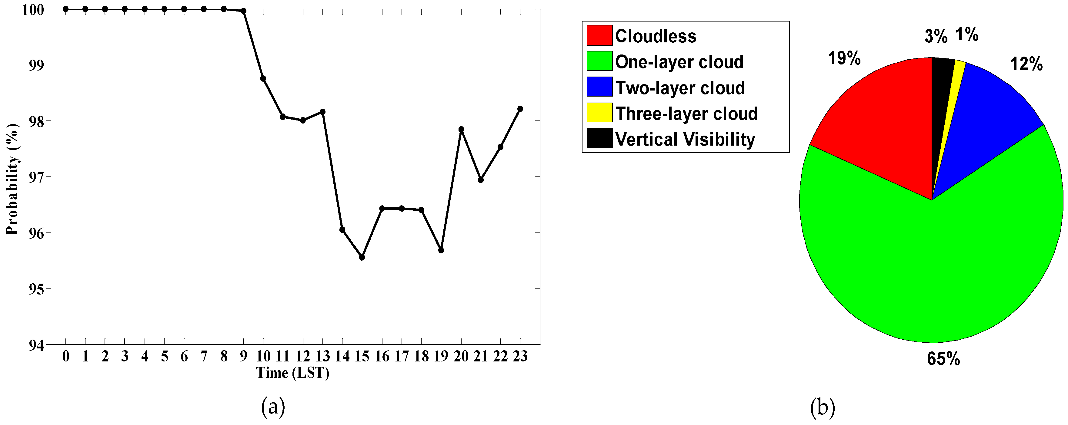
The cloud occurrence at Nagqu is about 81% during the CL31 experimental period with obviously diurnal variation. The cloud structure is relatively simple with a majority of single-layer cloud.
(2)
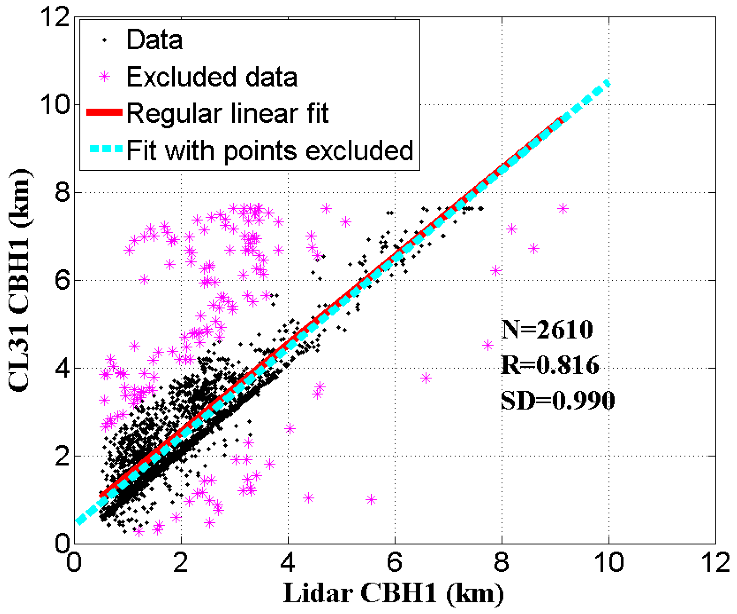
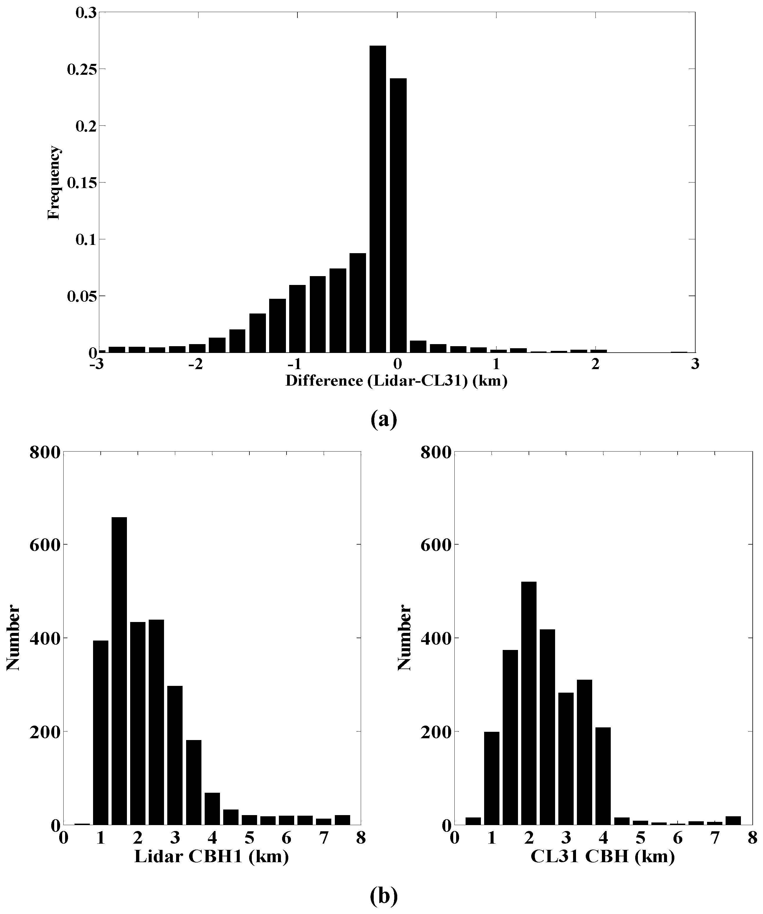
It can be found from the CBH comparison between CL31 and WACAL that the cases with obvious deviation may result from the different cloud layer detection from these two devices. The CL31 sometimes overestimates the CBH compared with WACAL’s on the premise that the same cloud layer is analyzed, which may be the result of the difference on the CBH definition and retrieval methods, and this phenomenon has also been validated by synchronous radiosonde result.
(3)
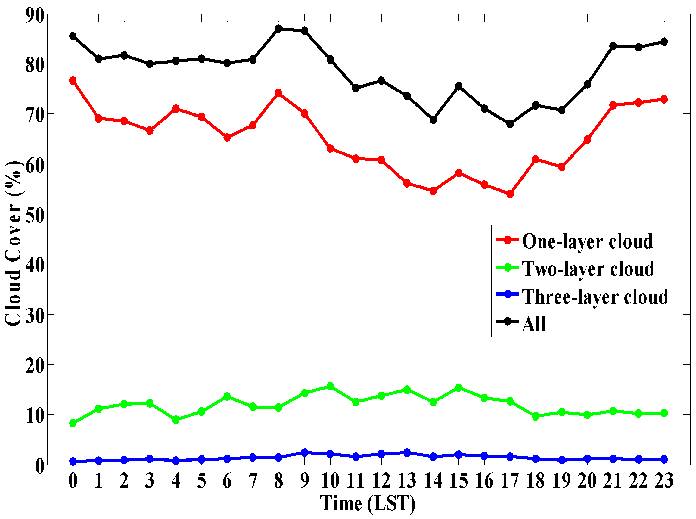
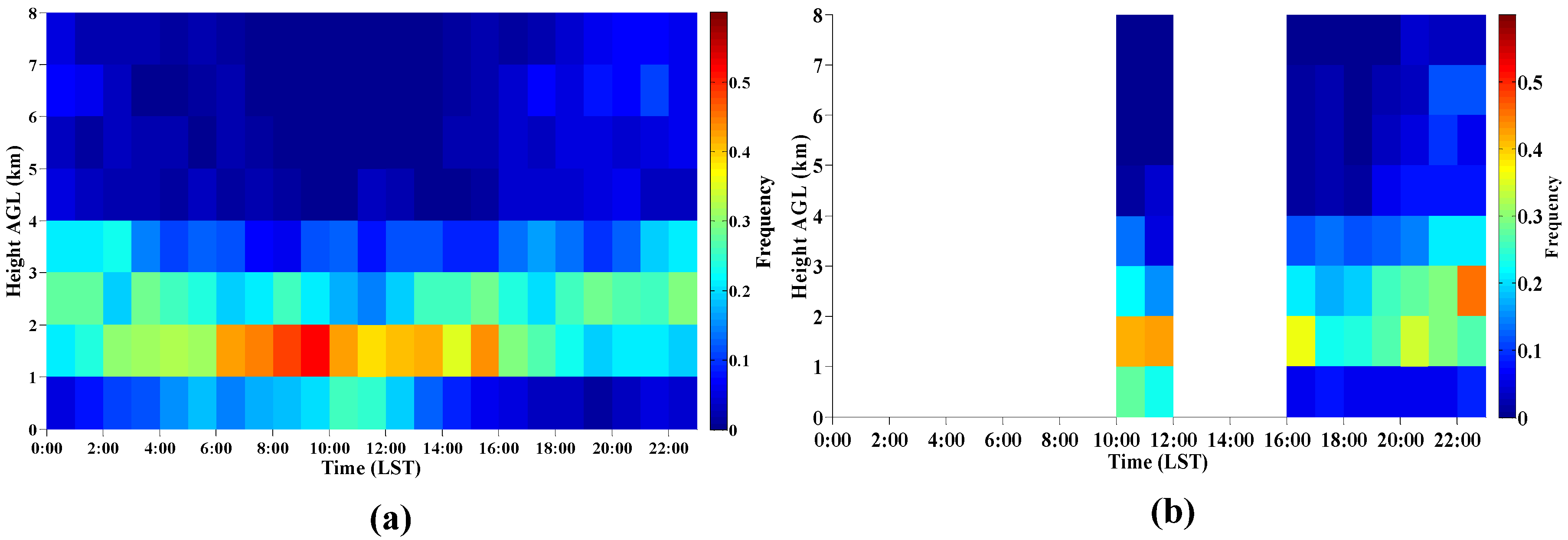
The diurnal variations of CBH distribution proportion and CBH frequency from CL31 observation have a similar variation trend with a distinct “U” shape, which analyze the cloud structure variation at spatial and temporal aspects, respectively. In addition, in the time snippet comparison between CL31 and WACAL, the results from these two devices have a good consistency in distribution range, variation trend, the corresponding high value area and so forth.
(4)
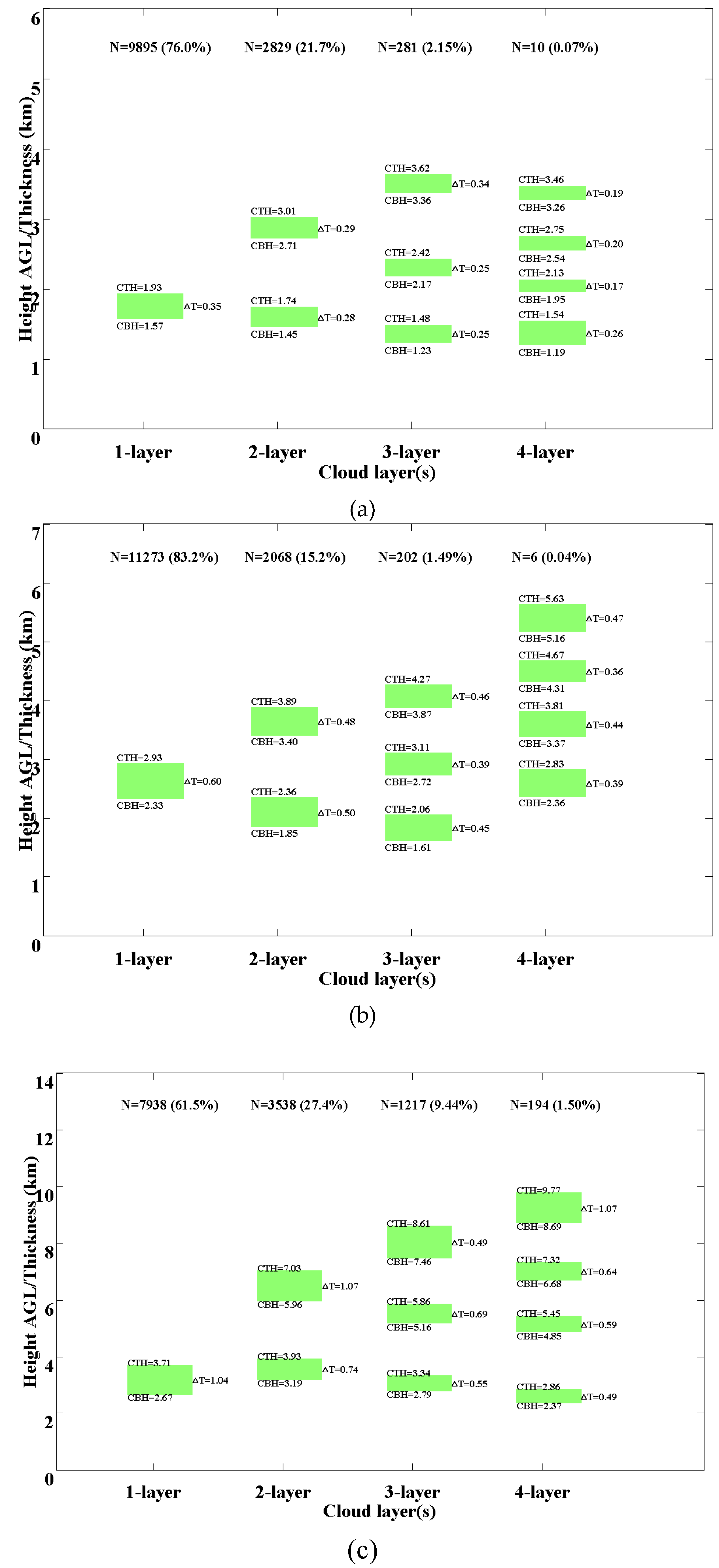
The WACAL compares the averaged spatial distribution of one-, two-, three-, and four-layer clouds from three different time periods, corresponding to different cloud development processes. The averaged cloud thickness and vertical distribution range at night is about 2.5–2.9 times and 2.4–3.3 times as much as the clouds in the forenoon, and the occurrence frequency of multi-layer cloud increases from 24% in the forenoon to 39% at night. Generally, the cloud development has a distinct diurnal variation with a thicker, wider, and more abundant cloud structure process.

Acknowledgments

This work was partly supported by the National Natural Science Foundation of China (NSFC) under grant 41375016, 41471309 and 91337103, by the China Special Fund for Meteorological Research in the Public Interest under grant GYHY201406001. We appreciate the contribution made by Meteorological Bureau of Tibet Autonomous Region, Nagqu Bureau of Meteorology. We also thank Guangyao Dai, Dongxiang Wang and Qian Zhang for their help with the observations and data processing.

Author Contributions

All authors made great contributions to the presented work. Xiaoquan Song and Xiaochun Zhai performed the algorithm and prepared the paper; Liping Liu and Songhua Wu designed the experiments and provided the technical discussions; and Xiaochun Zhai performed the experiments and analyzed the data.

Conflicts of Interest

The authors declare no conflict of interest.

References

  1. Myhre, G.; Samset, B.H.; Schulz, M.; Balkanski, Y.; Bauer, S.; Berntsen, T.K.; Bian, H.; Bellouin, N.; Chin, M.; Diehl, T.; et al. Radiative forcing of the direct aerosol effect from AeroCom Phase II simulations. Atmos. Chem. Phys. 2013, 13, 1853–1877. [Google Scholar] [CrossRef]
  2. Su, W.Y.; Loeb, N.G.; Schuster, G.L.; Chin, M.; Rose, F.G. Global all-sky shortwave direct radiative forcing of anthropogenic aerosols from combined satellite observations and GOCART simulations. J. Geophys. Res. Atmos. 2013, 118, 655–669. [Google Scholar] [CrossRef]
  3. Zelinka, M.D.; Dennis, L.H. Why is longwave cloud feedback positive? J. Geophys. Res. Atmos. 2010, 115, D16117. [Google Scholar] [CrossRef]
  4. Espinoza, H.R. Simple parameterizations of the radiative properties of cloud layers: A review. Atmos. Res. 1995, 35, 113–125. [Google Scholar] [CrossRef]
  5. Cess, R.D.; Potter, G.L.; Blanchet, J.P.; Boer, G.J.; Ghan, S.J.; Kiehl, J.T.; Treut, H.L.; Li, Z.X.; Liang, X.Z.; Mitchell, J.F.B.; et al. Interpretation of cloud-climate feedback as produced by 14 atmospheric general circulation models. Science 1989, 245, 513–516. [Google Scholar] [CrossRef] [PubMed]
  6. Stephens, G.L. Cloud feedbacks in the climate system: A critical review. J. Clim. 2005, 18, 237–273. [Google Scholar] [CrossRef]
  7. Jian, M.Q.; Luo, H.B. Impact of the diurnal variation of the surface heating in the Tibetan Plateau on the general circulation over the Asian monsoon region. J. Trop. Meteorol. 2002, 18, 269–275. [Google Scholar]
  8. Ye, D.Z.; Gao, Y.X. Qinghai-Xizang Plateau Meteorology, 1st ed.; Science Press: Beijing, China, 2002; pp. 1–278. [Google Scholar]
  9. Wang, H.; Luo, Y.L.; Zhang, R.R. Analyzing seasonal variation of clouds over the Asian monsoon regions and the Tibetan Plateau region using CloudSat/CALIPSO. Chin. J. Atmos. Sci. 2011, 35, 1117–1131. [Google Scholar]
  10. Zhao, Y.F.; Wang, D.H.; Yin, J.F. A study on cloud microphysical characteristics over the Tibetan Plateau using CloudSat data. J. Trop. Meteorol. 2014, 30, 239–248. [Google Scholar]
  11. Fu, Y.F.; Li, H.T.; Zi, Y. Case study of precipitation cloud structure viewed by TRMM satellite in a valley of Tibetan Plateau. Plateau Meteorol. 2007, 26, 98–106. [Google Scholar]
  12. Spinhirne, J.D. Micro pulse lidar. IEEE Trans. Geosci. Remote Sens. 1993, 31, 48–55. [Google Scholar] [CrossRef]
  13. Liu, L.P.; Zheng, J.F.; Ruan, Z.; Cui, Z.H.; Hu, Z.Q.; Wu, S.H.; Dai, G.Y.; Wu, Y.H. The preliminary analyses of the cloud properties over the Tibetan Plateau from the field experiments in clouds precipitation with the various radar. Acta Meteorol. Sin. 2015, 73, 635–647. [Google Scholar]
  14. He, Q.S.; Li, C.C.; Ma, J.Z.; Wang, H.Q.; Shi, G.M.; Liang, Z.R.; Luan, Q.; Geng, F.H.; Zhou, X.W. The properties and formation of cirrus clouds over the Tibetan Plateau based on summertime lidar measurements. J. Atmos. Sci. 2013, 70, 901–915. [Google Scholar] [CrossRef]
  15. Liu, C. Measurements of the Aerosol over Nagqu of Tibet and Suburb of Beijing by Micro Pulse Lidar (MPL). J. Photon. Study 2006, 35, 1435–1439. [Google Scholar]
  16. Yanai, M.; Li, C.; Song, Z. Seasonal heating of the Tibetan Plateau and its effects on the evolution of the Asian summer monsoon. J. Meteorol. Soc. Jpn. 1992, 70, 319–351. [Google Scholar]
  17. Vaisala Ceilometer CL31. Available online: https://sensorexperts.com/node/221729 (accessed on 21 April 2016).
  18. Wu, S.H.; Song, X.Q.; Liu, B.Y.; Dai, G.Y.; Liu, J.T.; Zhang, K.L.; Qin, S.G.; Hua, D.X.; Gao, F.; Liu, L.P. Mobile multi-wavelength polarization Raman lidar for water vapor, cloud and aerosol measurement. Opt. Express 2015, 23, 33870–33892. [Google Scholar] [CrossRef] [PubMed]
  19. GTS1 Digital Radiosonde. Available online: http://www.docin.com/p-1209358545.html (accessed on 21 April 2016).
  20. Winker, D.M.; Vaughan, M.A. Vertical distribution of clouds over Hampton, Virginia observed by lidar under the ECLIPS and FIRE ETO programs. Atmos. Res. 1994, 34, 117–133. [Google Scholar] [CrossRef]
  21. Pal, S.R.; Steinbrecht, W.; Carswell, A.I. Automated method for lidar determination of cloud-base height and vertical extent. Appl. Opt. 1992, 31, 1488–1494. [Google Scholar] [CrossRef] [PubMed]
  22. Wang, X.P.; Song, X.Q.; Yan, B.D.; Chen, C.; Liu, B.Y.; Wu, S.H. Research on the observation of cloud-base height for the city of Zhuhai of China with lidar. J. Optoelectron. Laser 2013, 11, 2192–2197. [Google Scholar]
  23. Wang, J.; Rossow, W.B. Determination of cloud vertical structure from upper-air observations. J. Appl. Meteorol. 1995, 34, 2243–2258. [Google Scholar] [CrossRef]
  24. Zhang, J.Q.; Chen, H.B.; Li, Z.Q.; Fan, X.H.; Peng, L.; Yu, Y.; Cribb, M. Analysis of cloud layer structure in Shouxian, China using RS92 radiosonde aided by 95 GHz cloud radar. J. Geophys. Res. Atmos. 2010, 115, D00K30. [Google Scholar] [CrossRef]
  25. Wang, J.; Rossow, W.B.; Uttal, T.; Rozendaal, M. Variability of cloud vertical structure during ASTEX observed from a combination of rawinsonde, radar, ceilometer, and satellite. Mon. Weather Rev. 1999, 127, 2482–2502. [Google Scholar] [CrossRef]
  26. Goff, J.A.; Gratch, S. Low-pressure properties of water from −160 to 212 F. Trans. Am. Soc. Heat. Vent. Eng. 1946, 51, 125–164. [Google Scholar]
  27. Alduchov, O.A.; Eskridge, R.E. Improved Magnus form approximation of saturation vapor pressure. J. Appl. Meteorol. 1996, 35, 601–609. [Google Scholar] [CrossRef]
  28. Eberhard, W.L. Cloud signals from lidar and rotating beam ceilometer compared with pilot ceiling. J. Atmos. Ocean. Technol. 1986, 3, 499–512. [Google Scholar] [CrossRef]
  29. Feister, U.; Möller, H.; Sattler, T.; Shields, J.; Görsdorf, U.; Güldner, J. Comparison of macroscopic cloud data from ground-based measurements using VIS/NIR and IR instruments at Lindenberg, Germany. Atmos. Res. 2010, 96, 395–407. [Google Scholar] [CrossRef]
  30. Liu, L.; Sun, X.J.; Liu, X.C.; Gao, T.C.; Zhao, S.J. Comparison of Cloud Base Height Derived from a Ground-Based Infrared Cloud Measurement and Two Ceilometers. Adv. Meteorol. 2015, 2015, 853861. [Google Scholar] [CrossRef]
  31. Van Tricht, K.; Gorodetskaya, I.V.; Lhermitte, S.; Turner, D.D.; Schween, J.H.; Van Lipzig, N.P.M. An improved algorithm for polar cloud-base detection by ceilometer over the ice sheets. Atmos. Meas. Tech. 2014, 7, 1153–1167. [Google Scholar] [CrossRef] [Green Version]
  32. Wang, B.M.; Liu, X.N. The cloud diurnal variation in China. In Cloud Distribution of China, 1st ed.; Chen, H., Ed.; China Meteorological Press: Beijing, China, 2009; Volume 8, pp. 82–106. [Google Scholar]
Figure 1. Location of the experimental observation site and the topography of the Tibetan Plateau (DEM: Digital Elevation Model).
Atmosphere 08 00009 g001
Figure 2. Pictures of: (a) CL31; and (b) WACAL.
Atmosphere 08 00009 g002
Figure 3. Flow chart of cloud properties retrieval based on improved zero-crossing method.
Atmosphere 08 00009 g003
Figure 4. Case study using improved differential zero-crossing method [22].
Atmosphere 08 00009 g004
Figure 5. CL31 (a) Data acquirability; and (b) the probability distribution of cloudless (red), one-layer cloud (green), two-layer cloud (blue), three-layer cloud (yellow) and vertical visibility (black) during the experiment period.
Atmosphere 08 00009 g005
Figure 6. Averaged diurnal variation of the cloud occurrence (black), one-layer cloud (red), two-layer cloud (green), and three-layer cloud (blue) of CL31 during the measurement period.
Atmosphere 08 00009 g006
Figure 7. Scatter diagram of the CBH1 measured by WACAL and CL31.
Atmosphere 08 00009 g007
Figure 8. (a) CBH1 difference between WACAL; and (b) distribution of the CBH1 of WACAL (left) and CL31 (right) during the measurement period.
Atmosphere 08 00009 g008
Figure 9. Atmospheric backscattered signal of WACAL at 20:21–22:54, 12 August 2014 and CBH1 measured by WACAL (black) and CL31 (blue).
Atmosphere 08 00009 g009
Figure 10. Radiosonde relative humidity (RH) profile and results of observed cloud structure.
Atmosphere 08 00009 g010
Figure 11. WACAL data acquirability during measurement period.
Atmosphere 08 00009 g011
Figure 12. Averaged diurnal variation of CBH spatial distribution measured by: (a) CL31; and (b) WACAL during measurement period.
Atmosphere 08 00009 g012
Figure 13. Averaged diurnal variation of CBH temporal distribution measured by: (a) CL31; and (b) WACAL during measurement period.
Atmosphere 08 00009 g013
Figure 14. Averaged spatial distribution of one-, two-, three-, and four-layer clouds measured by WACAL at: (a) forenoon (10:00–12:00); (b) afternoon (16:00–19:00); and (c) night (20:00–22:00).
Atmosphere 08 00009 g014
Table 1. Component parameters of the WACAL system and CL31.
SpecificationCL31WACAL
Laser typeInGaAs diodeNd:YAG
Wavelength (nm)910354.7/532/1064
Pulse energy (mJ)0.0012410/120/700
Repetition rate (kHz)100.03
Telescope/aperture (mm)Single Lens/96Light Bridge/304.8
Detection range (km)0–7.60.05–25
Range resolution (m)53.75
Temporal resolution (s)2–120 programmable1–120 programmable
Table 2. Component parameters of the GTS1 radiosonde.
Meteorological SensorSpecificationTechnical Parameter
TemperatureRange−90–50 °C
Accuracy (standard deviation)0.2 °C (−80–50 °C)
0.3 °C (−90–−80 °C)
Resolution0.1 °C
HumidityRange0% RH~100% RH
Accuracy (standard deviation)5% RH ( T 25   ° C )
10% RH ( T 25   ° C )
Resolution1% RH
PressureRange1060 hPa~5 hPa
Accuracy (standard deviation)2 hPa (1050 hPa~500 hPa)
1 hPa (500 hPa~5 hPa)
Resolution0.1 hPa
Table 3. Tuning standard of threshold value in different altitude and time range.
AltitudeTime RangeThreshold Value a
0.5–5 kmdaytime2–4
nighttime
5–10 kmdaytime1–1.5
nighttime20–30
>10 kmdaytime1–1.5
nighttime10–20

