Abstract
Surface clutter interference will be one of the important problems for the future of geostationary spaceborne weather radar (GSWR). The aim of this work is to provide some numerical analyses on surface clutter interference and part of the performance evaluation for the future implementation of GSWR. The received powers of rain echoes, land and sea surfaces from a radar scattering volume are calculated numerically based on the derived radar equations, assuming a uniform rain layer and appropriate land and sea surface scattering models. An antenna pattern function based on a Bessel curve and Taylor weighting is considered to approximate the realistic spherical antenna of a GSWR. The power ratio of the rain echo signal to clutter (SCR) is then used to evaluate the extension of surface clutter interference. The study demonstrates that the entire region of surface clutter interference in GSWR will be wider than those in tropical rainfall measuring mission precipitation radar (TRMM PR). Most strong surface clutter comes from the antenna mainlobe, and the decrease of clutter contamination through reducing the level of the antenna sidelobe and range sidelobe are not obvious. In addition, the clutter interference is easily affected by rain attenuation in the Ka-band. When rain intensity is greater than 10 mm/h, most of rain echoes at off-nadir scanning angles will not be interfered by surface clutter.
1. Introduction
Hurricanes or typhoons have always been among the most devastating natural phenomena on Earth, capable of spreading destruction and loss of life across wide areas. In the past ten years, a geostationary spaceborne weather radar instrument concept (GSWR) known as “NEXRAD in space” has been proposed to improve the monitoring and prediction of hurricanes or typhoons [1,2,3]. It is agreed that the GSWR would provide a breakthrough with regard to the observation of hurricanes or typhoons because the GSWR would be the first instrument capable of accomplishing hurricane observation at time scales less than hours [4]. However, one of the many problems in implementing GSWR is clutter from the surface, particularly at the large scan angles for good coverage from geostationary orbit [5]. The surface clutter is also a problem for tropical rainfall measuring mission precipitation radar (TRMM PR) [6,7,8,9,10] and global precipitation mission dual-frequency precipitation radar (GPM DPR) [11,12,13].
Surface clutter echoes can be received by spaceborne precipitation radar from the antenna mainlobe (ML), sidelobe (SL), and range sidelobe (RSL). It is necessary to evaluate how seriously surface clutter will contaminate the rain echoes before their actual implementation, which can help the radar designers to make a decision on what level of antenna sidelobe or range sidelobe they should meet. Before the implementation of TRMM PR and GPM DPR, much work has been done on the evaluation and reduction of surface clutter [6,7,8]. Hanado and Ihara [7] inferred the power equation of surface clutter from the geometry of TRMM PR and the basic radar meteorological equation. Their results showed that the masked regions of surface clutter extended to an altitude of 1.2 km for an incidence angle of 17°. Durden et al. [9] specifically analyzed the surface clutter power from the antenna sidelobe, including other effects from the transmitted pulse, Doppler shifting, finite receiver bandwidth, and the Earth’s curved surface. Based on the methods in [7], Tagawa et al. [12] also calculated the surface clutter interference with precipitation measurement using 35.5 GHz radar for the GPM DPR. Results indicated that the interference of surface clutter from the antenna main lobe is serious and cannot be negligible either in light or heavy rain. In addition, Yin et al. [14,15,16] also computed the power of sea clutter interference for the dual-frequency precipitation radar (DPR) of the Chinese FengYun-3 (FY3) precipitation measurement satellite. Based on the analysis of surface clutter, the requirements for antenna beam width and sidelobe level are proposed. Even in the system design of future spaceborne cloud radar, the surface clutter is one of the many problems which should be dealt with carefully in the design of the antenna and pulse compression [17].
In order to reduce the effects of clutter inference and improve the data quality of radar products, much work has also been proposed for the radar design, the scan strategy, or the post-processing method on level-2 products. Tagawa [11] proposed a new method to suppress the antenna sidelobe clutter interference which tilts the antenna beam scan plane from nadir. T Kubota [18] presents a statistical method to reduce sidelobe clutter for observed data of Ku-band radar in GPM PR. Durden and Tanelli [5] described a Doppler filter approach to clutter suppression for GWDR. However, the premise of these works is that they have firstly known how seriously the surface clutter will contaminate the rain echoes.
GSWR is a future precipitation radar concept which will be firstly designed for geostationary orbit. Many of problems should be understood and resolved completely before progressing into final design and implementation. How seriously surface clutter will contaminate the rain echoes is one of the many problems which should be evaluated and analyzed before implementation, as well as which level of antenna mainlobe, sidelobe, and range sidelobe should be needed in the design of the antenna and pulse compression technique to alleviate the surface clutter contamination. In addition, due to the geostationary orbit, some clutter suppression technique, such as a frequency-domain filter, will be applied in the surface clutter reduction for GSWR.
In this paper, we calculated the power of sea and land surface clutter based on the geometry of the geostationary orbit and the proposed parameters of the GSWR, and finally analyzed the effects of the antenna main lobe, sidelobe, and range sidelobe to clutter interference. This aim is to obtain the effects of clutter interference to rain echoes and the level of antenna sidelobe and range sidelobe in future GWDR. The results of receiving power distribution and the ratio of rain echo signals to clutter (SCR) from sea and land surface clutter are used for these evaluations, which show that the whole region of clutter interference is much wider than those in TRMM PR, but it can be decreased sharply due to attenuation in heavy rain.
2. Methods of Surface Clutter Calculation
2.1. Surface Clutter Calculation
The GSWR was designed to work in geostationary orbit at an altitude of 36,000 km and operate at a frequency of 35 GHz. A deployable, 35 m spherical antenna reflector together with two antenna feeds were used to perform spiral scans from nadir to 4° to cover a 5300-km circular disk on the Earth’s surface [3,4]. The geometry of the spiral scan pattern of the GSWR is shown in Figure 1a, with a beamwidth of 0.019°, the corresponding horizontal resolution of the GSWR ranges from 12 km at nadir to 14 km at 4° scan. As shown in Figure 1b,c, surface clutter echoes from the antenna main lobe, sidelobe, and range sidelobe are received simultaneously by the radar receiver with rain echoes, which will prevent exact measurement of the rain echoes.
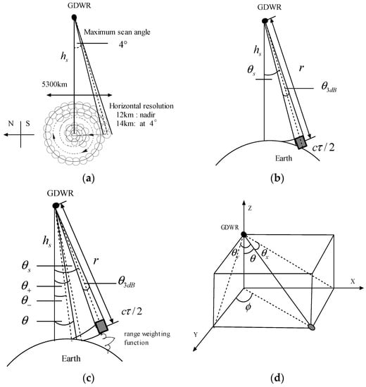
Figure 1.
Geometry of the surface clutter interference in a geostationary spaceborne weather radar. The altitude of the geostationary orbit is 36,000 km and the scan angle is from nadir to 4°. (a) Spiral scan mode; GSWR performs the spiral scan from nadir to 4° and its maximum horizontal resolution at 4° is nearly 14 km; (b) diagram of antenna mainlobe clutter; the grey square shows the radar range bin in which the antenna main beam has touched the earth surface; (c) diagram of the antenna sidelobe clutter and range sidelobe; the grey square shows the radar range bin in which antenna SL has touched the Earth’s surface, but the antenna main beam did not. It also shows the radar range bin that the range sidelobe will affect; (d) The geometry relation of incident angle , azimuthal angle with beam direction angles .
Although GSWR in the geostationary platform has a different spiral scan pattern and a different geometry relationship with the Earth, the main methods of surface clutter calculation are similar with those used for TRMM PR [7,8,9,10] and GPM DPR [11,12,13], except that the surface clutter from range sidelobe will be particularly considered. We rewrite the radar equation of the surface clutter calculation here. The received power of surface clutter in the same range with rain echoes through these three different methods above could be calculated by one integration equation along the surface area [7,19]:
where is the transmitting power, is the radar wavelength, is the incident angle, is the azimuthal angle, is the range from the radar. The polar coordinate system (, , ) denotes the distance from radar, the polar angle and the azimuthal angle. is the antenna pattern, is the range weighting function, is the normalized radar cross-section (NRCS), and is the integration unit of area. is the rain attenuation:
As shown in Figure 1c, the surface clutter in those range bins whose main beam does not touch the surface are mostly caused by the antenna sidelobe and range sidelobe. In these conditions the integration unit of area can be converted into the integration of incident angle and azimuthal angle [7,8,9]:
Thus, the final radar equation for calculating surface clutter from the antenna sidelobe and range sidelobe can be written as the integration over and [7,8,9,11,12,13,14]:
where is the -integrated squared pattern:
For simplification, we assumed that the surface clutter backscatter is independent of the azimuthal angle . Thus, if we ignore the effects of to , we can calculate the integration (Equation (4)) over firstly. The integrated interval between and is determined by the altitude of the satellite platform, the transmitting pulse width, and range resolution [7,8,9]. Considering the curvature of the Earth in calculating the integrated interval, the border of these two angles can be derived through the cosine theorem:
where is the satellite altitude, and is the Earth’s radius. When the main lobe of the antenna intersects the surface over an area , then the surface clutter from the main lobe can be written as:
With the changes of the incident angles, can be calculated by:
where is the corresponding grazing angle to the scan angle . If not ignoring the curvature of the Earth, they have the relationship:
The power of rain echoes can also be obtained through the integration of the radar equation over the backscattering volume, which is determined by the antenna beamwidth and range resolution. Here we directly use the integrated radar equation [15]:
where is the antenna gain, is the range-weighting function, is the radar reflectivity, and is the distance from the center of range bin. In the radar equation above, it was supposed that rain distribution in the volume is uniform and the antenna beamwidth is Gaussian. Since the power of the surface clutter from the range sidelobe will be calculated, the integration over the range direction could not be ignored.
2.2. Antenna Pattern Function
As shown in Equation (1), an antenna pattern function is needed to calculate the power of the surface clutter. A technique with a deployable spherical reflector for GSWR was proposed in [2,3] and its simulation result the antenna pattern function was given, whose sidelobe is expected to be less than −30 dB. In this paper, we designed the antenna pattern function based on a Bessel curve and Taylor window to approximate those shown in [2,3]. The pattern function based on Bessel curve in the far field can be written as [20,21]:
where is the diameter of the antenna. is the first-order Bessel function. , are separatly the beam angles in coordinate plane of X-Z and Y-Z, which is shown in Figure 1d. The transfering relation between these two planes can be expressed as follows
, are separately the antenna beamwidth along the direction in coordinate plane of X-Z and Y-Z, which are designed for the same beamwidth of 0.02°. The sidelobe of the antenna pattern function based on Equation (11) above is only −13 dB, so this pattern function is then weighted through Taylor window to decrease the sidelobe. This final normalized antenna pattern in one- and two-dimensions is shown in Figure 2. The sidelobe of the antenna is designed to −30 dB which is close to the requirements of the GSWR concept design.
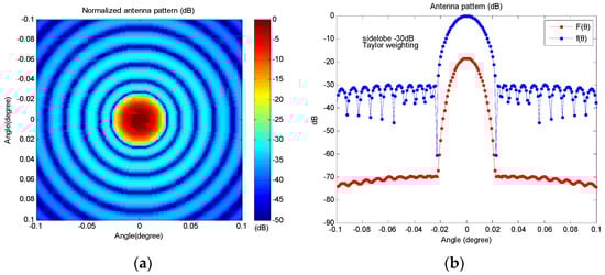
Figure 2.
Antenna pattern of a parabolic reflector antenna with −30 dB Taylor weighting and its integrated squared antenna pattern . (a) Two dimension antenna pattern along beam direction angles calculated from Equation (11) and Taylor window; (b) Antenna pattern and its integrated squared antenna pattern at nadir.
2.3. Range Weighting Function
GSWR will use a linear frequency modulated signal (LFM) to transmit and enhance its detection ability. The technique of sidelobe suppression in pulse compression is important to decrease the effects of surface clutter. To calculate the power of surface clutter from the range sidelobe, a range weighting function must be obtained first. The range ambiguity function of LFM can be written as [15]:
where B is the signal bandwidth, and is the pulse width of the transmitter. Its normalized range weighting function can be expressed as:
where is the distance from the center of the range resolution . However, the level of the range sidelobe based on a match filter on the LFM signal can only be about −13 dB. Other methods, like weighting on the LFM signal before transmitting or windowing on a match filter after receiving, are adopted to decrease the level of the range sidelobe. For example, we can obtain the range sidelobe at less than −40 dB through using a Hanning window on the received LFM signal. If a Taylor function is used on the transmitting LFM signal, a range sidelobe less than −60 dB can be obtained [14,15]. In order to evaluate the effect of the range sidelobe level to surface clutter, both of these two methods are used to produce the range weighting function of the range sidelobe from −40 dB to −55 dB in this paper.
2.4. Surface Clutter Scatter Model
The model of surface clutter scatters often need to be classified into types: land surface and sea surface. Due to the complex vegetation covering and various terrains on the land surface, it was difficult to build a uniform model to determine the backscattering of the land surface. Although the sea surface backscattering was affected by a large number of factors, such as surface roughness, grazing angle, polarization, etc., the sea surface backscattering within an incident angle less than ±20° can be expressed as a quasi-specular scattering model [7,8,9]. In this paper, we adopted the normalized radar cross-section (NRCS) of the land surface and sea surface measured by Grant and Yaplee [22] from the Ka-band radar, which was also used to calculate the surface clutter interference for FY3 DPR [14,15]. In their experiments, land surface with different terrains, and sea surface with different wind speeds, was observed with the incident angles from 0° to 80°. Due to the angle interval of 5° in their experiments, we now use a method of three-sample interpolation to obtain the NRCS at a high interval of 0.02°. The results are shown in Figure 3. In addition, we also use the results of NRCS investigated by Satake and Hanado [23], Tanelli et al. [24]. Satake has obtained the characteristics of NRCS from Ku-band TRMM PR for some terrains at designated places, such as the Amazon rainforest, Libyan Desert, and the East China Sea. Tanelli investigated the characteristics of NRCS from simultaneous Ku-band and Ka-band measurements by the dual-frequency Airborne Precipitation Radar (APR-2), which can provide some results of NRCS about the sea surface. In order to differentiate these three research results of NRCS, the signs of researchers’ abbreviated names are used in Figure 3. Signs of G.Y, S.H, T.D separately show the NRCS data from Grant and Yaplee [22], Satake and Hanado [23], and Tanelli and Durden [24]. Among these three types of NRCS, the advantage of NRCS from Grant and Yaplee was that the data is measured by a Ka-band radar with incident angles greater than 30°, but the radar beamwidth was rather larger. On the contrary, the NRCS from [23] was measured by TRMM PR with a narrower beamwidth, but the incident angle was limited within angles of 20° which needed interpolation. However, as shown in Figure 3a, the trend of three NRCS curves of the sea surface with larger wind speeds from [22,23,24] are similar.
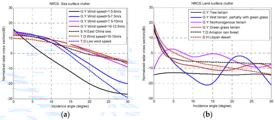
Figure 3.
Normalized radar cross-section of sea and land surface clutter under different incidence angles; (a) sea surface clutter; G.Y, S.H, T.D separately show the NRCS data from Grant and Yaplee [22], Satake and Hanado [23], and Tanelli and Durden [24]; (b) land surface clutter.
3. Results and Discussion
The numerical experiments are developed and discussed in the following ways. Firstly, the powers of surface clutter from land and sea surfaces are calculated and analyzed by assuming no rain attenuation. The antenna sidelobe level of −30 dB and range sidelobe level of −55 dB are used based on the radar system parameter proposed in [2,3]. Then, assuming that the rain layer is uniform, the power of rain echo and its signal-to-clutter ratio (SCR), are calculated. The SCR is defined as , where is the power of rain echo in the same range bin with the surface clutter. and are separately calculated by Equations (1) and (10). Usually, those regions with SCR less than 0 dB mean clutter interference are more serious. The less the SCR is below 0 dB, the more serious is the clutter interference. Thus, the SCR values below 0 dB are used to evaluate how seriously the surface clutter would affect the rain measurement of GSWR. Finally, after changing the antenna beamwidth, sidelobe, and range sidelobe, the powers of surface clutter and rain echoes and their corresponding SCR are recalculated, which will show different effects of clutter interference. This can provide one of the requirements for the design of the antenna and pulse compression technique. However, it is worth saying that the range sidelobe level of −55 dB is chosen so that the range sidelobe effect is minimized, and the experiments before Section 3.4 will be focused on the clutter effects from the main and sidelobe of the antenna.
In these experiments, the powers of surface clutter and rain echoes are calculated based on Equations (1) and (10). The parameters of GSWR system are shown in Table 1. The altitude of geostationary orbit is 36,000 km and the radar beamwidth at azimuth and the pitch direction are supposed to be symmetric. The minimum detected power of the radar receiver is computed from the minimum reflectivity after the pulse average shown in Table 1. In the model of precipitation, a uniform stratiform rain layer with height of 6 km is assumed. For simplification, the rain attenuation is only considered based on the k-Z relation shown in Table 1.

Table 1.
GSWR radar parameters.
3.1. Power of Surface Clutter
The powers of different sea surface and land surface clutter are separately shown in Figure 4 and Figure 5. In these figures, the x-axis indicates the spiral-scan angles from nadir to the maximum scan angle of 4°, while the y-axis is the altitude which is decided by the radar range and the incident angles of the radar beam. The red and blue lines in the figures show the region borders of the antenna mainlobe clutter, sidelobe clutter, and clutter free area, which can directly indicate what factors they are caused by. The methods of border calculation are the ones used by Tetsuya Tagawa [11] and the width of the mainlobe is set to two times of beamwidth, which can be seen in Figure 2b. In addition, only those power values greater than the radar minimum sensitivity are presented in color because those less than the radar minimum sensitivity are thought not to be detected by the radar receiver.
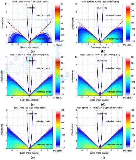
Figure 4.
Power distribution (dBm) of sea clutter at different spiral scan angle, without rain attenuation. The figures only show those power values of sea surface clutter greater than the radar receiver’s sensitivity (−122 dBm after pulse-average). (a) Wind-speed: 1–5 m/s; (b) Wind-speed: 5–7.5 m/s; (c) Wind-speed: 7.5–10 m/s; (d) Wind-speed: 10–12.5 m/s; (e) East China sea, NRCS data from TRMM PR; and (f) wind-speed: 10–15 m/s, NRCS data from APR-2. The surface clutter powers are proportional to the normalized radar cross-section of sea surface in different scan angles.
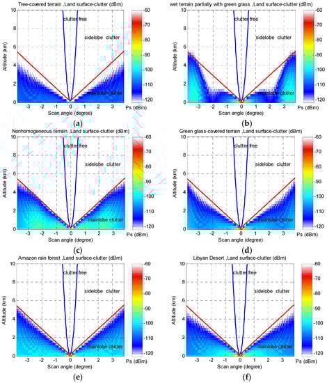
Figure 5.
Power distribution (dBm) of land surface clutter at different spiral scan angle, without rain attenuation. (a) The terrain of Amazon rain forest; (b) terrain covered with wet terrain, partially with green grass; (c) a nonhomogeneous terrain, such as sand, marsh, and bushes; (d) a terrain covered with tall green weeds; (e) the terrain of the Amazon rainforest; and (f) the terrain of Libyan desert.
Figure 4 shows the power distribution of six types of sea surface clutter. Although the regions calculated from the geometry of GSWR cover most of the observation area and a much higher altitude than 20 km, the actual sea surface clutter echoes which can be detected by GSWR are limited because the normalized radar cross-section (NRCS) is less at those large scan angles. In addition, most of the clutter interference comes from the antenna mainlobe, not from the antenna sidelobe or range sidelobe. The altitudes of surface clutter interference have been gradually rising with the increase of scan angles and extend to 6 km high at the maximum scan angle. If taken as the top height of usual stratiform rain as 6 km, more than seventy-five percent of rain echoes in Figure 4b–f are interfered by sea surface clutter. When the scan angle is greater than 3° the rain echoes would be completely submerged in sea surface clutter. The regions and altitudes of sea clutter interference are much wider than those in TRMM PR. The main reason is that the footprint size of the geostationary radar in this particular design is larger than that of TRMM PR.
In addition, the power of sea surface clutter will gradually become greater with the increase of the scan angles and the altitudes. At nadir the sea surface clutter powers under these six types of wind speed are greater than −70 dBm, which exceeds the radar minimum sensitivity at more than 50 dB. When the scan angles are greater than 3°, the covered area of sea surface clutter become wider, but the power is relatively smaller. This is mainly due to the less normalized radar cross-section and antenna gain weighting.
Figure 5 has shown the land surface clutter distribution under six kinds of land terrains. As shown in Figure 5b,d–f, the powers of land clutter in the scan angles near nadir are still very strong, which are similar with those of sea clutter. This is because the NRCS values near nadir in these four types of land terrain are large. However, the whole situation of land surface clutter interference at larger scan angles seem to be less serious than those of sea surface clutter interference, which is mostly because the NRCS of the land surface is much smaller. The whole variation tendency of clutter regions under different scan angles is similar to those of sea surface clutter, but the clutter powers are much less.
3.2. The Power Ratio of Rain Echoes to Surface Clutter
The power ratio of rain echoes to clutter (SCR) is an important method to evaluate the clutter interference for rain echoes. The SCR was defined as before. Usually, the lower the SCR, the more serious the clutter interference. In these experiments, assuming a uniform stratiform rain layer of 6 km, we calculated the powers of rain echo signals according to an equation of and Equation (10). Figure 6b shows the ratio of rain signal power to noise (SNR) after rain attenuation when rain intensity is 10 mm/h. This indicates that all of the SNRs among the rain intensities less than 10 mm/h are greater than 0 dB. Before the ratio of clutter power to noise (CNR) after rain attenuation is calculated, the values of rain attenuation at each scan angle is obtained from and Equation (2). Finally, we obtained the values of SCR from the subtraction of SNR and CNR. Figure 6c shows the values of SNR and SCR whose values are greater than 0 dB
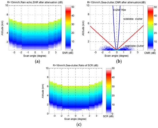
Figure 6.
The power ratio of the rain echo signal to noise (SNR), the power ratio of clutter signal to noise (CNR) after rain attenuation, and the power ratio of the rain echo signal to clutter signal (SCR). A uniform stratiform rain layer is assumed with the rain top of 6 km; (a) SNR of rain intensity at 10 mm/h; (b) CNR of the sea surface; and (c) SCR of the sea surface greater than 0 dB.
Usually the SCR with 0 dB is used as the minimum threshold to indicate whether the clutter interference will be serious [7,8,9,10]. In addition, GSWR will work at Ka-band, so the rain attenuation is much more serious. Different rain intensity will cause different rain attenuation, and it will finally lead to different SCR values. In the following sections, we calculated the SCR value from the sea surface clutter of media-intensity (wind speed: 10–15 m/s, NRCS from APR2) and the land surface of forest (Amazon rainforest) and desert (Libyan Desert), and use these results to evaluate the extension of clutter interference for GSWR.
Figure 7 shows the SCR results between the sea surface clutter and four types of different rain intensity. Only those SCR results below 0 dB are shown in these figures, which can directly indicate the scan angles and the height interfered by surface clutter in GSWR. Results indicate that the regions of surface clutter interference are wide when the rain intensity is 1 mm/h or less. As the rain intensity increases to 5 mm/h, the rain echoes are mainly interfered by the antenna mainlobe. The maximum interfered angles are centralized on 1° to 2° and its interfered height is close to 1.5 km. However, when the rain intensity increases to 10 mm/h or greater, the rain echoes, except those at nadir, are slightly affected by sea surface clutter due to significant rain attenuation. Certainly, the rain echoes near the sea surface are also attenuated significantly.
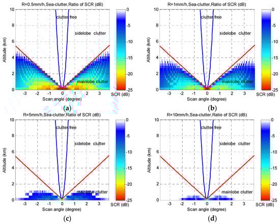
Figure 7.
Power ratio of rain echo signal to sea surface clutter (SCR) with middle wind-speed of 10–15 m/s (NRCS data from APR2), under different spiral scan angles and different rain rates. The figures only show those SCR values below 0 dB; (a) 0.5 mm/h; (b) 1 mm/h; (c) 5 mm/h; and (d) 10 mm/h.
Due to rain attenuation, the clutter regions of SCR less than 0 dB from the land surface are much smaller than those from the sea surface. Figure 8 shows the SCR results under rain intensities of 1 mm/h and 5 mm/h. Results show that the rain echoes interfered by the land surface clutter are mainly from the antenna mainlobe when the rain intensity is about 1 mm/h. However, when the rain intensity increases to 5 mm/h or greater, the rain echoes, except for those at nadir, are slightly affected by land surface clutter.
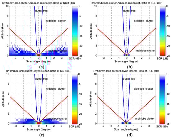
Figure 8.
Power ratio of rain echo signal to land surface clutter (SCR), with land terrain of Amazon rainforest and Libyan Desert. (a) SCR: 1 mm/h, Amazon rain forest; (b) 5 mm/h, Amazon rain forest; (c) SCR: 1 mm/h, Libyan desert; and (d) 5 mm/h, Libyan desert.
From the SCR between rain echo and sea surface clutter and land surface of forest and desert terrain above, we can easily determine that the SCR of other types of land surfaces and sea surfaces. In brief, due to rain attenuation, the GSWR will not be interfered with by sea surface and land surface clutter when the rain intensity is greater than 10 mm/h when its scan angles deviate from nadir.
3.3. The Effect of Attenna Mainlobe Width and Sidelobe Level to Clutter
The antenna main lobe and sidelobe are the most important methods to cause surface clutter interference to rain echoes for GSWR, where the interfered regions and extension are determined by the antenna main lobe and sidelobe. As we know, these two parameters usually decide the total cost and difficulty of antenna design. Here, the performance needs of the antenna main lobe and sidelobe are expected to be analyzed from the view of surface clutter interference. We hope these can provide helpful results for the antenna design in implementing GSWR. In these calculations, we obtain the different antenna main lobe and sidelobe through adjusting the Taylor weighting function and the antenna diameter.
Figure 9 has given the clutter power distribution of the sea surface with a wind speed of 10–15 m/s from two different antenna beamwidth, where the antenna sidelobe is −30 dB. Figure 4f shows the similar clutter power distribution with the antenna beamwidth of 0.02°. As shown in these three figures, we can see that the antenna beamwidth will affect the height and the power of clutter interference. The height of clutter interference will be gradually higher with the increase in the antenna beamwidth. When the beamwidth changes from 0.02° to 0.03°, the height of clutter interference close to the maximum scan angles has increased 2 km. The reason is that the cross intersectional area between the antenna beam and the Earth’s surface increased with a wider beamwidth, which finally decided the height of clutter interference. However, the power of these increased clutters is weaker than –100 dBm. In addition, the whole powers of clutter in the larger beamwidth will decrease slightly. When the antenna beamwidth changes from 0.02° to 0.03°, the power of clutter close to sea surface will reduce from 2 dB to 5 dB. This is because the wider beamwidth means the smaller size and the lower gain of the antenna. Obviously, if rain attenuation is considered, especially when the rain intensity is greater than 5 mm/h, the extension of clutter interference will not be affected by changing the beamwidth from 0.02° to 0.03°.
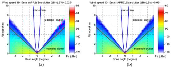
Figure 9.
Power distribution (dBm) of sea clutter under different beamwidths where wind speed is 10–15 m/s. The data of NRCS is measured by APR2. (a) Beamwidth (BW): 0.025°; and (b) beamwidth (BW): 0.03°; Figure 4c ahead has shown the similar calculation with a beamwidth (BW): 0.02°.
Figure 10 shows the clutter power distribution of the sea surface from two different antenna sidelobes, where the antenna beamwidth is 0.02°. Theoretically, the height of clutter interference will be gradually higher with the increasing of the antenna beamwidth. As shown in Figure 10a, the clutter power can be detected at the altitude of 10 km above due to the lower antenna sidelobe (SL = −15 dB). However, these clutter powers from the antenna sidelobe are much weaker compared with those from the antenna main lobe. The reason is that the two-way antenna weighting gain in the sidelobe is much weaker than that in main lobe. Comparing the power distribution in Figure 10b to those in Figure 4c, it can be easily found that the regions and the powers of the main lobe clutter do not have obvious changes when the antenna sidelobe decreased from −25 dB to −30 dB.
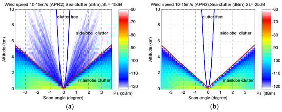
Figure 10.
Power distribution (dBm) of sea clutter under different antenna sidelobe, where wind speed is 10–15 m/s. The data of NRCS is measured by APR2. (a) antenna side lobe : SL = −15 dB; and (b) antenna side lobe: SL = −25 dB.
3.4. The Effect of Range Sidelobe Level to Clutter
Range sidelobe of pulse compression is also one of the most important ways to cause clutter interference in GSWR rain echoes. Usually, a lower range sidelobe will lead to less surface clutter interference. However, a lower range sidelobe means complex techniques for pulse compression, which will be determined by the complex design of the transmitting waveform and receiver matching filter.
Figure 11 has shown the clutter power distribution of a middle-intensity sea surface from four different range sidelobes. From the figures we can see that the powers of sea surface clutter from the range sidelobes are proportional to those from the antenna mainlobe and sidelobe, but the power of this clutter from the range sidelobe are obviously much weaker. With a range sidelobe of −40 dB, the height of clutter interference within the scan angle of 1° increased obviously, which can be up to 3.5 km. As shown in Figure 11d, when the range sidelobe reduces to −55 dB, the clutter powers from the range sidelobe near the surface shrink. If considering the rain attenuation, the clutter from the range sidelobe will be completely attenuated by rain echoes when the rain intensity is greater than 5 mm/h. In brief, the clutters from range sidelobes are weaker than those from the antenna mainlobe and sidelobe. The performance of range sidelobes with −55 dB can meet the need of design from the view of clutter suppression.
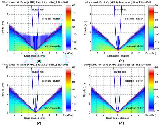
Figure 11.
Power distribution (dBm) of sea clutter under different range sidelobes, where wind speed is 10–15 m/s. The data of NRCS is measured by APR2. (a) range sidelobe: SSL = −40 dB; (b) range sidelobe: SSL = −45 dB; (c) range sidelobe: SSL = −50 dB; and (d) range sidelobe: SSL = −55 dB.
4. Conclusions
Aiming at the problem of surface clutter interference in future geostationary spaceborne weather radar, we introduce the producing principle of surface clutter from antenna mainlobe, sidelobe, and range sidelobe, and their methods of power calculation. Then those powers of different sea and land surface clutter with different scan angles are calculated, which are based on the parameters in the concept design of this radar system. By taking into account attenuation caused by rain, a signal-to-clutter ratio (SCR) is used to evaluate the extension of clutter interference. In addition, we change the parameters of antenna mainlobe, sidelobe, and range sidelobe, and reevaluated the variety of surface clutter interference, which can be expected to provide some performance reference for the future implementation of GSWR from the view of surface clutter suppression.
Numerical results show that the regions and extension of surface clutter interference in GSWR will be wider than those in TRMM PR. The maximum height of sea and land surface clutter will extend to 6 km. Most of clutter powers from sea and land surfaces at nadir are above −70 dBm, which are 50 dB greater than the minimum detectable power. If considering the rain attenuation to Ka-band electromagnetic waves, the regions and extension of clutter interference to GSWR will greatly decrease. When the rain intensity is 5 mm/h, the height of rain echoes interfered by sea surface clutter extends to 1.5 km, which are concentrated at angles of 1° to 2°, and rain echoes are not affected by land surface clutter when rain intensity is 5 mm/h or greater. If the rain intensity increases up to 10 mm/h, rain echoes, except for those near the surface at nadir, will be free from sea surface clutter contamination due to serious rain attenuation. Numerical results on changing the parameters of the radar antenna mainlobe, sidelobe, and range sidelobe also show that the surface clutter in GSWR will be caused mostly by the antenna mainlobe. With the increase of antenna beamwidth, the regions and extension of clutter interference will become wider than before. Reducing the level of the antenna sidelobe and range sidelobe to decrease the effects of clutter interference is not obvious. The performance of the antenna sidelobe less than –30 dB and the range sidelobe less than –55 dB can meet the needs of the radar system from the view of reducing surface clutter interference.
Acknowledgments
This work was supported by Natural Science Foundation of China (41475043, 41575022), Project of Sichuan Province (2014JY0093), Project of Chengdu University of Information Technology (KYTZ201414, J201601). The footprint pattern shown in Figure 1 was used from [4]. Partial equations of surface clutter calculation were cited from [7]. The authors are grateful to their help.
Author Contributions
X.L., J.H. conceived and designed the numerical experiments; C.W., X.H. designed the antenna pattern and range weighting function; X.L. performed the numerical experiments; X.L., J.H. and S.T. analyzed the results; X.L. wrote this paper.
Conflicts of Interest
The authors declare no conflict of interest.
References
- Lewis, W.E.; Im, E.; Tanelli, S.; Haddad, Z.; Tripoli, G.J.; Smith, E.A. Geostationary Doppler Radar and Tropical Cyclone Surveillance. J. Atmos. Ocean. Technol. 2011, 28, 1185–1191. [Google Scholar] [CrossRef]
- Tanelli, S.; Fang, H.; Durden, S.L.; Im, E.; Rahmat-Samii, Y. Prospects for geostationary Doppler weather radar. In Proceedings of the IEEE Radar Conference, Pasadena, CA, USA, 4–8 May 2009.
- Im, E.; Smith, E.A.; Chandrasekar, V.C.; Chen, S.; Holland, G.; Kakar, R.; Tripoli, G. Workshop Report on NEXRAD-In-Space—A Geostationary Satellite Doppler Weather Radar for Hurricane Studies. In Proceedings of the AMS 33rd Radar Meteorology Conference, Cairns, Australia, 6–10 August 2007.
- Im, E.; Smith, E.A.; Durden, S.L.; Tanelli, S.; Huang, J.; Rahmat-Samii, Y.; Lou, M. Instrument concept of NEXRAD In Space (NIS)—A geostationary radar for hurricane studies. In Proceedings of the Geoscience and Remote Sensing Symposium, Toulouse, France, 21–25 July 2003.
- Durden, S.L.; Tanelli, S. Application of clutter suppression methods to a geostationary weather radar concept. Prog. Electromagn. Res. Lett. 2009, 8, 115–124. [Google Scholar] [CrossRef]
- Okamoto, K.I.; Awaka, J.; Kozu, T. A feasibility Study of Rain Radar for the Tropical Rainfall Measuring Mission: Effects of Surface Clutter on Rain Measurements from Satellite. J. Commun. Res. Lab. 1988, 35, 183–208. [Google Scholar]
- Hanado, H.; Ihara, T. Evaluation of surface clutter for the design of the TRMM spaceborne radar. IEEE Trans. Geosci. Remote Sens. 1992, 30, 444–453. [Google Scholar] [CrossRef]
- Nepal, R.; Li, Z.; Zhang, Y.; Li, L. A simulation of study of the impact of surface clutter on spaceborne precipitation radar sensor. In Proceedings of the 36th Conference on Radar Meteorology, Breckenridge, CO, USA, 16–20 September 2013.
- Durden, S.L.; Im, E.; Li, F.K.; Girard, R.; Pak, K.S. Surface Clutter Due to Antenna Sidelobes for Spaceborne Atmospheric Radar. IEEE Trans. Geosci. Remote Sens. 2001, 39, 1916–1921. [Google Scholar] [CrossRef]
- Tagawa, T.; Okamoto, K.I.; Hanado, H.; Kozu, T. Suppression of surface clutter interference with TRMM precipitation radar observation. In Proceedings of the IEEE International Symposium on Geoscience and Remote Sensing, Denver, CO, USA, 31 July 2006.
- Tagawa, T.; Hanado, H.; Okamoto, K.I.; Kozu, T. Suppression of surface clutter interference with precipitation measurements by spaceborne precipitation radar. IEEE Trans. Geosci. Remote Sens. 2007, 45, 1324–1331. [Google Scholar] [CrossRef]
- Tagawa, T.; Okamoto, K.I. Calculations of surface clutter interference with precipitation measurement from space by 35.5 GHz radar for Global Precipitation Measurement Mission. In Proceedings of the IEEE International Geoscience and Remote Sensing Symposium, Toulouce, France, 21–25 July 2003.
- Durden, S.L.; Tanelli, S.; Meneghini, R. Using surface classification to improve surface reference technique performance over land. Indian J. Radio Space Phys. 2012, 41, 403–410. [Google Scholar]
- Yin, H.; Dong, X. Consideration of Antenna Pattern Design for FY3 Precipitation Measurement Satellite Dual-frequency Precipitation Radar. In Proceedings of the PIERS Proceedings, Xi’an, China, 22–26 March 2010.
- Yin, H.; Dong, X. Sea Clutter Analysis for Spaceborne Pulse-Compression Precipitation Radar. J. Nanjing Univ. Aeronaut. Astronaut. 2009, 41, 192–197. [Google Scholar]
- Ming, W. A ground clutter suppression method for 2D phased array spaceborne precipitation measurement radar. Mod. Radar 2009, 31, 23–27. [Google Scholar]
- Durden, S.L.; Tanelli, S.; Epp, L.W.; Jamnejad, V.; Long, E.M.; Perez, R.M.; Prata, A. System Design and Subsystem Technology for a Future Spaceborne Cloud Radar. IEEE Trans. Geosci. Remote Sens. Lett. 2016, 13, 560–564. [Google Scholar] [CrossRef]
- Kubota, T.; Iguchi, T.; Kojima, M. A Statistical Method for Reducing Sidelobe Clutter for the Ku-Band Precipitation Radar on board the GPM Core Observatory. J. Atmos. Ocean. Technol. 2016, 33, 1413–1428. [Google Scholar] [CrossRef]
- Ulaby, F.T.; Moore, R.K.; Fung, A.K. Microwave Remote Sensing Active and Passive-Volume II: Radar Remote Sensing and Surface Scattering and Enission Theory; Addison-Wesley Advanced Book Program: Reading, MA, USA, 1982; p. 609. [Google Scholar]
- Li, X.; He, J.; He, Z.; Zeng, Q. Geostationary weather radar super-resolution modelling and reconstruction process. Int. J. Simul. Process Model. 2012, 7, 81–88. [Google Scholar] [CrossRef]
- Zhang, L.; Yang, S.; Liu, J.; Lu, D. A method for retrieving inhomogeneous reflectivity fields within the radar beam. J. Remote Sens. 1998, 2, 81–89. [Google Scholar]
- Grant, C.R.; Yaplee, B.S. Back scattering from water and land at centimeter and millimeter wavelength. Proc. IRE 1957, 45, 976–982. [Google Scholar] [CrossRef]
- Satake, M.; Hanado, H. Diurnal change of Amazon rain forest σ 0 observed by Ku-band spaceborne radar. IEEE Trans. Geosci. Remote Sens. 2004, 42, 1127–1134. [Google Scholar] [CrossRef]
- Tanelli, S.; Durden, S.L.; Im, E. Simultaneous measurements of Ku-and Ka-band sea surface cross sections by an airborne radar. IEEE Trans. Geosci. Remote Sens. Lett. 2006, 3, 359–363. [Google Scholar] [CrossRef]
© 2017 by the authors; licensee MDPI, Basel, Switzerland. This article is an open access article distributed under the terms and conditions of the Creative Commons Attribution (CC-BY) license (http://creativecommons.org/licenses/by/4.0/).