Abstract
First continuous measurements of atmospheric CH4 were carried out for one year (June 2023–May 2024) at Liberti Observatory of CNR-IIA, in a semi-rural site near Rome. Seasonal and diurnal variations were analyzed. CH4 monthly mean concentrations showed maximum and minimum values in winter and summer, respectively, which agree with the other European trends. Minimum CH4 values during summer could likely be due to a combination of favorable atmospheric mixing properties and increased atmospheric CH4 oxidation. The correlation analysis showed that temperature, global radiation, and wind speed revealed significant negative correlations with this greenhouse gas, indicating the influence of local sources. However, poor correlations during different seasonal periods also suggested the role of air mass transport sources. The CH4 concentrations exhibited clear diurnal cycles with daytime low and night-time high values, mainly driven by atmospheric stability conditions and photochemistry. A cluster analysis of air mass trajectories showed that CH4 concentrations were influenced all year by anthropogenic emissions. Elevated concentrations arrived from NE Europe, except in winter when the influence of NW European and local contributions became more significant. Furthermore, level-3 XCH4 data from the satellite TROPOMI showed a methane columnar concentration increase from 2018 to 2024 in agreement with the global annual increase from the NOAA network during the same period.
1. Introduction
Methane (CH4) is the second most powerful greenhouse gas (GHG) after carbon dioxide (CO2) and a contributor to climate warming [1]. Global monthly mean concentrations were currently about 1927.61 ppb in July 2025, obtained from the Global Monitoring Division of NOAA’s Earth System Research Laboratory [2,3], showing an accelerating growth rate from late 2006, especially during the last years [4]. In 2006, the global annual mean was 1774.96 ppb, rising to 1929.97 in 2024 (a total rise of 155 ppb and a percentage difference of 8.73%). This increase is due principally to anthropogenic emissions, which contribute to about 60% of the total methane sources [5]. Although globally the sectors that contribute most to methane emissions are known, a better knowledge of the national situation is needed to support the policy maker in adopting measures that are as effective as possible. According to recent report of the National Greenhouse Gase Inventory 1990–2023 [6], CH4 emissions, in CO2 equivalent, represent 11.7% of total greenhouse gases in 2023 and are mainly originated from the agriculture sector which accounts for 46.1% of total methane emissions, as well as from the waste (40.9%), energy (12.9%), industrial processes, and product use (0.1%) sectors. Emissions in the agriculture sector regard mainly the enteric fermentation, manure management, rice cultivation and agricultural waste burning categories. Natural sources of methane include wetlands, freshwater systems, such as lakes, rivers, reservoirs, land geological sources, wildfire, termites and ruminant wild animals, permafrost and coastal and oceanic sources, and anaerobic decomposition of organic material [5].
The main sink of CH4 is its photochemical oxidation via tropospheric hydroxyl radicals (OH), making up about 90% of total CH4 oxidation [7] and leading to the CH4 tropospheric chemical lifetime of about a decade [8]. In addition, methanotrophic bacteria in soils, photochemical destruction in the stratosphere and oxidation via tropospheric chlorine radicals in marine environments [9] contribute to minor CH4 loss.
Methane is not only a significant contributor to global warming, but also directly affects air quality by increasing the concentration of tropospheric ozone (O3) [10]. Ozone itself is a GHG and a short-lived climate pollutant [1] impacting air quality, human health, vegetation, and ecosystems negatively [11].
Increasing atmospheric concentrations of greenhouse gases lead to global warming with adverse consequences, such as rising sea levels. It is, therefore, important to monitor the spatial distribution and temporal evolution of these gases and to improve our knowledge of their various natural and anthropogenic sources and sinks.
Thus, this study presents the first continuous in situ measurements, since June 2023, of a key greenhouse gas, such as CH4, at the Arnaldo Liberti Observatory, Institute of Atmospheric Pollution Research of the Italian National Research Council (CNR-IIA), located in Montelibretti Town near Rome (Italy). Being in central Italy (near Rome, Lazio), the Arnaldo Liberti Observatory extends the spatial coverage of the atmospheric national networks, located in northern and southern Italy. The observatory contributes significantly to our knowledge and provides useful information on observed methane variability and on its sources and sinks in the central Mediterranean Sea area and Europe. Indeed, the main objectives of this study are to explore the baseline levels, the daily and seasonal variability of atmospheric methane and evaluate the key drivers of this variability and its possible sources.
The meteorological parameters affecting pollutant concentrations at locale scale, integrated with a proxy to atmospheric mixing properties (such as radon progenies), combined with synoptic scale modeled backward trajectories, can provide an added value to the interpretation of the data collected. An effort to understand the different sources’ contributions, also based on a regional emission inventory, was made, giving a detailed insight into variations in methane concentration levels.
Further, a framing of the methane level in a broad area can be provided by satellite products. The SCanning Imaging Absorption spectroMeter for Atmospheric CartograpHY (SCIAMACHY) on board the European Space Agency’s environmental research satellite (ENVISAT, European Space Agency) [12] was the first space-based instrument designed to detect the near-surface concentration of atmospheric CH4 using the SWIR band. Later, the Greenhouse gases Observing SATellite (GOSAT, Japan Aerospace Exploration Agency), equipped with TANSO-FTS (thermal and near-infrared sensor for carbon observations-Fourier transform spectrometer), was able to retrieve CH4 [13] with higher sensitivity and spatial resolution than SCIAMACHY, and a low spatial sampling. Since 2018, the high accuracy and unprecedented temporal and spatial resolution and sampling of the TROPOspheric Monitoring Instrument (TROPOMI) on board the Copernicus Sentinel-5 Precursor (S5P, European Space Agency) satellite allows detailed and comprehensive overview of methane total column-averaged dry-air mole fraction (XCH4), i.e., the average fraction of CH4 molecules relative to total air molecules in the vertical column, on specific area of interest. To the aims of this study, the TROPOMI L3 products (PAL) are deemed suitable for a satellite frame of the annual trend of XCH4 over the last few years in the area where the Observatory is located.
2. Materials and Methods
2.1. Sampling Site: The Arnaldo Liberti Observatory
The Arnaldo Liberti Observatory (42°06′21″ N, 12°38′25″ E; 48 m a.s.l.) is a research infrastructure of the Institute of Atmospheric Pollution Research of the Italian National Research Council (CNR-IIA) inside the Research Area of Rome 1 (ARRM1) in Montelibretti (Rome, Italy). It is a semi-rural site in the Tiber Valley, about 30 km northeast (NE) of the Rome urban area, about 60 km NE of Fiumicino town, about 45 km NE of the Tyrrhenian Sea, about 5 km west southwest (WSW) of Monterotondo town, and about 2 km west (W) of heavy traffic roads. This study area is often affected by local emissions due to agricultural activities surrounding the Observatory, livestock farming areas (the nearest one hosting about 800 animals), biomass heating and traffic sources, and by transport of air masses from the urban area of Rome due to sea-breeze circulation [14]. This site is an EMEP station (Co-operative Programme for monitoring and evaluation of the long-range transmission of air pollutants in Europe), chosen as representative for monitoring of the transport and transformation of atmospheric pollution generated in the urban area of Rome.
The location of the site investigated, on the eastern bank of the Tiber River, with the peculiar geomorphological setting described in Marra et al., 2019 [15], does not seem to affect the background levels of methane, since in this stretch of the river, no emissions, both biogenic and abiogenic, are reported in the literature [16,17,18]. Conversely, along the Tiber Valley, carbon dioxide vents are well documented in the northern part (Alto tiberina) [19], in the middle part [20] and further down, in the lower part at Prima Porta [21]. At the end, toward the delta of the Tiber River and after passing through Rome downtown, methane emissions have been observed [22].
2.2. In Situ CH4 Measurements
Methane concentration was measured continuously from June 2023 to May 2024 by using a Picarro G2311-f analyzer (Picarro, Inc., 3105 Patrick Henry Dr., Santa Clara, CA 95054, USA) based on the Cavity Ring-Down Spectroscopy technique (CRDS) [23]. The analyzer was made available by CNR-IRET (Research Institute on Terrestrial Ecosystems), which also provided the technical support concerning routine operations, maintenance, and data handling. The CH4 analyzer was periodically calibrated and tested. Routine maintenance was performed, and the instrument underwent regular remote inspections by company technicians to ensure accuracy and long-term stability. Specifically, the Picarro calibration was checked weekly using a 10 L cylinder containing a 10-ppm methane mixture in nitrogen and a cylinder containing 402 ppm of CO2 in air (both supplied by S.I.A.D. S.p.A., Bergamo, Italy). The instrument simultaneously measures CO2 and H2O concentrations and applies automated water-vapor corrections [24], reporting dry-air mole fractions in ppm. Hourly means were calculated for seasonal, diurnal, and weekly analyses.
Air was sampled through a ¼″ Teflon FEP tube from the roof of the Arnaldo Liberti Observatory, with a 1 µm PTFE filter at the inlet to prevent dust contamination. The analyzer was operated in “high-precision” mode using a low-flow adapter, as recommended by the manufacturer for localized flux measurements over extended periods.
Data were recorded with the CRDS Data Viewer g2000-1.8.1.12 software at 0.4 s intervals. The instrument was factory-calibrated and underwent regular remote checks by company technicians to ensure accuracy and long-term stability. The precision is ≤150 ppb for CO2, ≤1 ppb for CH4, and ≤6 ppm for H2O. The operating ranges are 0–1000 ppm for CO2, 0–20 ppm for CH4, and 0–7%v for H2O.
The Picarro data were processed using MATLAB 2023b, and periods corresponding to regular maintenance operations were discarded.
2.3. Ancillary Measurements
Along with CH4, the continuous and simultaneous measurements of other gases, such as ozone (O3), nitrogen oxides (NOx, NO and NO2), and formaldehyde (HCHO), were also carried out during the same sampling period.
O3 measurements were conducted using the UV absorption O3 analyzer (Model T400 Teledyne API, Project Automation SpA, Monza, MB, Italy) The O3 measurements determine ozone concentration by measuring the absorption of UV light at 254 nm by the ozone molecules in sampled air and then using the Beer-Lambert law. The lower detection limit is less than 0.4 ppb, and the measurement precision is 0.5%. This technique is a European Air Quality standard [25] method for measuring atmospheric ozone.
Nitrogen oxides were monitored using a NOx analyzer (Model 200A Teledyne API, Teledyne Instruments, San Diego, CA, USA), based on the chemiluminescence reaction of NO with O3 to form electronically excited NO2. This molecule can decay by light emission of wavelengths between 600 and 3000 nm, with a peak at about 630 nm. Intensity of light emission is linearly proportional to the concentration of NO. The lower detection limit of the instrument is 0.4 ppb, and the measurement precision of 0.5%. This technique is a European standard method for measuring atmospheric nitrogen oxides [26].
The O3 and NOx analyzers were periodically calibrated and tested for air quality control using standards traceable to NIST. These measurements and other measured variables (such as PM10 and PM2.5) contribute to the EMEP Programme (Co-operative Programme for Monitoring and Evaluation of the Long-range Transmission of Air Pollutants in Europe), being the Arnaldo Liberti Observatory, a level 1 EMEP site.
Formaldehyde (HCHO) concentrations were measured continuously with the AL4021 HCHO analyzer (Aero-Laser GmbH, Garmisch-Partenkirchen, Germany), having a detection limit of 100 ppt (two times the standard deviation of the AL4021 instrument zeros by the manufacturer). This instrument is based on the Hantzsch reaction with fluorescence detection around 510 nm [27]. More technical details, operation protocols, field, and laboratory investigations of this instrument are available elsewhere [28,29,30]. Calibrations to assess the sensitivity of the instrument, as well as the measured flow rates, procedures, and baseline instrument, were periodically performed.
Natural radioactivity has been measured by means of a stability monitor (PBL Mixing Monitor, FAI Instruments, Fonte Nuova, Rome, Italy), which samples the atmospheric particulate matter where the short-lived Radon progeny fixes. A Geiger–Muller counter determines the natural radioactivity level (counts/min) on an hourly basis. Radon emissions vary according to soil composition and physical characteristics and can be considered rather spatially and temporally constant for the observations [31,32]. Thus, Radon decay products emission rates mainly depend on the dilution factor and can be considered as natural proxies of the mixing properties of lower atmospheric layers [33,34,35]. The monitoring of natural radioactivity can improve the characterization of the entire study period in terms of pollutants’ dispersion and/or emission from local sources.
In addition, meteorological measurements were obtained by a conventional meteorological station (Lsi Lastem s.r.l., Milan, Italy), consisting of a two-meter height mast mounted on the roof of a shed structure at the Liberti Observatory, reaching a total height of about 5.5 m a.g.l. This station is equipped with sensors for air temperature, relative humidity, pressure, and global solar radiation. Wind speed and wind direction were measured by a sonic anemometer (DMB305, Lsi Lastem s.r.l., Milan, Italy), positioned on a ten-meter mast near the meteorological station. All sensors were connected to a datalogger, acquiring and storing the collected data in real time.
All data collected from the three analyzers and the meteorological station were averaged over 5 min intervals, and their quality was guaranteed by discarding concentrations lower than their detection limits as well as noisy data and sharp spikes.
For seasonal evaluation, all data were grouped as follows: MAM = March, April, May for spring; JJA = June, July, August for summer; SON = September, October, November for autumn; and DJF = December, January, February for winter.
Comprehensive data processing, including quality control and wind patterns, was performed by IGOR Pro (WaveMetrics, Inc., Lake Oswego, OR, USA), whereas the openair package in R [36] was employed for statistical analysis and derived metrics.
2.4. Emission Sources
Methane emissions at the Liberti site can originate from various anthropogenic activities, namely agriculture, waste management and the energy sector, as well as natural sources. A local emission inventory is not available. However, local methane emission trends can be partially deduced from the most recent emission inventory provided by the Regional Environmental Protection Agency (ARPA Lazio) [37]. Different from previous inventories, in this last analysis, the share of methane recovered in landfills through biogas capture and combustion (in energy recovery plants or in flares) was deducted, improving the accuracy of the inventory.
At the regional (Lazio) level, the largest contribution comes from waste treatment and disposal (49% with approximately 59,500 Mg). The Rome metropolitan area near the Liberti site hosts some landfills and wastewater treatment facilities, which are notable sources of methane emissions, influencing the atmospheric composition at the Liberti site. Agriculture is the second largest methane source in Lazio (23% with approximately 28,000 Mg). The Liberti site, located in the Tiber Valley encompassing Montelibretti, is characterized by the presence of livestock farming, significantly contributing to local methane emissions through both enteric fermentation and manure management. Other sources of methane in Lazio are non-industrial combustion plants (20% with approximately 25,100 Mg) and the extraction and distribution of fossil fuels (6% with 7300 Mg). Furthermore, in Fiumicino town, located along the Tyrrhenian coast and about 30 km SW of Rome, in the Tiber River Delta and near the international airport, there is an active Sediment-Hosted Geothermal System (SHGS), a significant natural source of atmospheric geothermal CO2 and biotic CH4 [16,22,38,39,40]. Moreover, the Colli Albani volcanic system contains natural degassing zones (e.g., Tivoli, Tor Caldara of Lavinio, Solforata of Pomezia, Cava dei Selci of Marino), which release significant concentrations of CO2, CH4, and H2S, especially in Cava dei Selci, about 20 km SE of Rome, and in Solforata, about 30 km SW of Rome [41,42].
Temporal variations in methane emissions cannot be obtained from the ARPA Lazio inventory, but trends at national (Italy) levels are available from the Global Methane Initiative (GMI) database [43], where sources are classified in other emission sectors (biogas, coal mines, oil and gas, other), which are different from those used in the ARPA inventory. However, there is good agreement between the two inventories. In the GMI inventory, “other” sources, including waste management, are the major emitters, followed by “biogas” (e.g., agriculture) and oil and gas, including non-industrial combustion. Based on such an agreement, temporal variations in GMI emissions at the national level can be used as a reliable indicator of temporal variation for the Liberti site. These variations are reported in Figure 1. Methane emission form all sectors have slightly increased in the 1990s and then rapidly decreased in the 2000–2015 period, finally continuing a slight decrease in 2015–2024. The stronger percentage reduction is observed in the oil and gas sector, which includes non-industrial combustion plants. On the other hand, the most impactful reduction is associated with the biogas/agriculture sector.
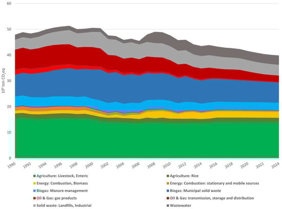
Figure 1.
Methane temporal emission trends by sectors in Italy [43].
2.5. TROPOMI L3 Products
The TROPOspheric Monitoring Instrument (TROPOMI) was launched onboard the European Space Agency’s (ESA) Sentinel-5 Precursor satellite in October 2017, with a near-polar sun-synchronous orbit, assuring a daily acquisition at 13:30 local solar time [44]. The methane total column-averaged dry-air mole fraction (XCH4) is retrieved from the spectral measurements of the SWIR spectrometer with a spectral resolution of 0.25 nm and a spectral sampling of 0.1 nm by applying the RemoTec algorithm [45,46,47], previously customized for OCO-2 and GOSAT measurements [48,49].
The TROPOMI–PAL reprocessed data [50], available from 2018 to 2024, are appropriate for the local yearly CH4 trend analysis. The L3 gridded data products are generated from operational Sentinel-5P L2 products by Sentinel 5P processors running in S5P-PAL service based on the HARP toolset [51].
To assess the regional variation in CH4 and possibly identify trends in the Liberti Observatory surroundings or local emission sources, the temporal and spatial variability of methane was investigated in a study area partially covering the Lazio Region. The study area (SA) includes two sub-areas on which statistical analysis was performed: the Tiber Valley (TV), following the Tiber River Basin and including the Liberti Observatory and the urban area of Rome (RM). The area of Rome was investigated because it represents a possible emitting source able to influence the Tiber Valley values. Differences between 2024 and 2018 (DIFF24−18) were obtained by applying the following equation:
where ‘x’ represents methane concentration (ppb) in each pixel. The delta map was used to visualize temporal changes. The annual means of methane emissions in the study area and the two sub-areas were then calculated to quantify changes over time.
2.6. HYSPLIT Backward Trajectories and Cluster Analysis
Backward trajectories are commonly used to identify the origin and transport patterns of air parcels, which influence air pollution concentrations at specific locations. Backward trajectories were calculated using the HYbrid Single-Particle Lagrangian Integrated Trajectory model (HYSPLIT) developed by NOAA Air Resources Laboratory (ARL) [52]. The HYSPLIT model is designed to calculate air parcel trajectories and perform complex simulations of transport, dispersion, chemical transformation, and deposition. The model employs a combination of Lagrangian and Eulerian methods and has been successfully utilized to study air mass transport, as well as dispersion and deposition of pollutants [53,54,55,56].
In this work, 96-h back trajectories were calculated from Liberti Observatory every hour for the entire record period. Altitude, latitude, and longitudes of the air parcel were calculated at 1 h intervals, starting at 50 m (above ground level), using the meteorological dataset GFS (Global Forecast System), with 0.25-degree horizontal resolution from the NOAA-Air Resources Laboratory.
The back trajectories were post-processed using HYSPLIT clustering analysis [52,57,58]. With this technique, trajectories near each other can be grouped into clusters and represented by their mean trajectory, and the error in the individual trajectories tends to balance out [59].
Optimal groupings were identified using the Total Spatial Variance (TSV) criterion, implemented in the HYSPLIT clustering module. Within this framework, cluster spatial variance (CSV) is evaluated by computing the total distances between individual trajectory endpoints and their corresponding cluster mean trajectory, and the TSV is then obtained as the sum of all cluster CSVs. The number of clusters suitable for this study was selected using the ‘elbow’ criterion, at the point where adding clusters produced only a small decrease in TSV, while avoiding the inclusion of dissimilar trajectories within the same cluster [60]. Hourly averages of methane mixing ratios associated with the trajectories of each cluster were computed. Subsequently, five-number statistical summaries were derived for each cluster and compared to evaluate differences in cluster behavior and to assess the influence of prevailing synoptic-scale air mass patterns on methane mixing ratios at the sampling site [61].
Back-trajectory analyses were performed using the ZeFir toolkit implemented in Igor Pro [61].
3. Results and Discussion
3.1. Meteorological Conditions
Meteorological parameters largely contribute to variations in diurnal and seasonal concentrations of air pollutants and play an important role in atmospheric chemical reactions. However, the magnitude of meteorological influences depends on the geographical location of the emission source and the type of pollutants. Table 1 presents the monthly mean values of the meteorological parameters, considering data every 5 min in the study period.

Table 1.
Monthly averages with standard deviations of temperature (T), relative humidity (RH), wind speed (WS), pressure (P) and global radiation (GR), and total monthly precipitation (Rain) from June 2023 to May 2024 at Arnaldo Liberti Observatory.
During the study period, the air temperature (T) showed a seasonal trend of high values in summer, with maximum values of 41.58 °C in July 2023 and low values in winter, with a minimum value of −1.82 °C in January 2024. The same trend was observed for global radiation (GR), which increased from winter to summer with maximum values of 1323.22 W/m2 in August 2023. Regarding the relative humidity (RH), this parameter showed lower levels in summer, especially in July 2023, when a minimum value of 17.07% was observed. The total precipitation (rain) over the whole study period was 860.40 mm, with a maximum total monthly value recorded during autumn and spring periods (November 2023 and March 2024), while the minimum total monthly precipitation was observed in September 2023. Referring to atmospheric pressure (P), it exhibited minimal temporal variations with a minimum value of 991.42 mbar in August 2023 and a maximum value of about 1040.00 mbar in December 2023.
Wind speed (WS) remained almost constant throughout the whole study period, with an average value of 1.85 m/s, showing a predominance of calm wind, except for the autumn and winter periods when higher wind speeds were recorded. Particularly, a maximum value of 15.07 m/s was observed in November 2023. Figure 2 shows the wind roses grouped by season. In the summer of 2023, the prevailing wind directions were from north (N) and south–west (SW) (frequency of occurrence of 13.99% and 13.96%, respectively), but also the most frequent components from south (S) and WSW (frequency of occurrence of 10.72% and 9.79%, respectively). The southerly wind sectors were also associated with higher wind speeds. During the autumn of 2023, the north component persisted with a frequency of 17.89%, while the other most frequent wind directions were from south–east (SE), S, and E (frequency of occurrence of 13.99%, 12.68%, and 9.27%, respectively). The S wind sectors were also associated with higher wind speeds. The wind rose for winter 2023 showed that the predominant wind directions were N and SE (frequency of occurrence of 19.60 and 16.50%, respectively), associated with lower wind speeds. The other wind directions with higher frequency were from E and S (frequency of occurrence of 10.66 and 10.51%, respectively), associated with higher wind speeds. In spring 2024, the S, SW, N, and SE wind components prevailed with a frequency of 14.33%, 13.13%, 12.70%, and 11.89%, respectively. The southerly wind sectors were always associated with higher wind speeds.
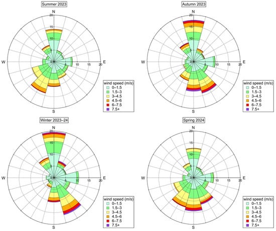
Figure 2.
Wind roses showing the frequency distributions of wind directions and speeds (color scale), grouped by season, averaged over the whole study period. The radius axis represents the occurrence from 0% to 20% for each season at Arnaldo Liberti Observatory.
In conclusion, the local wind circulation results in predominant N during all seasons and SE directions during winter and spring, while prevailing wind components from S-SW sectors occurred during spring and summer, with a persistence of the N component even if with lower speed than in summer and spring. Winds from the south–west direction are due to sea breeze, which easily develops in this sampling site and transports anthropogenic emissions of the urban area of Rome [14], while the other wind components could indicate local sources, identified earlier (Section 2.1 and Section 2.4), near the sampling site. These results are consistent with previous studies carried out at the observatory [30,62].
3.2. Monthly and Seasonal Variations
During the whole study period, the monthly CH4 concentrations ranged from 1.95 ± 0.05 ppm to 2.29 ± 0.05 ppm (Table 2) with a total average value of 2.05 ± 0.05 ppm, which were higher than global monthly and annual mean data observed from the NOAA network for the same periods, suggesting local emission impact on the concentrations observed at the sampling site.
Table 2.
Basic statistical parameters calculated on hourly means collected monthly at Arnaldo Liberti Observatory (June 2023–May 2024).
As shown in Table 2 and Figure 3, the seasonal variations in CH4 exhibited maximum monthly mean concentrations during winter, especially in December 2023, and minimum values during summer, particularly in July 2023. This seasonality and, thus, the decrease in concentrations detected in warm periods are due to concurrent favorable events, such as increased atmospheric mixing and a more efficient oxidation process of CH4 driven by the hydroxyl radical (OH) [63,64,65,66], which is photochemically produced and varies seasonally with available solar radiation reaching its maximum values in summer [67]. This seasonal trend agrees with the northern hemisphere seasonality of atmospheric methane oxidation [68,69] as well as the absence of heating emissions in warm periods, as also observed in other studies [63,64,70,71,72]. However, an additional second, smaller peak was observed during the spring, especially in April 2024. It could be attributed to local sources from agricultural activities that are expected to be larger in this period for the growing season after the rainy period. This monthly evolution was consistent with the trends reported in other European sites in Italy [63,65,73], Spain and the Iberian Peninsula [74,75], Central Europe [76], and the other sites of the northern hemisphere [69].
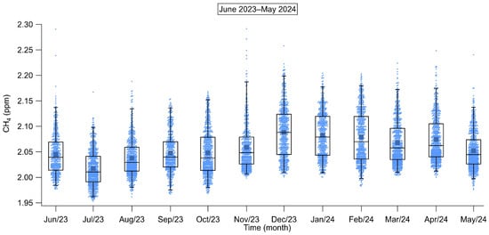
Figure 3.
The box and whisker plots (with individual data points) of monthly mean CH4 concentrations at Arnaldo Liberti Observatory. The top and the bottom of each box represent the 75th and 25th percentiles, respectively, and the upper and lower whiskers represent the 98th and 2nd percentiles. The horizontal bar in each box represents the median, and the square represents the mean value.
The influence of meteorological parameters on monthly CH4 concentrations was examined by performing linear regression analyses and calculating Pearson correlation coefficients (R) with a significance level (p-value < 0.05). The results, shown in Table 3, indicated that air temperature showed significant negative correlations with CH4 across all months, with R values exceeding −0.70 during the winter (December 2023 and January 2024), and −0.60 during the summer (July 2023). A negative correlation between methane and global radiation was also observed, although it was significant only in some months, especially during summer. Thus, the effect of global radiation and temperature, with the combination of methane removal by OH, regulated the seasonal levels of this gas at the observatory. Furthermore, methane exhibited significant positive correlations with relative humidity in all sampling periods, with maximum R values reached during summer. The relative humidity dependence did not affect the concentrations during this season, which remained high anyway. The results highlight that temperature and incoming solar radiation play a key role with respect to relative humidity.
Table 3.
Pearson correlation coefficients for monthly CH4 concentrations compared with meteorological parameters across all months (p < 0.05).
A good negative correlation between monthly CH4 levels and wind speeds was also found, indicating the proximity of local sources near the sampling site. However, poor or absent correlations between CH4 and these meteorological parameters (T, GR, and WS) during different seasons suggested the role of both local and regional sources. To further detect the possible local sources, pollution roses of methane concentrations were calculated with wind speeds/directions for each season (Figure 4 and Figure 5). The results indicated that the highest CH4 levels appeared constantly under low wind speeds from northern wind directions in all seasons, especially in winter. Similarly, this occurrence of periodic moderate breeze from northern components was also observed previously at Liberti Observatory [62] and was associated with high NO2 concentrations in different seasons. However, another component from the SE direction was also associated with the highest CH4 levels and lower wind speeds, especially during winter and spring. This indicated that local sources (biomass burning, agricultural activity, and vehicular emissions) could exist. The lowest levels of this gas were also observed under higher wind speeds from S–SW wind directions, especially in spring, which can be attributed to atmospheric air mass transport of regional emissions far away from the sampling site.
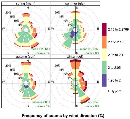
Figure 4.
Seasonal pollution roses of methane concentrations (ppm) with respect to observed wind directions at Arnaldo Liberti Observatory.
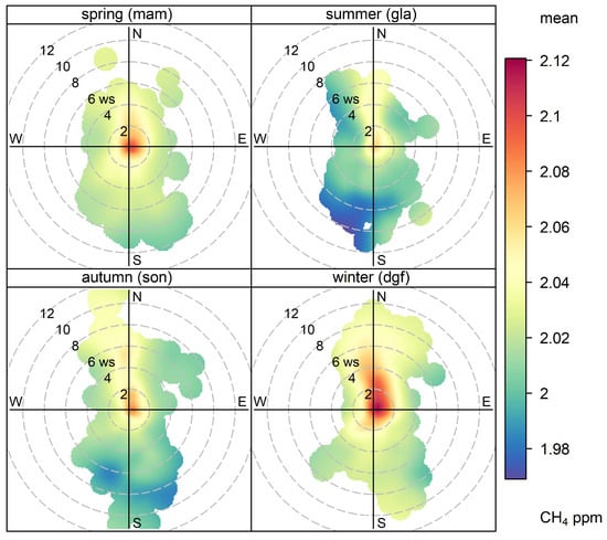
Figure 5.
Seasonal pollution roses of methane concentrations (ppm) with respect to observed wind speeds (m/s) and directions at Arnaldo Liberti Observatory.
These results suggest that the observed seasonal variations in CH4 concentrations were related to emitting sources, active sinks, and meteorological conditions throughout the year.
3.3. Diurnal Variations
Figure 6 shows the distinct CH4 daily cycles characterized by a night-time/early morning maximum, afternoon minimum, and a gradual increase through the evening until the next morning. The morning peak of CH4 concentrations occurred around 04:00–05:00 UTC in spring and summer, and about 05:00–06:00 UTC in autumn, before sunrise, which occurs after 05:00 and 06:00 UTC, respectively. In winter, this peak was delayed by 1–2 h in the morning when sunrise happened after 07:00 UTC. The morning peak could be due to the combined effect of the build-up of local anthropogenic activities (home heating and vehicular emissions) and seasonal sunlight changes. The decrease in CH4 concentrations during the daytime with respect to night-time levels was consistent with the atmospheric CH4 removal by the OH sink, which is formed mainly in the central hours of the day when the UV radiation is maximum, coinciding with higher air temperature during the day relative to the night. CH4 diurnal cycles also showed seasonal differences decreasing from winter to summer and increasing again during autumn.
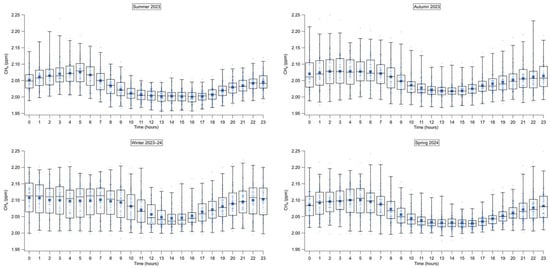
Figure 6.
The box and whisker plots (with individual data points) of hourly mean CH4 concentrations for each season at Arnaldo Liberti Observatory. The top and the bottom of each box represent the 75th and 25th percentiles, respectively, and the upper and lower whiskers represent the 98th and 2nd percentiles. The horizontal bar in each box represents the median, and the square represents the mean value.
These results indicated that diurnal cycles were mainly regulated by the reaction of CH4 with OH and meteorological conditions, such as solar radiation and air temperature.
Atmospheric Stability
The diurnal changes in atmospheric CH4 concentration in the sampling site were further examined, considering the influence of atmospheric stability conditions on this primary and low-reactive gas. Natural radioactivity due to Radon daughters can be considered a natural and reliable tracer to have information about mixing properties of the lower atmosphere and, thus, about atmospheric dispersion of air pollutants. Previous studies have shown that this measurement approach provides reliable information on boundary layer dispersion conditions [34,35]. Indeed, unreactive primary pollutants, such as CH4, are mainly modulated by both source strength and stability conditions, while secondary pollutants are more reactive, and their concentrations also depend on complex atmospheric formation and removal processes.
The daily variations in CH4 and natural radioactivity were very similar. The natural radioactivity levels showed a typical cyclic behavior in all seasons (Figure 7), exhibiting maximum values in early morning near the sunrise (around 04:00 UTC in spring and summer, around 05:00 UTC in autumn, and around 06:00 UTC in winter) in conditions of strong atmospheric stability and minimum values during the daytime when atmospheric mixing conditions occur. Subsequently, an increase in natural radioactivity began again in the late afternoon and lasted until the next day (nocturnal atmospheric stability) in all seasons. During the sunny hours, the solar heating of the atmosphere produces a well-mixed boundary layer favoring pollutant dilution and, thus, natural radioactivity values start to decrease from sunrise, reaching minimum levels during warm hours. Indeed, it is worth noting that the start of atmospheric mixing processes shifts from early morning in summer to late morning in winter. Conversely, during the night, precisely from sunset to sunrise, radiative cooling inhibits air mixing, leading to a stable atmosphere that suppresses the dispersion of pollutants. Thus, the natural radioactivity values are high. Thus, the accumulation of CH4 began in the afternoon during autumn and winter, and later in the evening during summer and spring. Further, significant positive correlations (p < 0.05) were observed between CH4 and natural radioactivity, with R values of 0.65, 0.71, 0.73, and 0.80 during the summer of 2023, the autumn of 2023, the winter of 2023, and the spring of 2024, respectively. This confirms that the daily CH4 concentrations followed and were consistent with the daily variations in natural radioactivity. During atmospheric stability conditions, the CH4 concentrations increased due to pollution accumulation from anthropogenic activities (such as household heating, in some cases through biomass-burning appliances, especially in winter, and vehicular transport) and then decreased during atmospheric mixing conditions (pollution dispersion) and increased photochemical destruction.
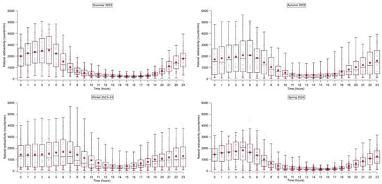
Figure 7.
The box and whisker plots (with individual data points) of hourly mean natural radioactivity counts for each season at Arnaldo Liberti Observatory. The top and the bottom of each box represent the 75th and 25th percentiles, respectively, and the upper and lower whiskers represent the 98th and 2nd percentiles. The horizontal bar in each box represents the median, and the square represents the mean value.
These results clearly indicated that atmospheric stability and its variations, which are linked to meteorological factors and to seasonal periods, were the main factors regulating the diurnal variations in atmospheric CH4 concentrations. Because this explained the observed daytime low and night-time/early morning high concentrations.
3.4. Weekly Variations
In addition to monthly and diurnal variations, the analysis of weekly trends (Monday to Sunday) could be useful to determine the possible influence of anthropogenic sources (industry, heating or transport activities) operating on a five-day working week (Monday to Friday).
The seasonal weekly trends of CH4 concentrations are shown in Figure 8. The results did not indicate a clear weekly variation in CH4 concentrations for all seasons, suggesting that no large anthropogenic sources of CH4 steadily affected its concentrations measured at the Arnaldo Liberti Observatory during working day periods, as also observed in Italian and other European sites [73,77,78].
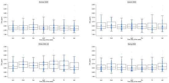
Figure 8.
The box and whisker plots (with individual data points) of weekly mean CH4 concentrations for each season at Arnaldo Liberti Observatory. The top and the bottom of each box represent the 75th and 25th percentiles, respectively, and the upper and lower whiskers represent the 98th and 2nd percentiles. The horizontal bar in each box represents the median, and the square represents the mean value.
3.5. Atmospheric Transport Impact on CH4
The influence of air mass transport of regional sources on CH4 levels at the sampling site was also investigated by using HYSPLIT clustering analysis computed with hourly mean concentrations of this gas. Back-trajectories were classified according to five different origins (Figure 9) for summer, autumn, winter, and spring. The main results are shown in Figure 10 and in Table 4 for each season and corresponding cluster.
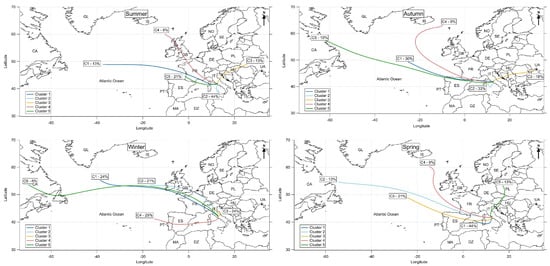
Figure 9.
Trajectory means the airflow patterns arriving at Arnaldo Liberti Observatory for each season during the course of a year. The percentages represent the frequency of occurrence for each cluster.
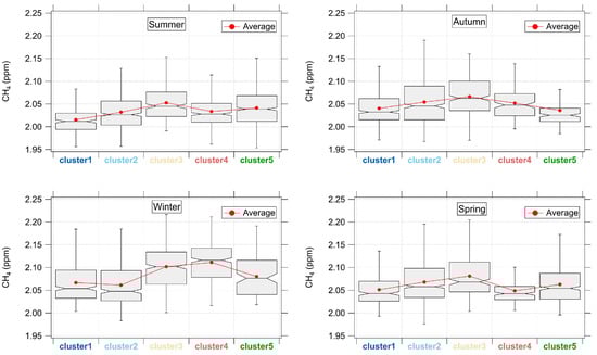
Figure 10.
The box and whiskers plots of methane concentrations for each cluster in each season. The horizontal line in each box represents the 50th percentile (median), the circle represents the mean value, the lower and upper boundaries locate the 25th and 75th percentiles of the values, and whiskers locate the minimum and maximum values that are not outliers. The different colors along x axis mean blue color for cluster 1, light blue color for cluster 2, yellow color for cluster 3, brownish red color for cluster 4 and green color for cluster 5 which are the same colors indicated for trajectories in Figure 9.
Table 4.
Seasonal clusters associated with median and mean CH4 concentrations and with air masses’ directions. The percentages in parentheses represent the frequency of occurrence for each cluster.
Along the backward trajectories, mixing of air masses of different origins occurs; some are impacted by both sea sources, with natural emissions and ship navigation [73,74], and land anthropogenic sources as described in the following. The marine sources, natural and anthropogenic, are affected by seasonality, and methane contribution from sea sources varies, depending on the trajectory characteristics and season, being to some extent less important during the cold seasons. Anthropogenic land sources are reported, considering the main literature findings, to provide a detailed overview of the possible origin of transported methane.
In summer, the Northern-Eastern (NE) European Cluster 3 showed the highest CH4 concentrations and lower occurrence frequency. Significant source contributions have been reported to originate from Croatia, Hungary, and Ukraine, with methane emissions from the oil and natural gas industry and production [79], from coal mining and war-related activities [80]. The second high concentrations were observed in Western (W) European Cluster 5, which was a slow air mass with high occurrence frequency. This cluster traversed the Balearic Sea and France in the western Mediterranean Sea, where methane emissions are primarily linked to both natural sources (wetlands and sediments) and anthropogenic activities (agriculture and wastewater treatment). The Balearic Sea is a CH4 source, even if a seasonal modulation with summer maxima was observed [81]. In addition to the sea-air flux, the contribution of shipping, particularly during touristic season, should also be considered. In the remaining part of the trajectory, France has significant methane source contributions mainly attributed to agricultural activities, with a maximum in summer [82]. The third high concentrations were found in the Northern-Western (NW) European Cluster 4 and in the local southern (S) Cluster 2, where the air masses were confined near the sampling site or its vicinity towards the Tyrrhenian Sea because they travelled short distances. Cluster 4 originated in the Atlantic Ocean, where maritime air would be cleaner, but then, it crossed the United Kingdom as well as France, which have agricultural activities and natural gas leak emissions [83]. Similar to Cluster 4, the methane levels associated with Cluster 2 could be due to dilution of cleaner maritime air, which originated from southern directions towards the Tyrrhenian Sea, with local air when the trajectories enter the Italian Peninsula and arrive at the sampling site. This local air corresponds to anthropogenic and natural sources from the urban city of Rome and its surrounding areas located in the southern sector of the sampling site (see Section 2.1 and Section 2.4). In the end, Cluster 1 is a fast air mass with low frequency and has its origin in the Atlantic Ocean from the west, inducing lower methane levels compared to the other clusters. During autumn, the highest mean CH4 concentrations remained linked to air masses from NE European regions (Cluster 3), where anthropogenic emissions could mainly originate from coal mining and oil production present in Romania [84]. The second high mean concentrations were observed in NW European (cluster 4) and in local SW directions (Cluster 2). Cluster 5 was associated with the lowest CH4 concentrations, likely due to the stronger marine character of the air masses coming from the W Atlantic Ocean directions compared to clusters 4 and 1. Furthermore, Cluster 1 crossed the Atlantic Ocean and the Balearic Sea and Spain in the western Mediterranean Sea, where methane emissions are primarily linked to both natural sources like coastal wetlands and sediments, and anthropogenic activities, particularly in the context of agriculture and wastewater treatment. The Balearic Sea behaves as a weak CH4 source [81] while the Ebro River Delta, located in the northern coasts of the Mediterranean Sea in Spain, is mainly covered by rice fields that could be a significant methane source, especially in late autumn and winter periods during the crop harvest period [85,86].
In winter, there were no trajectories from NE Europe, but the highest concentrations were transported from NW Europe (Cluster 4) and from local NW directions (Cluster 3). These clusters travelled across highly densely populated and industrialized regions, such as northern Italy (clusters 3 and 4), Switzerland, France, Belgium, and the UK (Cluster 4). Methane emissions in Northern Italy/Po valley are significant and come from agriculture (e.g., rice paddy fields, animal farming, and landfills) [87,88,89]. Further significant NW European contributions also originated from other regions (Switzerland, France, Belgium, and the UK) with intense agricultural and livestock activities, waste management, the energy sector, and leakages in the natural gas network. High concentrations were also found in the NW Atlantic Ocean directions, which traversed Canada (Cluster 5) with oil and gas industry, agriculture, landfills, and wetland emissions [90]. The remaining clusters, 1 and 2, were associated with lower CH4 concentrations compared to the other clusters since air masses from NW (Cluster 1) and SW (Cluster 2) directions were probably diluted with maritime air originating from the Atlantic Ocean.
In spring, the NE European directions (Cluster 3) reappeared and were associated with the highest concentrations. Indeed, this cluster moved over Poland (as well as Slovenia, Austria, and Czechia), which is the most significant source of coal mining methane levels in Europe, contributing to 41% of the total European coal emissions [91]. The other clusters with high CH4 concentrations were clusters 5 and 2 from the W and SW directions, respectively. Cluster 5 traversed the Atlantic Ocean, Spain, the Balearic Sea, and Sardinia, where waste and agriculture (rice and livestock sector) activities could make a significant contribution to CH4 levels [64,92]. Further, the local Cluster 2 traversed Sardinia, as did Cluster 5, beyond the Tyrrhenian and Balearic Sea. Sardinia Island holds the largest number of Italian farms rearing sheep, which is a significant source of methane emissions, accounting for 60% of the regional livestock greenhouse gases [93]. Finally, CH4 concentrations on the remaining clusters 1 and 4 were similar and lower due to maritime air originating from the W and NW Atlantic Ocean, respectively.
These results showed that CH4 concentrations at Liberti Observatory were influenced all year by anthropogenic regional emissions from NE Europe (oil and natural gas industry and production sources) in all seasons, except in winter when NW European and local contributions (agricultural and livestock activities, waste management, energy sector, and leakages in the natural gas network) became more significant with the highest CH4 levels observed at the sampling site. The remaining Atlantic and maritime trajectories generally reached the sampling site with the lowest CH4 levels.
3.6. Interrelation of CH4 (NOx, O3, HCHO)
CH4 is known to be one of the main precursors of HCHO, along with CH3CHO (acetaldehyde), CH3OH (methanol) and C5H8 (isoprene), and the patterns of reactions of formation (reported in detail in [94], connecting these species also involve the participation of OH, NO and intermediate radicals (CH3O2 and CH3O).
Both the formation of HCHO from CH4 and from C5H8 are dependent, respectively, on NO and NOx [95]. The methyl peroxynitrite intermediate (CH3OONO) further decomposes in CH3O and NO2, finally yielding HCHO and HONO (nitrous acid). Hence, a comprehensive treatment of the dataset is needed to understand the trends observed for the different pollutants.
Analyzing the monthly averaged data series of CH4 concentrations from June 2023 to May 2024, the expected seasonal variation, described in Section 3.4, was observed. Overall, the correlation of CH4 and HCHO was quite weak since Pearson correlation coefficients (R with p < 0.05) ranged from 0.01 in October 2023 to 0.34 in December 2023. A seasonal trend is evident, considering the correlation during hot and cold seasons. Negative values were calculated for the summer period, with R = −0.41. The strongest negative correlation was calculated for July 2023 (R = −0.39), whereas the strongest positive was found in December 2023 and February 2024 (R = 0.34). The negative correlation is likely related to the fact that in summer, the meteorological conditions promote atmospheric mixing as well as photochemical removal processes, such as the oxidation of CH4 by OH radicals with the formation of HCHO as an intermediate and CO2 as a final product. The almost equivalent positive correlation during winter, instead, points to the predominance of shared, common sources of the two pollutants. In other words, during summer, HCHO is mainly secondary, whereas in winter, direct emission is the predominant source.
The correlation among the different pollutants, i.e., CH4, HCHO, NO2, NO, and O3, was tested as well, and correlation matrices on a seasonal basis were obtained (details in Appendix A). There is always a negative correlation between CH4 and O3, with R Pearson coefficients (p < 0.05) ranging from R = −0.45 in September 2023 to R = −0.81 in March, whereas the correlation between O3 and HCHO changes with the season, being negative in winter, with the lowest value of R = −0.32 in December, and positive during summer with the highest value of R calculated for August data (R = 0.86). This finding is consistent with the secondary nature of the O3, while the mixed sources affecting HCHO mixing ratios, both primary and secondary, can explain the correlations found.
The anticorrelation between CH4 and O3 found throughout the period is due to several concurrent conditions, impacting the two species, which have different origins. Both are affected by atmospheric mixing properties, but their roles in photochemical processes are opposite, since CH4 decreases through oxidation processes, mainly triggered by the presence of OH radicals, whereas O3 is formed by methane and non-methane volatile organic hydrocarbons (NMVOCs) oxidation. This implies opposite diurnal trends of the two species. Since the nature of secondary pollution is complex and several different variables affect the formation/removal of pollutants, such as HCHO and O3, a comprehensive treatment of the dataset was performed through principal component analysis (PCA) (details in Appendix A). In Figure 11, the variables considered are reported with respect to the newly defined set of components. It can be observed that CH4, NO, and NO2 are always positively correlated, whereas HCHO is positively correlated with the three pollutants only during winter. In addition, a strong linkage between O3 and T, as reported by [96], can also be observed in Figure 11.
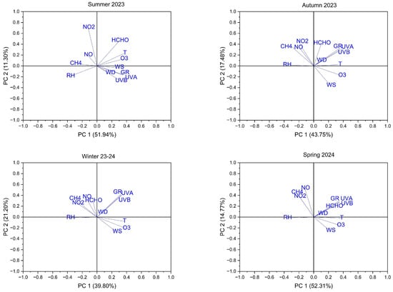
Figure 11.
PCA treatment on the seasonal datasets, comprehensive of pollutants data and meteorological parameters.
As expected, the photochemical production of HCHO is prevalent over primary emission, especially during summer, among the precursors, CH4 contribute is likely slightly enhanced with respect to winter or autumn, and, as reported previously in Section 3.2, a negative correlation was observed between global radiation and CH4 concentrations, likely due to the oxidation triggered by UV radiation.
This contribution is not easily accounted for, since only a small fraction of the CH4 is available for oxidation, given its low reactivity. Other organic precursors are predominant sources during this period (particularly isoprene and other terpenes).
By analyzing hourly average data, referred to UTC, over different seasonal daily cycles, reported in Figure 6 for CH4 and in Figure 12 for HCHO, it can be observed that, as expected, they show opposite trends. CH4 exhibits rather constant concentration values with night maxima in the timeframe 04:00–06:00, but this modulation is not present in the winter when only minimum values can be observed in the period 13:00–15:00. HCHO conversely is characterized by sharper maxima during daytime (09:00–12:00) in summer or spring, slightly shifted onwards during autumn (11:00–13:00), whereas during the winter evening maxima occurred from 17:00 to 20:00.
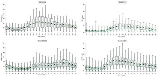
Figure 12.
The box and whisker plots (with individual data points) of hourly mean HCHO concentrations for each season at Arnaldo Liberti Observatory. The top and the bottom of each box represent the 75th and 25th percentiles, respectively, and the upper and lower whiskers represent the 98th and 2nd percentiles. The horizontal bar in each box represents the median, and the square represents the mean value.
The data collected allow for an evaluation of the photochemical reaction mechanisms leading to the formation of O3. The calculation of the HCHO/NO2 ratio is considered as a possible indicator of the main drivers to the formation of O3 [97], being 0.55 < HCHO/NO2 < 1, indicative of a condition of transition between a VOC-limited (HCHO/NO2 < 0.55) and a NOx-limited (HCHO/NO2 > 1) regime of formation. The values of the ratios calculated during spring–summer showed ratios higher than 1 for the months of July and August 2023 (1.18 and 1.34, respectively), and in 2024, this condition was present for the late spring in May with a ratio of 1.27.
Hence, as already observed in [30], the concentration of NOx is the limiting factor to the production of O3 at Liberti Observatory in late spring and summer.
3.7. Satellite-Framed Annual Trend
Figure 13 shows the temporal and spatial variation in CH4 in 2018 and 2024 at the regional level, considering a study area that includes the Liberti Observatory and the city of Rome and the two sub-areas (TV and RM). The difference map between the two years is also shown. Some pixels included in SA lack values, which is likely due to the strict filtering that is performed on L3 products’ quality assurance value (qa_value) [45,98]. Particularly, in mountain regions, complex terrain features, high albedo, and frequent cloud cover can interfere with the retrieval that falls below the quality threshold, leading to data gaps in the final product [45,98]. However, these pixels represent only a small fraction of the SA, and the satellite data are used to provide the regional and seasonal context for the in situ methane observations. Within this satellite-based assessment framework, the spatial pattern of missing pixels does not affect the interpretation of the results, as the area corresponding to the observatory is fully captured and unaffected by these data gaps.
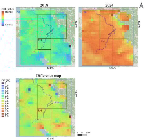
Figure 13.
The maps show the annual CH4 (ppbv) average in 2018 (left) and 2024 (right). The differences between 2018 and 2024 (down) are also shown. The Liberti Observatory (LibObs) is shown as a green spot, and the Tiber River is represented as a blue line. The SA area is delimited in light blue, the TV area in green, and the RM urban area in red. The figure includes the north arrow and the scale bar. The background map was obtained from OpenStreetMap Contributors (2024) [99].
The maps show a generalized increase in the whole region from 2018 to 2024, as 2024 clearly shows a higher range of values compared to 2018. The Liberti Observatory area always falls within the middle-lower values of the emission range. The delta map confirms this increase. Interestingly, the Liberti Observatory and the TV area follow the general trend of SA as RM, demonstrating that these subregions did not constitute a hotspot of methane columnar concentration increase. However, the analyzed maps may not be suitable for detecting locally minor emission sources, which cannot be resolved at the pixel scale. On the other hand, areas where the increase in methane columnar concentration was particularly intense are still recognizable in other regions of the SA (orange pixels in the difference maps). While natural emission sources are historically reported in the SA, they do not specifically correspond to orange pixels showing an increase in methane columnar concentration. Therefore, additional analysis would be needed to determine whether they are related to local emission sources of anthropogenic origin. The increase in methane concentrations s in the study area was confirmed by the temporal trends. Particularly, Figure 14 shows the continued increase in the CH4 detectable by L3 S5P-PAL products.
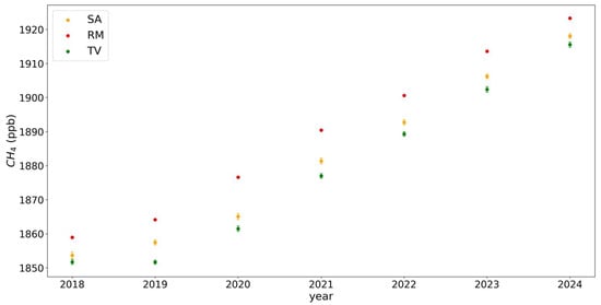
Figure 14.
Annual mean and uncertainty of CH4 emission in the study area (SA), in Rome (RM) and in the Tiber Valley (TV).
An increase of 3.45% in the southern part of the Tiber Valley has been inferred from satellite data over the last few years, while increases of 3.46% and 3.45% were detected on RM and TV, respectively. These results are statistically comparable. The temporal trend in the study area and in Rome confirms, indeed, that the increase was generalized, hence it is not associated with local hotspots in the Tiber Valley sub-region. This increase is in line with a general, global trend reporting an average for methane in 2017–2023 close to 1925 ppb [100]. Moreover, the Global Monitoring Division of NOAA’s Earth System Research Laboratory, which has measured methane since 1983 at a globally distributed network of air sampling sites, reported the global annual means of CH4 in 2018 and 2024, respectively 1857.34 and 1929.97 ppb. The rise was 72.63 ppb with a percentage difference of 3.91% [3]. The causes of this increase are unclear, but there is observation-based evidence tying anthropogenic fossil fuel use, agriculture, and waste management to the increase in the concentration of methane in the atmosphere. At the national level, methane emissions from residential buildings (i.e., due to domestic heating) nearly doubled between 2005 and 2020, specifically due to an increase in biomass combustion, which could explain the local increase [101].
4. Conclusions
The atmospheric methane measurements were carried out from June 2023 to May 2024 in a rural area near Rome (Lazio, Italy) at Arnaldo Liberti Observatory of the CNR-IIA.
This site can be considered representative of the immediate surroundings, since other semirural locations around the city of Rome are characterized by different environments, such as terrain reliefs, seaside proximity, etc.
Moreover, the data reported are limited to one year of observations, and only preliminary considerations concerning seasonal variations are reported in this work. Nevertheless, seasonal and diurnal variations in CH4 and associated meteorological parameters were analyzed. CH4 concentrations showed a typical seasonal monthly evolution, as observed in other European areas, with maximum and minimum values in late autumn-winter (December 2023) and summer (July 2023) periods, respectively. However, a secondary CH4 peak was also observed in April 2024, which could be attributed to agricultural activities in this rural area during the growing seasonal period. Further, minimum values during warm periods could be due principally to the atmospheric oxidation reaction of CH4 with OH, which has a seasonal maximum concentration in the northern hemisphere. The influence of meteorological parameters on the seasonal variation was investigated. CH4 was significantly and negatively correlated with local temperature, global radiation, and wind speed, indicating not only the importance of the temperature and solar radiation together with the atmospheric CH4 oxidation, but also the influence of local sources near the sampling site. Among different precursors, which would be the subject of specific future research, the CH4 contribution to the photochemical production of HCHO is significant during summer, and a negative correlation was observed between these two pollutants in this season.
With respect to local wind direction, CH4 showed the highest concentrations when the prevailing wind was from a northern direction in all seasons and from a southeastern direction during winter and spring periods in conjunction with low wind speeds. This behavior remarked on the influence of local sources on CH4 variations. Indeed, south and southwestern wind directions were associated with high wind speeds and high CH4 concentrations, especially during spring, indicating the possible effect of air mass transport of sources.
CH4 also showed a seasonal daily cycle with the highest values at night or early morning and the lowest during the afternoon, depending on the season. This pattern and the reduction in CH4 levels during the day compared to night or early morning highlight the role of atmospheric oxidation by OH, which mainly occurs during the central hours of the day. Additionally, the connection between daily CH4 variations and atmospheric stability was examined using the diurnal trends of natural radioactivity, which serve as a natural tracer for the mixing properties of the lower atmosphere. The results indicated that the diurnal cycle was primarily driven by atmospheric stability, linked to meteorological conditions and seasonal changes. This explains the observed higher CH4 concentrations at night and lower levels during the day. Furthermore, all these findings help clarify which local emissions and meteorological conditions lead to higher CH4 levels than the global average, causing deviations from global background concentrations. The evaluation of the influence of atmospheric regional transport on CH4 variations was also carried out using HYSPLIT clustering analysis computed with hourly mean concentrations of this gas. The results showed that CH4 concentrations at Liberti Observatory were influenced all year by anthropogenic regional emissions. Air masses originating from northeastern Europe were associated with the highest CH4 levels in summer, autumn, and spring, while in winter, northwestern European and local contributions became more significant. The remaining Atlantic trajectories generally reached the sampling site with the lowest CH4 levels.
Level-3 XCH4 data from the TROPOspheric Monitoring Instrument (TROPOMI) on board the Sentinel-5 Precursor satellite were used and aggregated into annual data. The results confirmed an increase of about 3.5% in methane emissions in the study area from 2018 to 2024, in agreement with the global annual increase of 3.9% in the same period observed by the Global Monitoring Division of NOAA’s Earth System Research Laboratory.
In conclusion, although CH4 is globally increased and distributed, its behavior and variability depend on the combined effects of several factors, such as local and regional sources, boundary layer dynamics, as well as meteorological conditions, and atmospheric oxidation, contributing to the observed concentrations throughout the year in a rural environment.
Author Contributions
Conceptualization, A.I. (Antonietta Ianniello), G.E. and E.P.; methodology, A.I. (Antonietta Ianniello), G.E., C.B., F.V., V.P., W.S., P.S., L.T., M.M., A.I. (Andrea Imperiali), A.I. (Alma Iannilli), V.T., P.T. and E.P.; software, G.E., C.B., F.V., W.S., P.S., L.T., M.M., A.I. (Alma Iannilli) and E.P.; validation, A.I. (Antonietta Ianniello), G.E. and E.P.; writing—original draft preparation, A.I. (Antonietta Ianniello), G.E., C.B., F.V., V.P., L.T. and E.P.; writing—review and editing, A.I. (Antonietta Ianniello), G.E., C.B., F.V., V.P., W.S., P.S., L.T., A.I. (Alma Iannilli), V.T., P.T. and E.P.; supervision, A.I. (Antonietta Ianniello) and G.E.; project administration, A.I. (Antonietta Ianniello), G.E. and E.P.; funding acquisition, A.I. (Antonietta Ianniello) and E.P. All authors have read and agreed to the published version of the manuscript.
Funding
This research received no external funding.
Data Availability Statement
Data are available upon request to the authors.
Acknowledgments
The authors would thank Marco Giusto (CNR-IIA) for the natural radioactivity data provided during the experimental activities. The authors have reviewed and edited the output and take full responsibility for the content of this publication.
Conflicts of Interest
The authors declare no conflicts of interest.
Appendix A

Figure A1.
Correlation matrix of pollutant concentration and meteorological parameters impacting photochemical pollution in summer 2023.
Figure A1.
Correlation matrix of pollutant concentration and meteorological parameters impacting photochemical pollution in summer 2023.


Figure A2.
Correlation matrix of pollutant concentration and meteorological parameters impacting photochemical pollution in autumn 2023.
Figure A2.
Correlation matrix of pollutant concentration and meteorological parameters impacting photochemical pollution in autumn 2023.


Figure A3.
Correlation matrix of pollutant concentration and meteorological parameters impacting photochemical pollution in winter 2023.
Figure A3.
Correlation matrix of pollutant concentration and meteorological parameters impacting photochemical pollution in winter 2023.


Figure A4.
Correlation Matrix of pollutant concentration and meteorological parameters impacting photochemical pollution in spring 2024.
Figure A4.
Correlation Matrix of pollutant concentration and meteorological parameters impacting photochemical pollution in spring 2024.

Table A1.
Percentual explained variances of the principal components obtained by PCA treatment on the datasets with different periods.
Table A1.
Percentual explained variances of the principal components obtained by PCA treatment on the datasets with different periods.
| Period | Component | Eigenvalue | % Variance | % Cum. Variance |
|---|---|---|---|---|
| summer 23 | 1 | 6.23 | 51.94% | 51.94% |
| 2 | 1.36 | 11.30% | 63.24% | |
| 3 | 1.29 | 10.78% | 74.02% | |
| autumn 23 | 1 | 6.00 | 50.00% | 50.00% |
| 2 | 1.68 | 14.03% | 64.02% | |
| 3 | 1.33 | 11.11% | 75.13% | |
| winter 23–24 | 1 | 4.77 | 39.80% | 39.80% |
| 2 | 2.54 | 21.20% | 61.01% | |
| 3 | 1.28 | 10.66% | 71.66% | |
| 4 | 1.00 | 8.38% | 80.04% | |
| spring 24 | 1 | 6.26 | 52.14% | 52.14% |
| 2 | 1.78 | 14.84% | 66.98% |
Table A2.
Loadings of the different variables to the principal components.
Table A2.
Loadings of the different variables to the principal components.
| Summer 23 | Autumn 23 | Winter 23–24 | Spring 24 | |||||
|---|---|---|---|---|---|---|---|---|
| PC1 | PC2 | PC1 | PC2 | PC1 | PC2 | PC1 | PC2 | |
| CH4 | −0.26 | 0.04 | −0.25 | 0.44 | −0.31 | 0.34 | −0.23 | 0.45 |
| HCHO | 0.30 | 0.46 | 0.27 | 0.34 | −0.06 | 0.30 | 0.27 | 0.20 |
| O3 | 0.36 | 0.13 | 0.36 | −0.10 | 0.39 | −0.21 | 0.36 | −0.15 |
| NO | −0.13 | 0.20 | −0.20 | 0.34 | −0.13 | 0.32 | −0.12 | 0.53 |
| NO2 | −0.12 | 0.71 | −0.19 | 0.39 | −0.27 | 0.25 | −0.19 | 0.38 |
| T | 0.37 | 0.23 | 0.36 | 0.01 | 0.36 | −0.08 | 0.37 | −0.02 |
| RH | −0.37 | −0.19 | −0.37 | −0.06 | −0.37 | −0.02 | −0.36 | −0.02 |
| GR | 0.35 | −0.16 | 0.33 | 0.30 | 0.32 | 0.42 | 0.34 | 0.29 |
| UVA | 0.36 | −0.17 | 0.35 | 0.27 | 0.33 | 0.40 | 0.35 | 0.27 |
| UVB | 0.32 | −0.28 | 0.32 | 0.19 | 0.33 | 0.40 | 0.35 | 0.28 |
| WS | 0.23 | −0.03 | 0.21 | −0.45 | 0.26 | −0.27 | 0.22 | −0.25 |
| WD | 0.12 | −0.09 | 0.13 | 0.01 | 0.07 | 0.08 | 0.12 | 0.06 |
References
- IPCC. Sections. In Climate Change 2023: Synthesis Report; Contribution of Working Groups I, II and III to the Sixth Assessment Report of the Intergovernmental Panel on Climate Change; Core Writing Team, Lee, H., Romero, J., Eds.; IPCC: Geneva, Switzerland, 2023; pp. 35–115. [Google Scholar] [CrossRef]
- Dlugokencky, E.J.; Steele, L.P.; Lang, P.M.; Masarie, K.A. The growth rate and distribution of atmospheric methane. J. Geophys. Res. 1994, 99, 17021–17043. [Google Scholar] [CrossRef]
- Lan, X.; Thoning, K.W.; Dlugokencky, E.J. Trends in Globally-Averaged CH4, N2O, and SF6 Determined from NOAA Global Monitoring Laboratory Measurements; Global Monitoring Laboratory: Boulder, CO, USA, 2022; Version 2024-02. [Google Scholar] [CrossRef]
- Nisbet, E.G.; Manning, M.R.; Dlugokencky, E.J.; Michel, S.E.; Lan, X.; Rockmann, T.; Denier van der Gon, H.A.C.; Schmitt, J.; Palmer, P.I.; Dyonisius, M.N.; et al. Atmospheric methane: Comparison between methane’s record in 2006–2022 and during glacial terminations. Glob. Biogeochem. Cycle 2023, 37, e2023GB007875. [Google Scholar] [CrossRef]
- Saunois, M.; Martinez, A.; Poulter, B.; Zhang, Z.; Raymond, P.; Regnier, P.; Canadell, J.G.; Jackson, R.B.; Patra, P.K.; Bousquet, P.; et al. Global Methane Budget 2000–2020. Earth Syst. Sci. Data 2025, 17, 1873–1958. [Google Scholar] [CrossRef]
- ISPRA. Italian Greenhouse Gas Inventory 1990–2023. In National Inventory Document 2025; Rapporti 398411/2025; ISPRA: Rome, Italy, 2025; ISBN 978-88-448-1252-2. Available online: https://www.isprambiente.gov.it/files2025/pubblicazioni/rapporti/nid2025_italy_stampa.pdf (accessed on 27 January 2026).
- Wang, Y.; Ming, T.; Li, W.; Yuan, Q.; de Richter, R.; Davies, P.; Caillol, S. Atmospheric removal of methane by enhancing the natural hydroxyl radical sink. Greenh. Gas. Sci. Technol. 2022, 12, 784–795. [Google Scholar] [CrossRef]
- Myhre, G.; Shindell, D.; Bréon, F.-M.; Collins, W.; Fuglestvedt, J.; Huang, J.; Koch, D.; Lamarque, J.-F.; Lee, D.; Mendoza, B.; et al. Anthropogenic and Natural Radiative Forcing. In Climate Change 2013: The Physical Science Basis; Contribution of Working Group I to the Fifth Assessment Report of the Intergovernmental Panel on Climate Change; Stocker, T.F., Qin, D., Plattner, G.-K., Tignor, M., Allen, S.K., Boschung, J., Nauels, A., Xia, Y., Bex, V., Midgley, P.M., Eds.; Cambridge University Press: Cambridge, UK; New York, NY, USA, 2013. [Google Scholar]
- Hossaini, R.; Chipperfield, M.P.; Saiz-Lopez, A.; Fernandez, R.; Monks, S.; Feng, W.; Brauer, P.; von Glasow, R. A global model of tropospheric chlorine chemistry: Organic versus inorganic sources and impact on methane oxidation. J. Geophys. Res. Atmos. 2016, 121, 14271–14297. [Google Scholar] [CrossRef]
- Fiore, A.M.; West, J.J.; Horowitz, L.W.; Naik, V.; Schwarzkopf, M.D. Characterizing the tropospheric ozone response to methane emission controls and the benefits to climate and air quality. J. Geophys. Res. 2008, 113, D08307. [Google Scholar] [CrossRef]
- Monks, P.S.; Archibald, A.T.; Colette, A.; Cooper, O.; Coyle, M.; Derwent, R.; Fowler, D.; Granier, C.; Law, K.S.; Mills, G.E.; et al. Tropospheric ozone and its precursors from the urban to the global scale from air quality to short-lived climate forcer. Atmos. Chem. Phys. 2015, 15, 8889–8973. [Google Scholar] [CrossRef]
- Bovensmann, H.; Burrows, J.P.; Buchwitz, M.; Frerick, J.; Noël, S.; Rozanov, V.V.; Chance, K.V.; Goede, A.P.H. 1999: SCIAMACHY: Mission Objectives and Measurement Modes. J. Atmos. Sci. 1999, 56, 127–150. [Google Scholar] [CrossRef]
- Kuze, A.; Suto, H.; Nakajima, M.; Hamazaki, T. Thermal and near infrared sensor for carbon observation Fourier-transform spectrometer on the Greenhouse Gases Observing Satellite for greenhouse gases monitoring. Appl. Opt. 2009, 48, 6716–6733. [Google Scholar] [CrossRef] [PubMed]
- Ciccioli, P.; Brancaleoni, E.; Frattoni, M. Chapter 5—Reactive Hydrocarbons in the Atmosphere at Urban and Regional Scales. In Reactive Hydrocarbons in the Atmosphere; Hewitt, C.N., Ed.; Academic Press: Cambridge, MA, USA, 1999; pp. 159–207. [Google Scholar] [CrossRef]
- Marra, F.; Florindo, F.; Jicha, B.R.; Nomade, S.; Palladino, D.M.; Pereira, A.; Sottili, G.; Tolomei, C. Volcano-tectonic deformation in the Monti Sabatini Volcanic District at the gates of Rome (central Italy): Evidence from new geochronologic constraints on the Tiber River MIS 5 terraces. Sci. Rep. 2019, 9, 11496. [Google Scholar] [CrossRef] [PubMed]
- Tassi, F.; Fiebig, J.; Vaselli, O.; Nocentini, M. Origins of methane discharging from volcanic-hydrothermal, geothermal and cold emissions in Italy. Chem. Geol. 2012, 310–311, 36–48. [Google Scholar] [CrossRef]
- Stanley, E.H.; Casson, N.J.; Christel, S.T.; Crawford, J.T.; Loken, L.C.; Oliver, S.K. The ecology of methane in streams and rivers: Patterns, controls, and global significance. Ecol. Monogr. 2016, 86, 146–171. [Google Scholar] [CrossRef]
- Stanley, E.H.; Loken, L.C.; Casson, N.J.; Oliver, S.K.; Sponseller, R.A.; Wallin, M.B.; Zhang, L.; Rocher-Ros, G. GRiMeDB: The Global River Methane Database of concentrations and fluxes. Earth Syst. Sci. Data 2023, 15, 2879–2926. [Google Scholar] [CrossRef]
- Caracausi, A.; Camarda, M.; Chiaraluce, L.; De Gregorio, S.; Favara, R.; Pisciotta, A. A novel infrastructure for the continuous monitoring of soil CO2 emissions: A case study at the alto Tiberina near fault observatory in Italy. Front. Earth Sci. 2023, 11, 1172643. [Google Scholar] [CrossRef]
- Giustini, F.; Brilli, M.; Mancini, M. Geochemical study of travertines along middle-lower Tiber valley (central Italy): Genesis, palaeo-environmental and tectonic implications. Int. J. Earth Sci. (Geol. Rundsch) 2018, 107, 1321–1342. [Google Scholar] [CrossRef]
- Giustini, F.; Brilli, M.; Di Salvo, C.; Mancini, M.; Voltaggio, M. Multidisciplinary characterization of the buried travertine body of Prima Porta (Central Italy). Quat. Int. 2020, 568, 65–78. [Google Scholar] [CrossRef]
- Ciotoli, G.; Etiope, G.; Marra, F.; Florindo, F.; Giraudi, C.; Ruggiero, L. Tiber delta CO2-CH4 degassing: A possible hybrid, tectonically active Sediment Hosted Geothermal System near Rome. J. Geophys. Res. Solid Earth 2016, 121, 48–69. [Google Scholar] [CrossRef]
- Crosson, E. A cavity ring-down analyzer for measuring atmospheric levels of methane, carbon dioxide, and water vapor. Appl. Phys. B 2008, 92, 403–408. [Google Scholar] [CrossRef]
- Rella, C.W.; Chen, H.; Andrews, A.E.; Filges, A.; Gerbig, C.; Hatakka, J.; Karion, A.; Miles, N.L.; Richardson, S.J.; Steinbacher, M.; et al. High accuracy measurements of dry mole fractions of carbon dioxide and methane in humid air. Atmos. Meas. Tech. 2013, 6, 837–860. [Google Scholar] [CrossRef]
- EN 14625:2012; Air, CEN Ambient. Standard Method for the Measurement of the Concentration of Ozone by Ultraviolet Photometry. European Committee for Standardization: Brussels, Belgium, 2012.
- EN 14211:2012; Ambient Air Standard Method for the Measurement of the Concentration of Nitrogen Dioxide and Nitrogen Monoxide by Chemiluminescence. European Committee for Standardization: Brussels, Belgium, 2012.
- Nash, T. The colorimetric estimation of formaldehyde by means of the Hantzsch reaction. Biochem. J. 1953, 55, 416–421. [Google Scholar] [CrossRef] [PubMed]
- Hak, C.; Pundt, I.; Trick, S.; Kern, C.; Platt, U.; Dommen, J.; Ordóñez, C.; Prévôt, A.S.H.; Junkermann, W.; Astorga-Lloréns, C.; et al. Intercomparison of four different in-situ techniques for ambient formaldehyde measurements in urban air. Atmos. Chem. Phys. 2005, 5, 2881–2900. [Google Scholar] [CrossRef]
- Wisthaler, A.; Apel, E.C.; Bossmeyer, J.; Hansel, A.; Junkermann, W.; Koppmann, R.; Meier, R.; Müller, K.; Solomon, S.J.; Steinbrecher, R.; et al. Technical Note: Intercomparison of formaldehyde measurements at the atmosphere simulation chamber SAPHIR. Atmos. Chem. Phys. 2008, 8, 2189–2200. [Google Scholar] [CrossRef]
- Vichi, F.; Bassani, C.; Ianniello, A.; Esposito, G.; Montagnoli, M.; Imperiali, A. Formaldehyde Continuous Monitoring at a Rural Station North of Rome: Appraisal of Local Sources Contribution and Meteorological Drivers. Atmosphere 2023, 14, 1833. [Google Scholar] [CrossRef]
- Porstendörfer, J.; Butterweck, G.; Reineking, A. Diurnal variation of the concentrations of radon and its short-lived daughters in the atmosphere near the ground. Atmos. Environ. 1991, 25, 709–713. [Google Scholar] [CrossRef]
- Porstendörfer, J. Properties and behaviour of radon and thoron and their decay products in the air. J. Aerosol Sci. 1994, 25, 219–263. [Google Scholar] [CrossRef]
- Allegrini, I.; Febo, A.; Pasini, A.; Schiarini, S. Monitoring of the nocturnal mixed layer by means of particulate radon progeny measurement. J. Geophys. Res. 1994, 99, 18765–18777. [Google Scholar] [CrossRef]
- Perrino, C.; Pietrodangelo, A.; Febo, A. An atmospheric stability index based on radon progeny measurements for the evaluation of primary urban pollution. Atmos. Environ. 2001, 35, 5235–5244. [Google Scholar] [CrossRef]
- Salzano, R.; Pasini, A.; Casasanta, G.; Cacciani, M.; Perrino, C. Quantitative Interpretation of Air Radon Progeny Fluctuations in Terms of Stability Conditions in the Atmospheric Boundary Layer. Bound. Layer Meteorol. 2016, 160, 529–550. [Google Scholar] [CrossRef]
- Carslaw, D.C.; Ropkins, K. Openair—An R package for air quality data analysis. Environ. Model. Softw. 2012, 27–28, 52–61. [Google Scholar] [CrossRef]
- ARPA LAZIO. Available online: https://sira.arpalazio.it/home/aria/inventario-emissioni (accessed on 27 January 2026).
- Ciotoli, G.; Etiope, G.; Florindo, F.; Marra, F.; Ruggiero, L.; Sauer, P.E. Sudden deep gas eruption nearby Rome’s airport of Fiumicino. Geophys. Res. Lett. 2013, 40, 5632–5636. [Google Scholar] [CrossRef]
- Bigi, S.; Beaubien, S.E.; Ciotoli, G.; D’Ambrogi, C.; Doglioni, C.; Ferrante, V.; Lombardi, S.; Milli, S.; Orlando, L.; Ruggiero, L.; et al. Mantle-derived CO2 migration along active faults within an extensional basin margin (Fiumicino, Rome, Italy). Tectonophysics 2014, 637, 137–149. [Google Scholar] [CrossRef]
- Maffucci, R.; Ciotoli, G.; Pietrosante, A.; Cavinato, G.P.; Milli, S.; Ruggiero, L.; Sciarra, A.; Bigi, S. Geological hazard assessment of the coastal area of Rome (Central Italy) from multi-source data integration. Eng. Geol. 2022, 297, 106527. [Google Scholar] [CrossRef]
- Carapezza, M.L.; Barberi, F.; Ranaldi, M.; Tarchini, L.; Pagliuca, N.M. Faulting and gas discharge in the Rome area (Central Italy) and associated hazards. Tectonics 2019, 38, 941–959. [Google Scholar] [CrossRef]
- Venturi, S.; Tassi, F.; Cabassi, J.; Vaselli, O.; Minardi, I.; Neri, S.; Caponi, C.; Capasso, G.; Di Martino, R.M.R.; Ricci, A.; et al. A multi-instrumental geochemical approach to assess the environmental impact of CO2-rich gas emissions in a densely populated area: The case of Cava dei Selci (Latium, Italy). Appl. Geochem. 2019, 101, 109–126. [Google Scholar] [CrossRef]
- GMI. Available online: https://www.globalmethane.org/methane-emissions-data.aspx (accessed on 19 January 2026).
- Veefkind, J.P.; Aben, I.; McMullan, K.; Forster, H.; de Vries, J.; Otter, G.; Claas, J.; Eskes, H.J.; de Haan, J.F.; Kleipool, Q.; et al. TROPOMI on the ESA Sentinel-5 Precursor: A GMES mission for global observations of the atmospheric composition for climate, 30 air quality and ozone layer applications. Remote Sens. Environ. 2012, 120, 70–83. [Google Scholar] [CrossRef]
- Lorente, A.; Borsdorff, T.; Butz, A.; Hasekamp, O.; aan de Brugh, J.; Schneider, A.; Wu, L.; Hase, F.; Kivi, R.; Wunch, D.; et al. Methane retrieved from TROPOMI: Improvement of the data product and validation of the first 2 years of measurements. Atmos. Meas. Tech. 2021, 14, 665–684. [Google Scholar] [CrossRef]
- Hasekamp, O.; Lorente, A.; Hu, H.; Butz, A.; aan de Brugh, J.; Landgraf, J. Algorithm Theoretical Baseline Document for Sentinel-5 Precursor Methane Retrieval; SRON—Netherlands Institute for Space Research: Utrecht, The Netherlands, 2022; Available online: https://sentinels.copernicus.eu/documents/247904/2476257/Sentinel-5P-TROPOMI-ATBD-Methane-retrieval.pdf (accessed on 27 January 2026).
- Landgraf, J.; Lorente, A.; Borsdorff, T.; Mandal, S. ATM-MPC Mission Performance Cluster Methane [L2__CH4___] Readme, S5P-MPC-SRON-PRF-CH4, Issue 2.8; Copernicus Sentinel-5P/TROPOMI: Utrecht, The Netherlands, 2025; Available online: https://sentiwiki.copernicus.eu/__attachments/1673595/S5P-MPC-SRON-PRF-CH4%20-%20Sentinel-5P%20Methane%20Product%20Readme%20File%202025%20-%202.8.pdf (accessed on 27 January 2026).
- Wu, L.; Hasekamp, O.; Hu, H.; Landgraf, J.; Butz, A.; aan de Brugh, J.; Aben, I.; Pollard, D.F.; Griffith, D.W.T.; Feist, D.G.; et al. Carbon dioxide retrieval from OCO-2 satellite observations using the RemoTeC algorithm and validation with TCCON measurements. Atmos. Meas. Tech. 2018, 11, 3111–3130. [Google Scholar] [CrossRef]
- Butz, A.; Guerlet, S.; Hasekamp, O.; Schepers, D.; Galli, A.; Aben, I.; Frankenberg, C.; Hartmann, J.-M.; Tran, H.; Kuze, A.; et al. Toward accurate CO2 and CH4 observations from GOSAT. Geophys. Res. Lett. 2011, 38, L14812. [Google Scholar] [CrossRef]
- Eskes, H.; van Geffen, J.; Sneep, M.; Veefkind, P.J.; Niemeijer, S.; Zehner, C. S5P Nitrogen Dioxide v02.03.01 Intermediate Reprocessing on the S5P-PAL System. 15 December 2021. Available online: https://data-portal.s5p-pal.com/product-docs/no2/PAL_reprocessing_NO2_v02.03.01_20211215.pdf (accessed on 10 December 2025).
- HARP Manual. Available online: http://stcorp.github.io/harp/doc/html/index.html (accessed on 28 November 2025).
- Stein, A.F.; Draxler, R.R.; Rolph, G.D.; Stunder, B.J.B.; Cohen, M.D.; Ngan, F. NOAA’s HYSPLIT Atmospheric Transport and Dispersion Modeling System. Bull. Am. Meteorol. Soc. 2015, 96, 2059–2077. [Google Scholar] [CrossRef]
- Stein, A.F.; Isakov, V.; Godowitch, J.; Draxler, R.R. A hybrid modeling approach to resolve pollutant concentrations in an urban area. Atmos. Environ. 2007, 41, 9410–9426. [Google Scholar] [CrossRef]
- Cohen, M.; Artz, R.; Draxler, R.; Miller, P.; Poissant, L.; Niemi, D.; Ratté, D.; Deslauriers, M.; Duval, R.; Laurin, R.; et al. Modeling the atmospheric transport and deposition of mercury to the Great Lakes. Environ. Res. 2004, 95, 247–265. [Google Scholar] [CrossRef]
- Draxler, R.; Rolph, G.D. Evaluation of the Transfer Coefficient Matrix (TCM) approach to model the atmospheric radionuclide air concentrations from Fukushima. J. Geophys. Res. 2012, 117, D05107. [Google Scholar] [CrossRef]
- Draxler, R.; Arnold, D.; Chino, M.; Galmarini, S.; Hort, M.; Jones, A.; Leadbetter, S.; Malo, A.; Maurer, C.; Rolph, G.; et al. World Meteorological Organization’s model simulations of the radionuclide dispersion and deposition from the Fukushima Daiichi nuclear power plant accident. J. Environ. Radioact. 2015, 139, 172–184. [Google Scholar] [CrossRef] [PubMed]
- Moy, L.A.; Dickerson, R.R.; Ryan, W.F. Relationship between back trajectories and tropospheric trace gas concentrations in rural Virginia. Atmos. Environ. 1994, 28, 2789–2800. [Google Scholar] [CrossRef]
- Taubman, B.F.; Hains, J.C.; Thompson, A.M.; Marufu, L.T.; Doddridge, B.G.; Stehr, J.W.; Piety, C.A.; Dickerson, R.R. Aircraft vertical profiles of trace gas and aerosol pollution over the mid-Atlantic United States: Statistics and meteorological cluster analysis. J. Geophys. Res. Atmos. 2006, 111, D10S07. [Google Scholar] [CrossRef]
- Fleming, Z.L.; Monks, P.S.; Manning, A.J. Review: Untangling the influence of air-mass history in interpreting observed atmospheric composition. Atmos. Res. 2012, 104–105, 1–39. [Google Scholar] [CrossRef]
- Sahu, S.; Ahn, D.; Loughner, C.P.; Dickerson, R.R. Influence of synoptic weather patterns on methane mixing ratios in the Baltimore/Washington region. Atmos. Environ. 2024, 334, 120675. [Google Scholar] [CrossRef]
- Petit, J.-E.; Favez, O.; Albinet, A.; Canonaco, F. A user-friendly tool for comprehensive evaluation of the geographical origins of atmospheric pollution: Wind and trajectory analyses. Environ. Model. Softw. 2017, 88, 183–187. [Google Scholar] [CrossRef]
- Bassani, C.; Vichi, F.; Esposito, G.; Falasca, S.; Di Bernardino, A.; Battistelli, F.; Casadio, S.; Iannarelli, A.M.; Ianniello, A. Characterization of Nitrogen Dioxide Variability Using Ground-Based and Satellite Remote Sensing and In Situ Measurements in the Tiber Valley (Lazio, Italy). Remote Sens. 2023, 15, 3703. [Google Scholar] [CrossRef]
- Artuso, F.; Chamard, P.; Piacentino, S.; di Sarra, A.; Meloni, D.; Monteleone, F.; Sferlazzo, D.M.; Thiery, F. Atmospheric methane in the Mediterranean: Analysis of measurements at the island of Lampedusa during 1995–2005. Atmos. Environ. 2007, 41, 3877–3888. [Google Scholar] [CrossRef]
- García, M.A.; Sánchez, M.L.; Pérez, I.A.; Ozores, M.I.; Pardo, N. Influence of atmospheric stability and transport on CH4 concentrations in northern Spain. Sci. Total Environ. 2016, 550, 157–166. [Google Scholar] [CrossRef] [PubMed]
- Cristofanelli, P.; Busetto, M.; Calzolari, F.; Ammoscato, I.; Gullì, D.; Dinoi, A.; Calidonna, C.R.; Contini, D.; Sferlazzo, D.; Di Iorio, T.; et al. Investigation of reactive gases and methane variability in the coastal boundary layer of the central Mediterranean basin. Elem. Sci. Anthr. 2017, 5, 12. [Google Scholar] [CrossRef]
- Rigby, M.; Montzka, S.A.; Prinn, R.G.; White, J.W.C.; Young, D.; O’Doherty, S.; Lunt, M.F.; Ganesan, A.L.; Manning, A.J.; Simmonds, P.G.; et al. Role of atmospheric oxidation in recent methane growth. Proc. Natl. Acad. Sci. USA 2017, 114, 5373–5377. [Google Scholar] [CrossRef]
- Dlugokencky, E.J.; Bruhwiler, L.; White, J.W.C.; Emmons, L.K.; Novelli, P.C.; Montzka, S.A.; Masarie, K.A.; Lang, P.M.; Crotwell, A.M.; Miller, J.B.; et al. Observational constraints on recent increases in the atmospheric CH4 burden. Geophys. Res. Lett. 2009, 36, L18803. [Google Scholar] [CrossRef]
- Khalil, M.a.K.; Rasmussen, R.A. Sources, sinks, and seasonal cycles of atmospheric methane. J. Geophys. Res. Oceans 1983, 88, 5131–5144. [Google Scholar] [CrossRef]
- East, J.D.; Jacob, D.J.; Balasus, N.; Bloom, A.A.; Bruhwiler, L.; Chen, Z.; Kaplan, J.O.; Mickley, L.J.; Mooring, T.A.; Penn, E.; et al. Interpreting the seasonality of atmospheric methane. Geophys. Res. Lett. 2024, 51, e2024GL108494. [Google Scholar] [CrossRef]
- Haszpra, L.; Barcza, Z.; Hidy, D.; Szilágyi, I.; Dlugokencky, E.; Tans, P. Trends and temporal variations of major greenhouse gases at a rural site in Central Europe. Atmos. Environ. 2008, 42, 8707–8716. [Google Scholar] [CrossRef]
- Fernández-Duque, B.; Pérez, I.A.; Sánchez, M.L.; García, M.A.; Pardo, N. Temporal patterns of CO2 and CH4 in a rural area in northern Spain described by a harmonic equation over 2010–2016. Sci. Total Environ. 2017, 593–594, 1–9. [Google Scholar] [CrossRef]
- Varga, T.; Fisher, R.E.; France, J.L.; Haszpra, L.; Jull, A.J.T.; Lowry, D.; Major, I.; Molnár, M.; Nisbet, E.G.; László, E.; et al. Identification of potential methane source regions in Europe using δ13CCH4 measurements and trajectory modeling. J. Geophys. Res. Atmos. 2021, 126, e2020JD033963. [Google Scholar] [CrossRef]
- D’Amico, F.; Lo Feudo, T.; Gullì, D.; Ammoscato, I.; De Pino, M.; Malacaria, L.; Sinopoli, S.; De Benedetto, G.; Calidonna, C.R. Investigation of Carbon Monoxide, Carbon Dioxide, and Methane Source Variability at the WMO/GAW Station of Lamezia Terme (Calabria, Southern Italy) Using the Ratio of Ozone to Nitrogen Oxides as a Proximity Indicator. Atmosphere 2025, 16, 251. [Google Scholar] [CrossRef]
- Padilla, R.; Adame, J.A.; Hidalgo, P.J.; Bolivar, J.P.; Yela, M. Short-term trend and temporal variations in atmospheric methane at an Atlantic coastal site in Southwestern Europe. Atmos. Environ. 2024, 333, 120665. [Google Scholar] [CrossRef]
- Adame, J.A.; Padilla, R.; Parker, R.J.; Hidalgo, P.J. Spatial distribution pattern and long-term trend of atmospheric methane in the Atlantic-Mediterranean transition region based on TROPOMI and GOSAT measurements. Sci. Total Environ. 2025, 958, 178006. [Google Scholar] [CrossRef] [PubMed]
- Satar, E.; Berhanu, T.A.; Brunner, D.; Henne, S.; Leuenberger, M. Continuous CO2/CH4/CO measurements (2012–2014) at Beromünster tall tower station in Switzerland. Biogeosciences 2016, 13, 2623–2635. [Google Scholar] [CrossRef]
- D’Amico, F.; Ammoscato, I.; Gullì, D.; Avolio, E.; Lo Feudo, T.; De Pino, M.; Cristofanelli, P.; Malacaria, L.; Parise, D.; Sinopoli, S.; et al. Anthropic-Induced Variability of Greenhouse Gasses and Aerosols at the WMO/GAW Coastal Site of Lamezia Terme (Calabria, Southern Italy): Towards a New Method to Assess the Weekly Distribution of Gathered Data. Sustainability 2024, 16, 8175. [Google Scholar] [CrossRef]
- Stichaner, M.; Karl, T.; Jensen, N.R.; Striednig, M.; Graus, M.; Lamprecht, C.; Jud, W. Urban sources of methane characterised by long-term eddy covariance observations in central Europe. Atmos. Environ. 2024, 336, 120743. [Google Scholar] [CrossRef]
- Wojcik-Gront, E.; Wnuk, A. Evaluating Methane Emission Estimates from Intergovernmental Panel on Climate Change Compared to Sentinel-Derived Air–Methane Data. Sustainability 2025, 17, 850. [Google Scholar] [CrossRef]
- Bun, R.; Marland, G.; Oda, T.; See, L.; Puliafito, E.; Nahorski, Z.; Jonas, M.; Kovalyshyn, V.; Ialongo, I.; Yashchun, O.; et al. Tracking unaccounted greenhouse gas emissions due to the war in Ukraine since 2022. Sci. Total Environ. 2024, 914, 169879. [Google Scholar] [CrossRef]
- Flecha, S.; Rueda, D.; de la Paz, M.; Pérez, F.F.; Alou-Font, E.; Tintoré, J.; Hendriks, I.E. Spatial and temporal variation of methane emissions in the coastal Balearic Sea, Western Mediterranean. Sci. Total Environ. 2023, 865, 161249. [Google Scholar] [CrossRef]
- Pison, I.; Berchet, A.; Saunois, M.; Bousquet, P.; Broquet, G.; Conil, S.; Delmotte, M.; Ganesan, A.; Laurent, O.; Martin, D.; et al. How a European network may help with estimating methane emissions on the French national scale. Atmos. Chem. Phys. 2018, 18, 3779–3798. [Google Scholar] [CrossRef]
- Saboya, E.; Zazzeri, G.; Graven, H.; Manning, A.J.; Englund Michel, S. Continuous CH4 and δ13CH4 measurements in London demonstrate under-reported natural gas leakage. Atmos. Chem. Phys. 2022, 22, 3595–3613. [Google Scholar] [CrossRef]
- Maazallahi, H.; Stavropoulou, F.; Sutanto, S.J.; Steiner, M.; Brunner, D.; Mertens, M.; Jöckel, P.; Visschedijk, A.; Denier van der Gon, H.; Dellaert, S.; et al. Airborne in situ quantification of methane emissions from oil and gas production in Romania. Atmos. Chem. Phys. 2025, 25, 1497–1511. [Google Scholar] [CrossRef]
- Àgueda, A.; Grossi, C.; Pastor, E.; Rioja, E.; Sánchez-García, L.; Batet, O.; Curcoll, R.; Ealo, M.; Nofuentes, M.; Occhipinti, P.; et al. Temporal and spatial variability of ground level atmospheric methane concentrations in the Ebro River Delta. Atmos. Pollut. Res. 2017, 8, 741–753. [Google Scholar] [CrossRef]
- Curcoll, R.; Morguí, J.-A.; Àgueda, A.; Cañas, L.; Borràs, S.; Vargas, A.; Grossi, C. Estimation of seasonal methane fluxes over a Mediterranean rice paddy area using the Radon Tracer Method (RTM). Atmos. Chem. Phys. 2025, 25, 6299–6323. [Google Scholar] [CrossRef]
- Meijide, A.; Gruening, C.; Goded, I.; Seufert, G.; Cescatti, A. Water management reduces greenhouse gas emissions in a Mediterranean rice paddy field. Agric. Ecosys. Environ. 2017, 238, 168–178. [Google Scholar] [CrossRef]
- Bergamaschi, P.; Segers, A.; Brunner, D.; Haussaire, J.-M.; Henne, S.; Ramonet, M.; Arnold, T.; Biermann, T.; Chen, H.; Conil, S.; et al. High-resolution inverse modelling of European CH4 emissions using novel FLEXPART-COSMO TM5 4DVAR inverse modelling system. Atmos. Chem. Phys. 2022, 22, 13243–13268. [Google Scholar] [CrossRef]
- Fratticioli, C.; Trisolino, P.; Maione, M.; Calzolari, F.; Calidonna, C.; Biron, D.; Amendola, S.; Steinbacher, M.; Cristofanelli, P. Continuous atmospheric in-situ measurements of the CH4/CO ratio at the Mt. Cimone station (Italy, 2165 m a.s.l.) and their possible use for estimating regional CH4 emissions. Environ. Res. 2023, 232, 116343. [Google Scholar] [CrossRef]
- Ishizawa, M.; Chan, D.; Worthy, D.; Chan, E.; Vogel, F.; Melton, J.R.; Arora, V.K. Estimation of Canada’s methane emissions: Inverse modelling analysis using the Environment and Climate Change Canada (ECCC) measurement network. Atmos. Chem. Phys. 2024, 24, 10013–10038. [Google Scholar] [CrossRef]
- Swolkień, J.; Fix, A.; Gałkowski, M. Factors influencing the temporal variability of atmospheric methane emissions from Upper Silesia coal mines: A case study from the CoMet mission. Atmos. Chem. Phys. 2022, 22, 16031–16052. [Google Scholar] [CrossRef]
- Sánchez, M.L.; García, M.Á.; Pérez, I.A.; Isidro, A.; Pérez, I.A.; Pardo, N. CH4 continuous measurements in the upper Spanish plateau. Environ. Monit. Assess. 2014, 186, 2823–2834. [Google Scholar] [CrossRef]
- Atzori, A.S.; Bayer, L.; Molle, G.; Arca, P.; Franca, A.; Vannini, M.; Cocco, G.; Usai, D.; Duce, P.; Vagnoni, E. Sustainability in the Sardinian sheep sector: A systems perspective, from good practices to policy. Integr. Environ. Assess. Manag. 2022, 18, 1187–1198. [Google Scholar] [CrossRef] [PubMed]
- Nussbaumer, C.M.; Crowley, J.N.; Schuladen, J.; Williams, J.; Hafermann, S.; Reiffs, A.; Axinte, R.; Harder, H.; Ernest, C.; Novelli, A.; et al. Measurement report: Photochemical production and loss rates of formaldehyde and ozone across Europe. Atmos. Chem. Phys. 2021, 21, 18413–18432. [Google Scholar] [CrossRef]
- Wolfe, G.M.; Kaiser, J.; Hanisco, T.F.; Keutsch, F.N.; de Gouw, J.A.; Gilman, J.B.; Graus, M.; Hatch, C.D.; Holloway, J.; Horowitz, L.W.; et al. Formaldehyde production from isoprene oxidation across NOx regimes. Atmos. Chem. Phys. 2016, 16, 2597–2610. [Google Scholar] [CrossRef]
- Özbay, B.; Keskin, G.A.; Doğruparmak, Ş.Ç.; Ayberk, S. Multivariate methods for ground-level ozone modeling. Atmos. Res. 2011, 102, 57–65. [Google Scholar] [CrossRef]
- Liu, J.; Li, X.; Tan, Z.; Wang, W.; Yang, Y.; Zhu, Y.; Yang, S.; Song, M.; Chen, S.; Wang, H.; et al. Assessing the Ratios of Formaldehyde and Glyoxal to NO2 as Indicators of O3-NOx-VOC Sensitivity. Environ. Sci. Technol. 2021, 55, 10935–10945. [Google Scholar] [CrossRef] [PubMed]
- Gao, M.; Xing, Z.; Vollrath, C.; Hugenholtz, C.H.; Barchyn, T.E. Global observational coverage of onshore oil and gas methane sources with TROPOMI. Sci. Rep. 2023, 13, 16759. [Google Scholar] [CrossRef] [PubMed]
- OpenStreetMap, 2024. Available online: https://www.openstreetmap.org (accessed on 28 November 2025).
- European Commission. Trends of Methane Emissions and Their Impact on Ozone Concentrations at the European and Global Levels; Joint Research Centre; Publications Office of the European Union: Luxembourg, 2024; Available online: https://data.europa.eu/doi/10.2760/376659 (accessed on 27 January 2026).
- ISPRA. Methane in the Italian Greenhouse Gas Inventory: Italy and the Global Methane Pledge; Reports 374/2022; ISPRA: Rome, Italy, 2022; ISBN 978-88-448-1133-4. Available online: https://www.isprambiente.gov.it/files2022/pubblicazioni/rapporti/r374-2022-1.pdf (accessed on 27 January 2026).


Disclaimer/Publisher’s Note: The statements, opinions and data contained in all publications are solely those of the individual author(s) and contributor(s) and not of MDPI and/or the editor(s). MDPI and/or the editor(s) disclaim responsibility for any injury to people or property resulting from any ideas, methods, instructions or products referred to in the content. |
© 2026 by the authors. Licensee MDPI, Basel, Switzerland. This article is an open access article distributed under the terms and conditions of the Creative Commons Attribution (CC BY) license.