Modeling Particulate Matter Concentrations: A Comparative Analysis of Statistical and Machine Learning Models

Abstract

This study compares Ordinary Least Squares (OLS) regression and Random Forest models to analyze particulate matter (PM₁, PM_2.5, and PM₁₀) concentrations based on meteorological and traffic data collected on major arterials in Karachi, Pakistan. OLS regression highlights temperature and humidity as significant contributors to PM levels, while wind speed shows an inverse relationship, especially with PM₁. Random Forest regression demonstrates superior performance with higher R² values and a lower RMSE, effectively capturing complex, non-linear relationships among variables. Wind speed thresholds for PM dispersion are identified, providing critical benchmarks for air quality management. This comparative analysis underscores the effectiveness of machine learning methods for accurate environmental modeling.

1. Introduction

Air pollution has become an escalating concern in urban areas due to rapid urbanization and population growth [1]. Most major cities worldwide are suffering from worsening air quality, largely because of insufficient attention to this problem. Industrial emissions and road traffic are among the primary contributors to declining air quality. The situation in many cities is further exacerbated by geographic and topographic conditions, as well as meteorological factors that facilitate the accumulation and suspension of airborne pollutants [2].

Within this context, particulate matter (PM) is a significant component of air pollution, consisting of suspended particles that vary in size, composition, and origin [3]. These particles may be directly emitted from natural and anthropogenic sources or formed as secondary particulates through chemical reactions in the atmosphere [4]. The physical and chemical properties of PM determine its behavior, distribution, and effects on human health and the environment. Influenced by meteorological factors, topography, and emission sources, smaller particles (<10 µm) are especially harmful, as they can penetrate deeply into the respiratory system, causing cardiovascular and respiratory diseases. High exposure to PM is associated with serious health outcomes, including heart attacks, asthma, and premature mortality while also contributing to environmental degradation through acidification, soil nutrient loss, and damage to vegetation and biodiversity [5].

Vehicular emissions are one of the primary sources of PM in urban environments, particularly in densely populated and highly industrialized cities [6]. Other contributors to rising PM levels include electricity generation, industrial manufacturing plants, household coal and biomass fuel usage, and the open burning of waste [7]. The diversity of these sources highlights the need to assess current PM levels and to understand the relationships between traffic emissions, meteorological factors, and PM concentrations. Such assessments are crucial for developing effective air quality management strategies.

Building on this rationale, this study aims to forecast PM levels, analyze traffic volume, and investigate the influence of short-term meteorological parameters on PM concentrations along major roadways. The present study addresses this gap by evaluating whether meaningful relationships between traffic, meteorology, and PM concentrations can be extracted from very short-term, high-resolution monitoring data. Specifically, this study compares a traditional linear statistical model (Ordinary Least Squares, OLS) with a non-linear machine learning model (Random Forest, RF) using one-day-per-site monitoring data collected across four major arterials in Karachi. The novelty of this work lies not in providing a comprehensive climatological characterization of Karachi’s air quality, but in testing the methodological feasibility of advanced modeling approaches under data-scarce conditions. By examining PM concentrations alongside these key influencing factors, the study provides valuable insights for policymakers and environmental agencies to design targeted interventions to reduce air pollution. Furthermore, the findings can guide the development of sustainable urban infrastructure, thereby improving quality of life and promoting environmental resilience.

The remainder of this paper is organized as follows. The literature review explores historical and contemporary studies on PM pollution, health effects, and PM assessments in Karachi. The study area and data section details the selected arterial roads and the methods for collecting traffic, meteorological, and PM data. The methodology and results section presents the statistical techniques employed, including OLS and Random Forest regression, along with the key findings. The discussion interprets the results, highlights limitations, and suggests directions for future research. Finally, the recommendations and policy implications section proposes strategies for mitigating PM pollution in urban areas through improved infrastructure, regulatory measures, and sustainable practices.

2. Literature Review

2.1. Historical Background

Historically, dust in the environment originated from natural sources such as soil erosion, volcanic eruptions, and wildfires, but has intensified over time due to industrial activities, traffic, and human-induced combustion processes. Combustion releases both gases and particles, with particle composition influenced by the burned materials and temperature. Primary particles, typically metallic, spherical, and fragile, form at the combustion site, while secondary particles develop later through the photochemical reactions of gases like nitrogen oxides, sulfur dioxide, and volatile organic compounds [8].

As a result, environmental pollution comprises micro- and nanosized particulate matter (PM) produced through both natural processes [9] and human activities. The modern environment is heavily impacted by significant amounts of pollutants generated from industrial activities, advanced nanotechnology production [10,11], combustion processes [9,12], waste incineration [13,14], and engine emissions [8,15].

In today’s world, global industrial activity is generating an unprecedented volume of dust, with pollution levels rising at an alarming rate. This increase is particularly evident in emerging and developing countries, where rapid economic growth often takes place without sufficient attention to health and environmental impacts [8].

Air pollution arises from multiple sources, and PM concentrations reflect the combined effects of these emissions. Understanding the relevant sources in different regions is essential for effective pollution management. Maintaining detailed emission inventories is crucial for evaluating their impacts on air quality and climate.

Urban areas and major cities are significantly impacted by particulate matter (PM) from road traffic emissions, which may contain hazardous elements such as trace metals. To accurately assess the environmental impact of road traffic emissions, it is essential to understand various factors, including emission sources, vehicle fleet composition, and infrastructure conditions.

Section 2.2 and Section 2.3 are divided into two parts to provide a clearer understanding of the harmful effects of PM. The first part examines adverse health effects associated with short- and long-term exposure to particulate matter, whereas the second part reviews experimental studies conducted to assess PM levels in Karachi.

2.2. Adverse Health Effects After Exposure to PM

Numerous studies have investigated the relationship between PM exposure and cardiovascular disease. Long-term exposure to PM has been associated with higher cardiovascular mortality rates, an increased risk of various cardiovascular conditions, and indicators of subclinical chronic inflammation in the lungs and subclinical atherosclerosis. Short-term exposure has been linked to cardiovascular mortality and hospitalization, stroke-related deaths and hospital admissions, myocardial infarctions, pulmonary and systemic inflammation, oxidative stress, alterations in cardiac autonomic function, arterial vasoconstriction, and other health complications [16]. These findings highlight the critical health risks posed by particulate matter, emphasizing the need to monitor and manage PM levels in urban environments.

In line with this concern, daily PM_2.5 levels were monitored at two locations in Karachi, Pakistan—Korangi and Tibet Center. Korangi is a mixed-use neighborhood with both industrial and residential areas, while Tibet Center is a residential and commercial hub located near a major highway. The monitoring spanned six weeks, covering all four seasons. The average PM_2.5 concentrations were 5 to 7 times higher than the WHO guideline for a “good” air quality day, with peak levels reaching up to 279 µg/m³. These results align with observations in developed countries, indicating that elevated PM_2.5 levels are strongly associated with increased emergency room visits and hospitalizations for cardiovascular conditions such as ischemic heart disease, hypertension, and myocardial infarction [17]. This local evidence reinforces the global observations linking PM exposure to cardiovascular health risks.

Beyond PM_2.5, PM₁₀ levels remain critically high in many developing countries, with major urban centers frequently exceeding guideline values. While PM₁₀ concentrations have been decreasing in Europe and the United States, they continue to pose a serious concern across much of Asia, particularly in India and China. Studies have identified crustal matter, vehicular emissions, and biomass burning as primary PM₁₀ sources, although their relative contributions vary by region. Natural factors such as dust storms also significantly influence PM₁₀ variability, and seasonal fluctuations are driven by meteorological conditions including wind speed, temperature, and relative humidity. The PM_2.5/PM₁₀ ratio is a useful indicator of pollution sources and particulate matter distribution. Elevated PM₁₀ levels have been linked to adverse health outcomes, including increased birth anomalies, reduced life expectancy, and higher rates of cardiovascular and respiratory diseases [18].

2.3. Studies on PM Level Assessment Conducted in Karachi

Particulate matter (PM) in Karachi originates from multiple sources, including sea sprays; solid waste disposal and incineration; fuel combustion from coal, oil, and gas; industrial emissions; soil dust stirred by strong winds; poor sanitation; and locomotive exhaust. Among these, vehicular emissions are a major contributor, largely due to inadequate maintenance [19]. Additionally, Karachi’s dry climate, with infrequent rainfall, leads to the extensive accumulation of pollutants in the atmosphere. In such conditions, pollutants are primarily removed through dry deposition—via turbulent diffusion, which mixes concentrated contaminants with surrounding air, and gravitational sedimentation, where particles settle due to gravity. Given these factors, the impact of atmospheric conditions on air quality should be considered alongside other pollution sources [20].

Reflecting the influence of these sources, PM concentrations at an urban site in Karachi during the pre-monsoon period of March to April 2009 were notably high, averaging 75 µg/m³ for PM_2.5 and 437 µg/m³ for PM₁₀. The significant difference between PM_2.5 and PM₁₀ levels suggests that Karachi is heavily impacted by coarse dust. The average PM_2.5/PM₁₀ ratio during the sampling period was 0.17, which is lower than ratios reported in cities such as Cairo, Beirut, and Jeddah, where values typically hover around 0.4. This low ratio indicates the transport of particulate matter from nearby desert regions to urban areas, while also highlighting the dominant role of local dust emissions, surface abrasion, and resuspension in contributing to Karachi’s high PM₁₀ levels [21].

Expanding on this, another study assessed atmospheric pollution across 20 locations in Karachi by measuring trace gases and PM. Average concentrations of SO₂ and NO₂ exceeded WHO annual guideline limits, primarily due to the high sulfur content in fossil fuels and heavy traffic density, while CO levels remained below guideline values. The overall mean concentration of PM₁₀ across residential, industrial, and commercial areas was 202.4 µg/m³. Although elevated, PM levels in Karachi were still lower than those recorded in most Southeast Asian cities. The study concluded that deteriorating air quality is evident across commercial, industrial, and mixed-use residential areas, with transportation—particularly congestion and fossil fuel emissions—identified as the primary source of pollution [22].

Similarly, PM_2.5 levels monitored over a five-month period revealed consistently high concentrations, often exceeding safety limits by a factor of two. The highest recorded PM_2.5 concentration reached 279 µg/m³ between August 2008 and August 2009. Mean PM_2.5 levels, measured using DustTrak™ 8520 Aerosol Monitors, ranged from 50 to 75 µg/m³ during the fall and winter months (October–December 2007 and January–February 2008), while lower concentrations of 26 to 43 µg/m³ were observed during spring and summer (February–July). Ground-level PM_2.5 concentrations frequently surpassed the USEPA’s prescribed limit of 35 µg/m³, posing serious health risks. Notably, PM_2.5 concentrations during fall and winter were approximately twice as high, aligning with Aerosol Optical Depth (AOD) data from both Aeronet and MODIS, with similar trends observed in ground-level black carbon (BC) measurements between 2007 and 2008 [23].

A site-specific study at the Air Force Officers Housing Society (AFOHS) further demonstrated elevated PM_2.5 levels, likely influenced by industrial emissions from the nearby Korangi Industrial Area. PM_2.5 concentrations ranged from 64.9 µg/m³ to 245 µg/m³, with a mean of 112 µg/m³—six times higher than the WHO guideline of 25 µg/m³. Variations in particulate concentrations were linked to meteorological conditions as well as fluctuations in traffic and industrial activity between weekdays and weekends. Higher aerosol concentrations on weekends were likely due to biomass burning at a nearby dumping site, whereas elevated PM_2.5 levels during weekdays were primarily driven by increased traffic and industrial operations [24].

Overall, air pollution remains a major concern in urban Pakistan, underscoring the need for comprehensive monitoring and mitigation strategies. Pollutant levels are generally rising above national standards. Except for Karachi, average concentrations of CO, NO₂, and SO₂ remained slightly below permissible limits. However, PM_2.5 reached 95 µg/m³ and PM₁₀ soared to 384.4 µg/m³, exceeding allowable thresholds across all surveyed cities. Without intervention, CO, SO₂, and NO₂ levels are expected to surpass safe limits. In Karachi, air quality ranged from very unhealthy to hazardous according to the AQI, a pattern mirrored by the MPI. Elevated PM_2.5 and PM₁₀ concentrations were the main drivers behind this deterioration, significantly increasing both AQI and MPI values. A strong correlation between AQI and MPI highlights the importance of incorporating both indicators into urban air quality policies. Effective mitigation should include promoting green energy, strategic traffic management, improved vehicle technologies, expanded tree planting, and stronger institutional support [25].

3. Study Area and Data

This section provides an overview of the monitored arterial locations, the collection of particulate matter, and the associated traffic volume and meteorological data.

Karachi, the largest and most populous city in Pakistan, spanning an area of 3780 km², was selected for this experimental study to examine the relationship between traffic density, particulate matter of varying sizes, and meteorological parameters. As a megacity, Karachi serves as Pakistan’s economic, cultural, and historical hub. It is a highly urbanized and densely populated metropolis, renowned for its bustling streets, vibrant markets, and modern skyline. Its coastal location along the Arabian Sea further influences local environmental conditions.

The city’s rapid urbanization, population growth, and severe traffic congestion have significantly degraded air quality, posing serious health risks to residents. PM levels in Karachi are rising at an alarming rate, highlighting the importance of analyzing air quality data. Understanding the relationship between traffic patterns, particulate matter, and meteorological factors is therefore crucial for developing effective strategies to mitigate pollution and protect public health.

3.1. Study Area

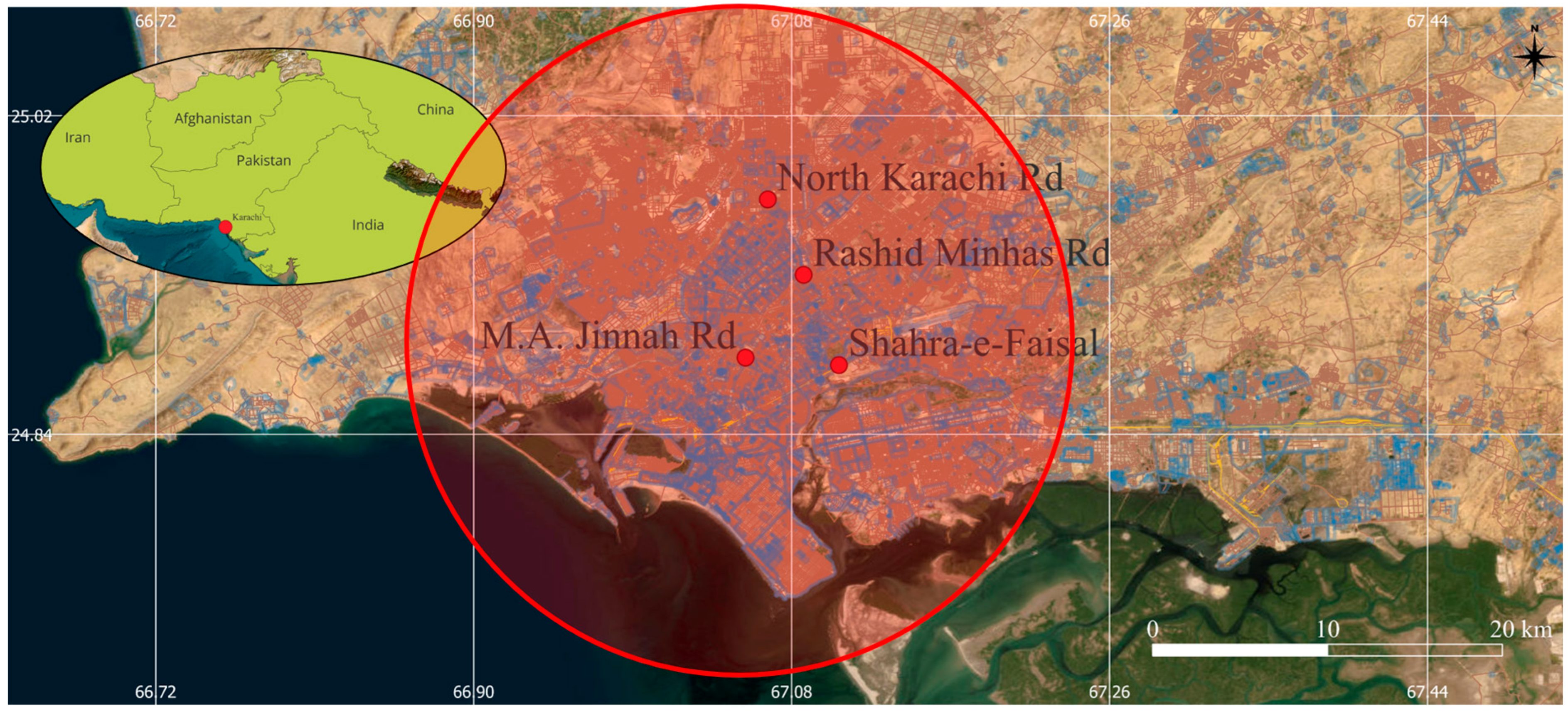
To analyze the relationship between PM levels and fluctuations in traffic volume and density, four major arterial roads in Karachi were selected based on their varying traffic patterns throughout the day, ensuring a diverse and representative dataset. Shahrah E Faisal Road, spanning 18 km (11 mi), is one of the most congested routes in Karachi, frequently experiencing traffic jams, and is located 13.7 km (8.5 mi) from central Karachi. New M.A. Jinnah Road, situated near the mausoleum of Pakistan’s founder, Muhammad Ali Jinnah, serves as a primary arterial route for traffic heading toward downtown Karachi and is located 11.8 km (7.3 mi) from the city center. North Karachi Road, one of the city’s oldest roads, witnesses high traffic density during peak hours, leading to frequent congestion and is situated 3.6 km (2 mi) from central Karachi. Rashid Minhas Road, another major and heavily trafficked arterial, stretches 11 km (6.8 mi) in length and is located 5.9 km (3.6 mi) from central Karachi.

3.2. Data Collection

The primary objective of the data collection was to obtain comprehensive information on traffic volume, traffic counts, meteorological parameters, and particulate matter (PM) concentrations for the specified arterial roads. The geographic coordinates of the monitored arterial sections are presented in Table 1 (see Figure 1).

Table 1. Coordinates of the Selected Arterials.

Arterials	GPS Coordinates
	Latitude	Longitude
Shahrah E Faisal Road	24°52′44.8″ N	67°06′24.5″ E
New M.A. Jinnah Road	24°52′59.8″ N	67°03′13.9″ E
North Karachi Road	24°58′21.7″ N	67°03′59.4″ E
Rashid Minhas Road	24°55′48.3″ N	67°05′12.3″ E

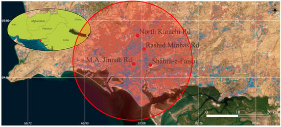
Figure 1. Locations of the monitored arterials.

Data collection was conducted over 16-h periods (06:00 to 22:00) on weekdays during April and May 2022. Each of the studied arterials was sampled for a single day to test the feasibility of combining statistical and Machine Learning models for urban PM prediction. The dataset does not capture day-to-day variability, weekend–weekday differences, seasonal patterns, or long-term trends. Therefore, the measurements should be interpreted as snapshots of typical weekday conditions rather than as representative of annual or seasonal air quality in Karachi.

All data—including particulate matter (PM), meteorological parameters, and traffic counts—were collected simultaneously at 10-min intervals to ensure consistency and minimize temporal variability. This resulted in a total of 98 readings per site.

Particulate matter concentrations were measured using a laser-based PM monitoring device (HOLDPEAK HP-5800M, Zhuhai JiDa Huapu Instrument Co., Ltd., Zhuhai, China), which operates on the laser scattering principle. The instrument provides high-resolution air quality measurements for PM₁, PM_2.5 and PM₁₀. It features a detection range of 0–999.9 μg/m³ for PM_2.5 and 0–1999.9 μg/m³ for PM₁₀, with a measurement resolution of 0.1 μg/m³. Temperature (°C), wind speed (m/s), and humidity (%) were collected using a Mastech Multi-Function Environment Tester MS6300 (MASTECH, Shenzhen, China). Both the PM monitor and the meteorological tester were positioned on the roadway median.

Vehicle counts were obtained manually from video recordings. A single mobile phone camera, mounted on a tripod on pedestrian bridges or overpasses, was oriented toward incoming traffic to ensure a clear view. The number of vehicles passing in each 10-min interval was recorded and classified into six categories: cars, bikes, rickshaws, pickups, buses, and trucks.

The Passenger Car Equivalent (PCE) is a unit used to represent the impact of a large vehicle on a road by expressing it as the number of equivalent passenger vehicles. PCE factors, as presented in Table 2 [26], are used to convert heavy vehicle counts into their equivalent number of passenger cars. Both actual traffic counts and PCE volumes are crucial in traffic analysis, each serving a distinct purpose. While actual traffic counts provide direct data on the number of vehicles on a road, PCE volumes assess the impact of different vehicle types on traffic flow and road capacity. Examining both metrics allows for a more comprehensive understanding of traffic volume, congestion, and overall road usage dynamics.

Table 2. Vehicles Types and Respective PCE Factors.

Vehicle Type	PCE Factor
Cars	1.00
Motorcycles	0.25
Rickshaws	0.50
Pickups	1.50
Busses	2.50
Trucks	3.00

The graphs present the total traffic volume over 16 h and the average hourly traffic volume per lane, comparing actual vehicle counts and Passenger Car Equivalent (PCE) counts (Figure 2) across four major roads in Karachi.

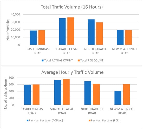
Figure 2. Total and Average Hourly Traffic Volumes.

In the Total Traffic Volume graph, Shahrah-e-Faisal Road has the highest traffic volume, with both actual counts and PCE counts close to 35,000 vehicles. North Karachi Road follows, though its PCE count is slightly lower than its actual count, indicating fewer heavy vehicles. Rashid Minhas Road shows nearly identical actual and PCE counts, suggesting a balanced mix of vehicle types. New M.A. Jinnah Road has the lowest traffic volume, with actual and PCE counts closely aligned around 17,000 vehicles.

In the Average Hourly Traffic Volume graph, Shahrah-e-Faisal Road again exhibits the highest traffic flow, with both actual and PCE values nearing 750 vehicles per hour per lane. North Karachi Road follows with slightly lower volumes. Rashid Minhas Road has moderate traffic, with actual and PCE counts closely matching at around 600 vehicles per hour. New M.A. Jinnah Road, despite having the lowest total traffic volume, shows a significant increase in PCE compared to actual counts, indicating a higher proportion of heavy vehicles that contribute more to road occupancy and emissions.

Table 3 presents the traffic composition across four major arterials studied, highlighting the variability in vehicle types. Rashid Minhas Road has the highest percentage of rickshaws (28%) and pickups (21%), indicating a significant presence of intermediate and light commercial vehicles. Shahrah-e-Faisal Road is dominated by cars (35%) and bikes (40%), with minimal representation of buses and trucks (1% each), reflecting its use primarily for personal and two-wheeler transport. North Karachi Road shows a balanced composition, with a notable share of bikes (36%) and cars (26%), along with a moderate presence of pickups (17%). New M.A. Jinnah Road exhibits a more diverse mix, with cars (24%), bikes (29%), and rickshaws (20%) forming the bulk of the traffic. When combined, all arterials show that bikes (32%) and cars (25%) are the predominant vehicle types, while trucks (4%) and buses (5%) have the lowest proportions.

Table 3. Traffic Composition.

	Cars	Bikes	Rikshaws	Pickups	Buses	Trucks
Rashid Minhas Road	14%	24%	28%	21%	7%	6%
Shahrah E Faisal Road	35%	40%	24%	0%	1%	1%
North Karachi Road	26%	36%	14%	17%	4%	4%
New M.A. Jinnah Road	24%	29%	20%	14%	7%	7%
All Combined	25%	32%	21%	13%	5%	4%

Descriptive statistical analysis was performed on the dataset, including the mean, standard deviation, minimum, maximum, and percentiles for each variable. The descriptive statistics are given in Table 4.

Table 4. Descriptive statistics of the data.

	Temperature (°C)	Wind (m/s)	Humidity (%)	PM1	PM2.5	PM10	Hourly Equivalent Traffic Volume in PCE (Veh/h)
count	388	388	388	388	388	388	388
mean	29.5	1.4	54.8	68.3	79.0	85.2	1630
std	6.4	0.9	14.7	22.5	26.4	27.5	548
min	14.4	0.2	19.4	20.0	19.0	19.0	393
25%	25.1	0.7	43.3	50.0	60.0	70.0	1221
50%	30.5	1.0	5.3	70.5	79.0	81.0	1448
75%	34.7	1.9	67.1	88.0	95.0	99.0	1996
max	40.5	4.1	86.1	166.0	160.0	190.0	3107

The data was used to analyze the impact of these independent variables on PM levels and to determine whether wind speed significantly reduces PM concentrations beyond specific thresholds.

The WHO Air Quality Guidelines’ recommended levels and interim targets for common air pollutants were revised in 2021, with more stringent limits compared to the previous 2005 guidelines. These updated guidelines are based on the latest scientific evidence regarding the health effects of air pollution. A comparison between the 2005 and 2021 air quality guidelines can be seen in Table 5 [27].

Table 5. WHO Air Quality Guidelines.

Pollutant	Averaging Time	2005 AQGs	2021 AQGs
PM2.5 μg/m3	Annual	10	5
	24-Hours	25	15
PM10 μg/m3	Annual	20	15
	24-Hours	50	45

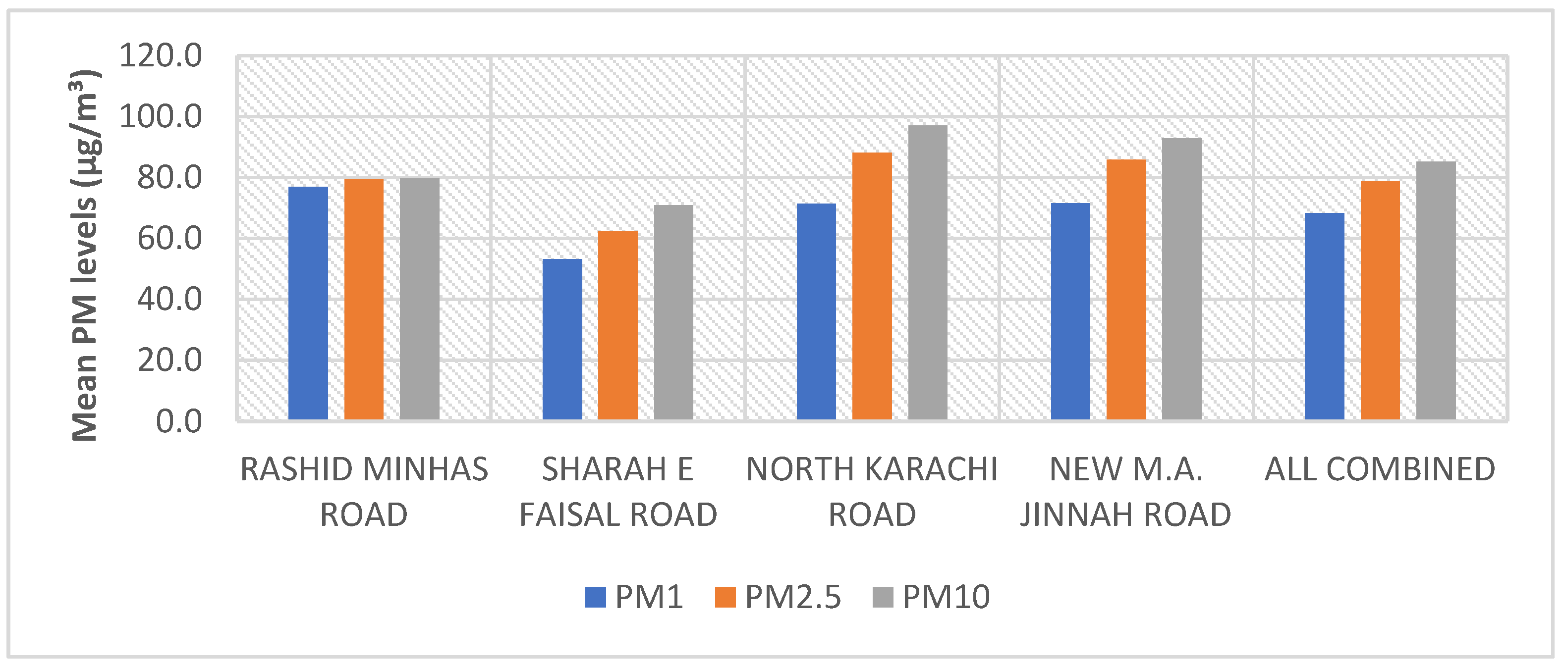
Figure 3 illustrates the concentrations of PM_2.5 and PM₁₀ across four major arterial roads in Karachi, benchmarked against the WHO Air Quality Guidelines (AQGs) from 2005 and 2021.

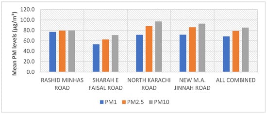
Figure 3. Mean PM Levels.

For the PM_2.5, all recorded values exceed both the 2005 AQG limit of 25 µg/m³ and the more stringent 2021 limit of 15 µg/m³. North Karachi Road exhibits the highest PM_2.5 concentration, nearing 90 µg/m³, followed closely by New M.A. Jinnah Road. Although Shahrah-e-Faisal Road shows the lowest PM_2.5 levels, they remain significantly above the permissible thresholds. The combined average PM_2.5 concentration across all sites is approximately four times the 2021 AQG, indicating critical levels of particulate pollution.

The PM₁₀ figures similarly reveal that all measured concentrations surpass the 2005 AQG limit of 50 µg/m³ and the 2021 limit of 45 µg/m³. North Karachi Road again registers the highest PM₁₀ levels, exceeding 90 µg/m³, while Shahrah-e-Faisal Road records the lowest levels, albeit still above recommended limits. The combined PM₁₀ levels reflect a substantial exceedance of WHO standards (Figure 4).

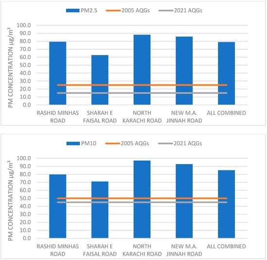
Figure 4. Measured PM_2.5 and PM₁₀ Comparison with AQGs Limit Values.

These findings underscore severe air quality challenges in Karachi, with PM levels well above international health guidelines. Elevated concentrations, particularly along North Karachi Road and New M.A. Jinnah Road, suggest substantial contributions from vehicular emissions and insufficient pollution control measures, posing significant public health risks.

4. Methodology and Results

4.1. Ordinary Least Squares (OLS) Regression Analysis

Ordinary Least Squares (OLS) regression Analysis has been widely applied by various researchers in the study of air pollution [28,29,30,31,32], whether to study the relationship between the pollutants and the environments or to acquire the estimates for the pollutants.

OLS regression was employed for analyzing the collected data due to its straightforward and effective approach. This statistical technique is used to assess the relationship between a dependent variable and multiple predictor variables. The results of the OLS regression are presented as coefficients, which serve as estimates of the impact each independent variable has on the dependent variable. By utilizing OLS regression, the analysis quantifies the extent to which each predictor variable contributes to variations in the dependent variable, providing a clearer understanding of the underlying relationships within the dataset [33].

$$Y=b_0 + B_1{X}_1+b_2{X}_2+\dots +b_n{x}_n+\epsilon$$

where

• y = The predicted value of the dependent variable.
• b₀ = The y-intercept, representing the value of y when all independent variables are zero.
• b₁ × 1 = The regression coefficient (B₁) of the first independent variable (X₁), indicating the impact of X₁ on the predicted y value.
• b_nX_n = The regression coefficient of the last independent variable, showing its influence on y.
• ε = The model error, representing the unexplained variation in the predicted y value.

In this study, particulate matter (PM) serves as the dependent variable, while temperature, wind, and PCE count act as the independent variables. The B values represent the regression coefficients for temperature, wind, and PCE count, indicating their respective influences on PM levels. Predictor variables were not standardized prior to analysis. This approach was chosen to maintain the physical interpretability of the OLS regression coefficients (representing the change in PM concentration per unit change in the predictor) and because the primary comparison model, Random Forest, is invariant to monotonic feature scaling.

All pairwise correlations fall well below established thresholds associated with multicollinearity (|r| ≥ 0.7), with the highest coefficient observed between wind speed and traffic volume (r = 0.24), reflecting only a weak association (Table 6). Similarly, temperature and humidity demonstrated only a modest negative correlation (r = −0.20). Collectively, these findings confirm that the degree of shared variance among predictors is minimal and does not compromise the robustness or interpretability of the OLS regression estimates.

Table 6. Pairwise Pearson correlations among the OLS predictors.

Predictor	Temperature	Humidity	Wind	Traffic Volume
Temperature (°C)	1.00	−0.20	0.01	−0.18
Humidity (%)	−0.20	1.00	0.03	−0.13
Wind (m/s)	0.01	0.03	1.00	0.24
Hourly Equivalent Traffic Volume	−0.18	−0.13	0.24	1.00

Certain statistical measures, including the coefficient of determination (R²) and the Root Mean Square Error (RMSE), are employed to assess the performance of the model. The corresponding formulas are presented below:

R² represents the overall proportion of variance in the dependent variable that is explained by the combination of all predictor variables [33].

$$R^2=1-{\displaystyle \frac{\sum ({yi-\widehat{yi})}^2}{\sum ({yi-\overline{yi})}^2}}$$

where

• $\mathrm{y}\mathrm{i}=\mathrm{o}\mathrm{b}\mathrm{s}\mathrm{e}\mathrm{r}\mathrm{v}\mathrm{e}\mathrm{d} \mathrm{v}\mathrm{a}\mathrm{l}\mathrm{u}\mathrm{e}\mathrm{s}$;
• $\widehat{\mathrm{y}\mathrm{i}}=\mathrm{p}\mathrm{r}\mathrm{e}\mathrm{d}\mathrm{i}\mathrm{c}\mathrm{t}\mathrm{e}\mathrm{d} \mathrm{v}\mathrm{a}\mathrm{l}\mathrm{u}\mathrm{e}\mathrm{s}$;
• $\overline{\mathrm{y}\mathrm{i}}=\mathrm{m}\mathrm{e}\mathrm{a}\mathrm{n} \mathrm{o}\mathrm{f} \mathrm{o}\mathrm{b}\mathrm{s}\mathrm{e}\mathrm{r}\mathrm{v}\mathrm{e}\mathrm{d} \mathrm{v}\mathrm{a}\mathrm{l}\mathrm{u}\mathrm{e}\mathrm{s}$.

The Root Mean Squared Error (RMSE) represents the standard deviation of residuals.

$$RMSE=\sqrt{{\displaystyle \frac{1}{n}}\sum _{i=1}^n({yi-\widehat{yi})}^2}$$

where

• $\mathrm{y}\mathrm{i}=\mathrm{o}\mathrm{b}\mathrm{s}\mathrm{e}\mathrm{r}\mathrm{v}\mathrm{e}\mathrm{d} \mathrm{v}\mathrm{a}\mathrm{l}\mathrm{u}\mathrm{e}\mathrm{s}$;
• $\widehat{\mathrm{y}\mathrm{i}}=\mathrm{p}\mathrm{r}\mathrm{e}\mathrm{d}\mathrm{i}\mathrm{c}\mathrm{t}\mathrm{e}\mathrm{d} \mathrm{v}\mathrm{a}\mathrm{l}\mathrm{u}\mathrm{e}\mathrm{s}$;
• $\overline{\mathrm{y}\mathrm{i}}=\mathrm{n}\mathrm{u}\mathrm{m}\mathrm{b}\mathrm{e}\mathrm{r} \mathrm{o}\mathrm{f} \mathrm{o}\mathrm{b}\mathrm{s}\mathrm{e}\mathrm{r}\mathrm{v}\mathrm{a}\mathrm{t}\mathrm{i}\mathrm{o}\mathrm{n}\mathrm{s}$;

A series of multiple linear regressions were performed, where PM₁, PM_2.5, and PM₁₀ were the dependent variables, and temperature, wind speed, humidity, and traffic volume were the independent variables. It is important to note that these models were run without an intercept. While an intercept typically represents background concentrations in source apportionment, its interpretation becomes ambiguous when predictors like Temperature and Humidity are included, as ‘zero’ values for these parameters (0 °C, 0%) are physically impossible in the study context (the minimum observed temperature was 14.4 °C). A calculated intercept would, therefore, represent a mathematical extrapolation to non-existent atmospheric conditions rather than a tangible background level. By suppressing the intercept, we focus the regression strictly on the covariance between the observed predictors and PM levels. This approach was deemed appropriate given that the OLS models serve primarily as a baseline to demonstrate the limitations of linear assumptions compared to the non-linear Random Forest model.

The estimated weights of the independent variables are calculated, and the t statistics are included in parenthesis in Equations (1)–(3).

PM₁ = 0.0040 × Traffic Volume (1.90) + 1.4232 × Temperature (10.58) − 5.0286 × Wind Speed (−3.46) + 0.4621 × Humidity (6.82)

(1)

PM_2.5 = 0.0069 × Traffic Volume (2.77) + 1.1668 × Temperature (7.28) − 3.1355 × Wind Speed (−1.81) + 0.6525 × Humidity (8.08)

(2)

PM₁₀ = 0.0090 × Traffic Volume (3.45) + 1.0198 × Temperature (6.08) − 3.1143 × Wind Speed (−1.72) + 0.7797 × Humidity (9.23)

(3)

The results indicate that temperature and humidity have a strong influence on PM levels, showing high significance across all models. Wind speed is significant for PM₁ and moderately significant for PM_2.5 and PM₁₀. Traffic volume is statistically significant for PM_2.5 and PM₁₀, but its effect on PM₁ is weaker.

The t-statistics and p-values provide critical insights into the significance and strength of these relationships. Higher t-values denote stronger relationships, while negative t-values reflect inverse correlations, emphasizing the importance of considering both magnitude and significance in environmental modeling.

In the PM₁ model, temperature (t = 10.58, p = 0.000) and humidity (t = 6.82, p = 0.000) exhibit highly significant positive effects, while wind speed (t = −3.46, p = 0.001) significantly reduces PM₁ concentrations. Traffic volume (t = 1.90, p = 0.058) shows a weaker association due to its marginal p-value.

In the PM_2.5 model, temperature (t = 7.28, p = 0.000), humidity (t = 8.08, p = 0.000), and traffic volume (t = 2.77, p = 0.006) are significant contributors, while wind speed (t = −1.81, p = 0.071) suggests a potential inverse relationship despite not meeting the 0.05 significance level.

For PM₁₀, temperature (t = 6.08, p = 0.000), humidity (t = 9.23, p = 0.000), and traffic volume (t = 3.45, p = 0.001) are significant predictors, whereas wind speed (t = −1.72, p = 0.087) indicates a possible negative effect. Lower p-values (< 0.05) provide strong evidence against the null hypothesis, confirming the significance of these predictors on PM levels.

4.2. Random Forest Regression Analysis

Random Forest is a supervised machine learning algorithm used for classification and regression. It builds multiple decision trees from random subsets of data and features, then combines their results to improve accuracy and reduce overfitting. Based on the bagging (Bootstrap Aggregating) technique, it trains each tree independently on bootstrapped samples. The final prediction is an average (for regression) or majority vote (for classification) of all trees. The flow diagram of the Random Forest algorithm is provided in Figure 5. Random Forest does not assume linear relationships, making it effective for complex, non-linear datasets. Its key steps include bootstrap sampling, random feature selection, tree construction, and aggregation of predictions to produce a robust ensemble model. The key Random Forest parameters employed in this study are presented in Table 7.

Figure 5. Flow Diagram of Random Forest.

Table 7. Key Random Forest Parameters.

Parameter	Description	Plausible Range	Value Used
n_estimators	Number of decision trees in the Random Forest model, improving accuracy with more trees	50 to 1000 (increments of 50 or 100)	100
max_depth	Maximum depth of each tree, controlling model complexity and preventing overfitting	5 to 50, or None (for unlimited depth)	None (unlimited depth)
max_features	Number of features considered for the best split, such as sqrt, log2, or a fraction	sqrt, log2, or a float between 0.1 and 1.0	1.0 (all features considered)
min_samples_split	Minimum samples required to split an internal node, influencing model complexity	2 to 20	2
min_samples_leaf	Minimum samples required at a leaf node, controlling overfitting	1 to 20	1
bootstrap	Indicates if bootstrap sampling is used to train each tree on a random data subset	True or False	TRUE
oob_score	Uses out-of-bag samples to estimate R2 without a separate validation set	True or False	FALSE
random_state	Sets a seed for reproducibility, ensuring consistent results across model runs	Any integer value	42

Random Forest has proven highly effective in environmental and emissions modeling, particularly for air quality prediction, pollutant dispersion, and traffic emission estimation. It surpasses traditional linear models by capturing complex, non-linear interactions among environmental variables. The model’s performance depends on several key parameters, including the number and depth of trees, the number of features per split, the minimum number of samples for nodes, bootstrap sampling, out-of-bag validation, and random states, all optimized to balance complexity, accuracy, and computational efficiency.

Its application is demonstrated in several studies. Random Forest has been applied to estimate high-resolution PM_2.5 levels in the North China Plain with remarkable accuracy, even for historical data [34]. Similarly, it has been utilized to predict daily PM_2.5 concentrations in urban areas at a 1 × 1 km resolution, outperforming traditional approaches [35]. In a related study, Random Forest was compared with land use regression models for elemental PM components and found superior accuracy in capturing pollutant–land use relationships [36]. These studies highlight the algorithm’s robustness and adaptability in air quality modeling.

Recent research has also employed other advanced machine learning methods—particularly XGBoost, Artificial Neural Networks (ANNs), and Long Short-Term Memory (LSTM) networks—to improve air-quality forecasting. A study from Malaysia in 2023 demonstrated that multi-layer feedforward neural networks can achieve highly accurate PM_2.5 predictions, with the Levenberg–Marquardt–trained FBNN model attaining an R² of 0.98 and the lowest associated error metrics among the evaluated algorithms [37]. A two-stage feature engineering framework employed in a study in UK, combining correlation-inspired feature construction with Variational Mode Decomposition, substantially enhanced the performance of an LSTM-based forecasting model for multiple pollutants (NO₂, O₃, SO₂, PM_2.5, and PM₁₀), yielding a 13% improvement in R² and the lowest RMSE and MAE values among the tested configurations [38].

Further demonstrating the power of these techniques, a spatially local XGBoost (SL-XGB) framework integrating high-resolution SARA AOD with locally optimized machine-learning models achieved markedly improved urban-scale PM_2.5 estimation in Beijing (R² ≈ 0.88) relative to standard XGBoost and GWR, demonstrating enhanced capacity to capture both non-linear relationships and spatial heterogeneity in areas with sparse monitoring coverage [39]. A recent study from the Middle East demonstrated that Multilayer Perceptron (MLP) neural networks outperform multiple linear regression in predicting seasonal and intra-annual PM₁₀ and PM_2.5 concentrations using meteorological variables and AOD, achieving correlations up to 0.81 and highlighting the strong seasonal dependence and dominant influence of relative humidity on particulate-matter levels [40]. A recent study for Shanghai developed an enhanced XGBoost-based forecasting framework that integrates empirical mode decomposition, model fusion, and spatial optimization techniques, achieving a 17% improvement in goodness of fit and a 28% reduction in RMSE for PM_2.5 prediction, while also revealing strong seasonal patterns and clear urban–rural gradients in particulate-matter concentrations [41].

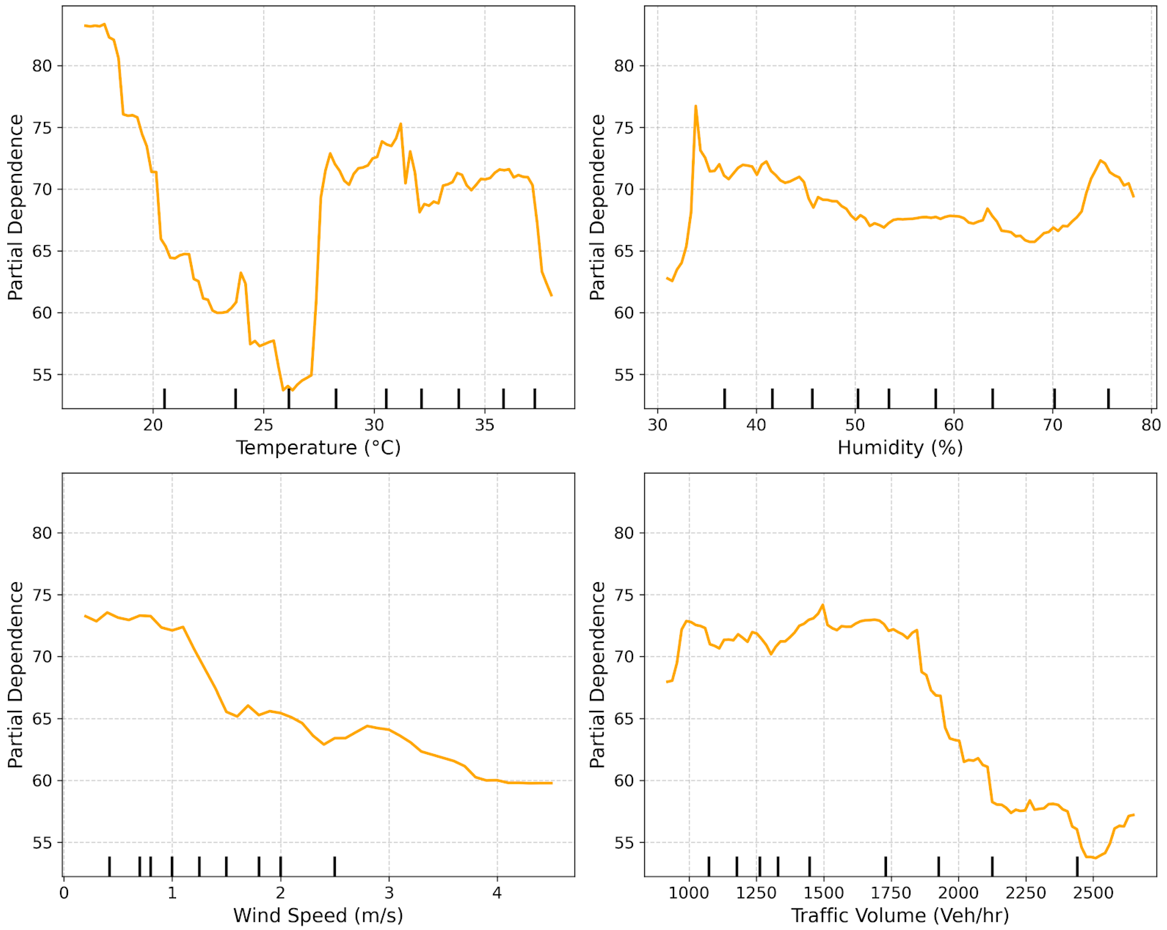
The partial dependence plots derived from Random Forest meteorological-normalization models provide interpretable insights into the physical and chemical drivers of PM₁₀ variability, revealing distinct regimes associated with poor dispersion and secondary aerosol formation that help explain long-term particulate-matter trends in Switzerland [42]. Furthermore, partial dependence analyses were conducted to observe the possibility of non-linear relationships between the predictor variables and particulate matter concentrations. Figure 6 presents the PDPs for PM₁ across the meteorological and traffic variables, and similar response patterns were observed for PM_2.5 and PM₁₀.

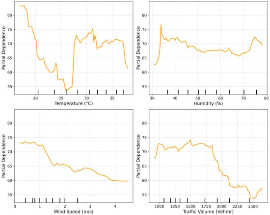
Figure 6. PDP for PM₁ and meteorological and traffic variables.

Temperature exhibited a distinctly non-linear pattern across all PM fractions (PM₁, PM_2.5, and PM₁₀), with concentrations decreasing around 22–25 °C and subsequently stabilizing or increasing at higher temperatures, likely reflecting the combined influence of atmospheric mixing and evaporation. Humidity showed a characteristic U-shaped response, where low humidity levels were associated with reduced PM concentrations due to enhanced atmospheric dispersion, while very high humidity corresponded to elevated PM levels, consistent with hygroscopic particle growth. Wind speed demonstrated a consistently negative non-linear effect on all PM metrics, indicating that higher wind speeds promote pollutant dilution and dispersion. Traffic volume displayed a saturating non-linear pattern.

PM levels increased with traffic load up to approximately 2000 veh/hr, beyond which concentrations plateaued or slightly decreased, suggesting that emissions dominate under moderate traffic, whereas intensified turbulence under very high traffic density enhances dispersion. These findings underscore the ability of the Random Forest model to capture complex, non-linear atmospheric and emission-driven dynamics that are not adequately represented by linear regression approaches.

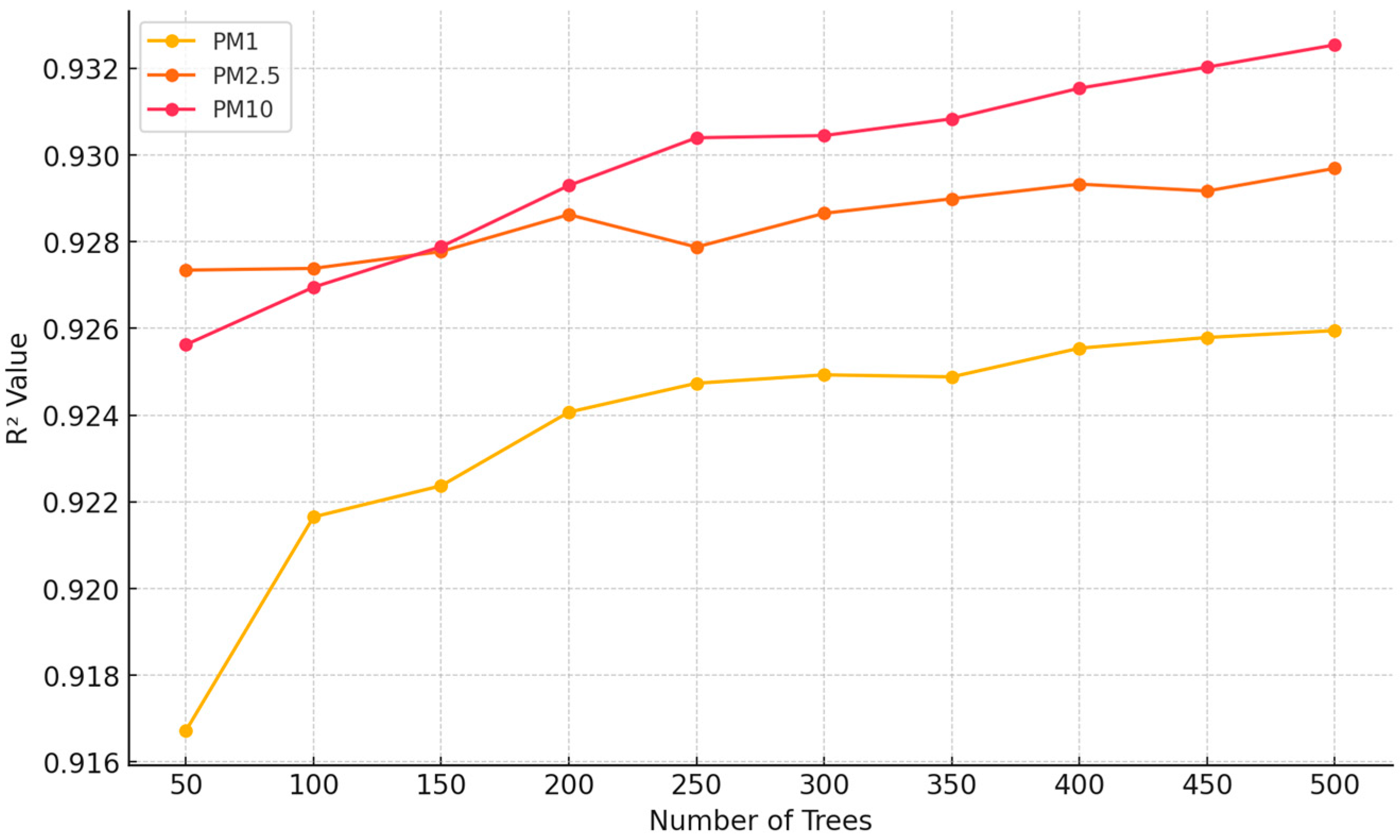
Figure 7 shows the R² values for Random Forest models predicting PM₁, PM_2.5, and PM₁₀ as the number of trees increases from 50 to 500.

Figure 7. Number of Trees vs. R² Values.

PM₁₀ exhibits the highest R² values across all tree counts, showing a consistent upward trend and reaching its peak (~0.93) at 500 trees. PM_2.5 starts at a relatively high R² (~0.93) with minor fluctuations but generally improves as more trees are added, also peaking at around 0.93. PM₁, which starts with the lowest R² (~0.917) at 50 trees, displays a steady improvement, reaching approximately 0.926 at 500 trees. The most significant improvement for PM₁ was observed between 50 and 150 trees before the values stabilized.

Overall, increasing the number of trees enhances the model’s R² values for all PM metrics, though the improvements diminish beyond 200–300 trees. Notably, PM₁₀ predictions benefit the most from a higher number of trees, while PM₁ shows the most noticeable improvement with increasing tree counts. The results suggest that using around 300–400 trees strikes a balance between computational cost and model accuracy, as the R² gains become marginal beyond this range.

It is important to note that the R² values shown in Figure 7 were calculated on the training dataset to illustrate model performance as the number of trees increased.

Using a manually configured high-capacity Random Forest regressor (800 trees, unrestricted depth, and a square-root feature selection strategy), the model achieved high coefficients of determination across all pollutants (R² = 0.93–0.94) when evaluated on the training dataset. These results indicate that the model can explain over 92% of the variance in PM₁, PM_2.5, and PM₁₀ concentrations. The low RMSE values (6–7 µg/m³) further reflect a strong in-sample fit. This high-capacity configuration was chosen deliberately to approximate previously observed high training R² values (~0.93), allowing the model to fully exploit nonlinearities in the data without any hyperparameter tuning for the cross-validation stage.

However, these performance values are inherently optimistic, as the model was evaluated on the same data used for training. The hyperparameter choices—particularly the large number of trees and absence of depth constraints—enabled the model to effectively memorize the training set. Therefore, these R² values represent the upper bound of model performance rather than a realistic measure of predictive accuracy on unseen data.

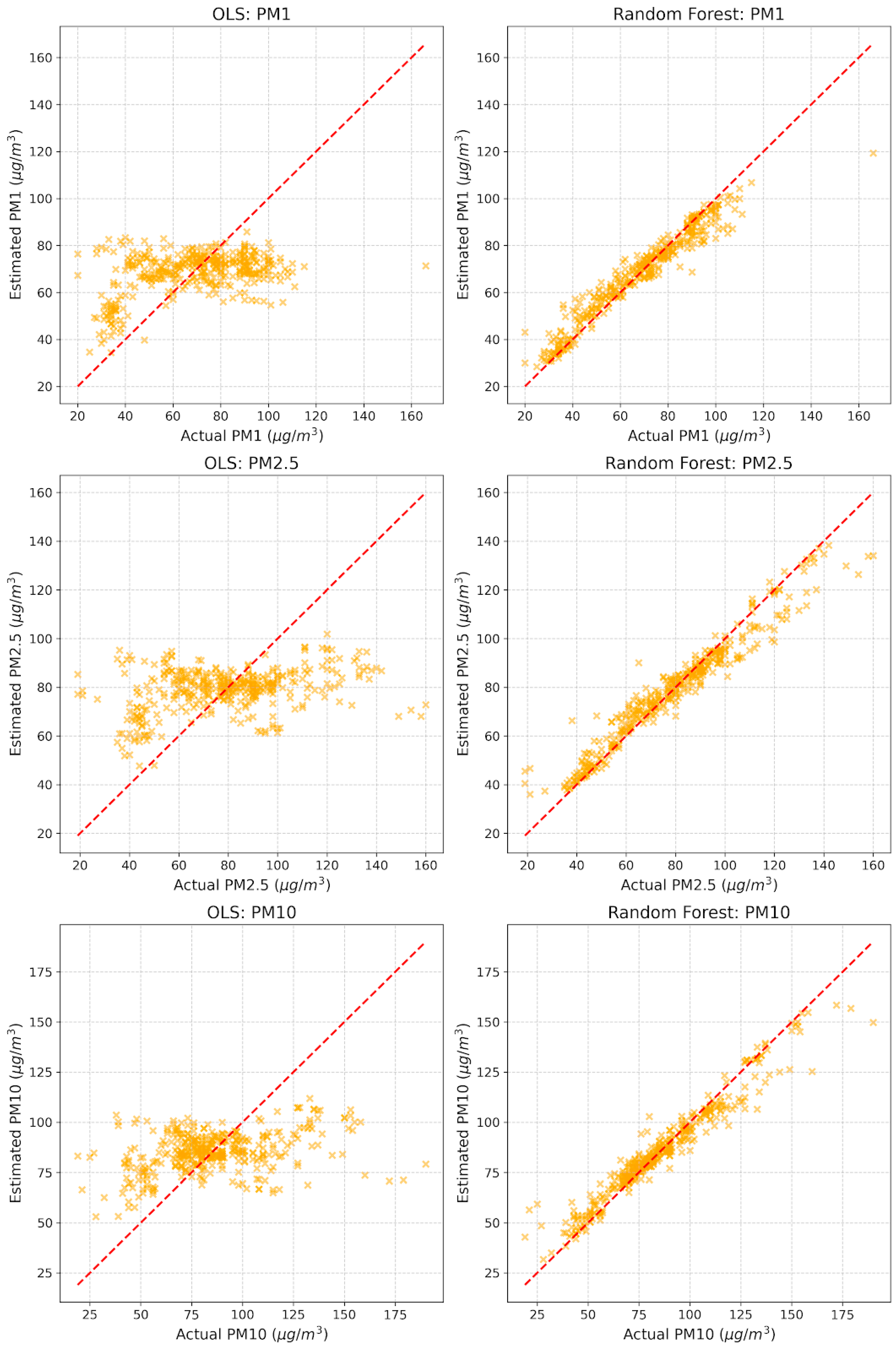
Overall, the results show that Random Forest regression provided higher R² values compared to OLS, indicating better performance in capturing the variability in PM levels. This method is suitable when non-linear interactions and complex dependencies exist in the dataset. The RMSE values confirm that the Random Forest model has significantly lower errors compared to OLS, further demonstrating its superior accuracy and performance. The analysis also includes side-by-side plots (Figure 8) comparing estimated PM levels from OLS and Random Forest models to actual PM levels for each PM type, clearly demonstrating the improved accuracy of Random Forest predictions over OLS (see Table 8).

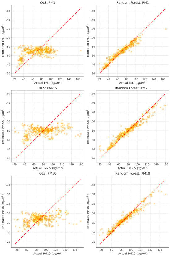
Figure 8. Estimated vs. Actual PM Levels for OLS and Random Forest.

Table 8. Comparison of OLS and RF results.

PM Metric	OLS R2	Random Forest R2	OLS RMSE	Random Forest RMSE
PM1	0.1614	0.9284	20.61	6.02
PM2.5	0.1119	0.9306	24.84	6.94
PM10	0.1284	0.9347	25.68	7.03

To obtain an unbiased estimate of the model’s out-of-sample predictive performance, a 5-fold cross-validation strategy was employed for each particulate matter (PM) metric. The entire dataset was randomly partitioned into five mutually exclusive and approximately equal-sized folds using a randomized K-fold procedure (KFold with five splits, shuffling enabled, and a fixed random seed for reproducibility).

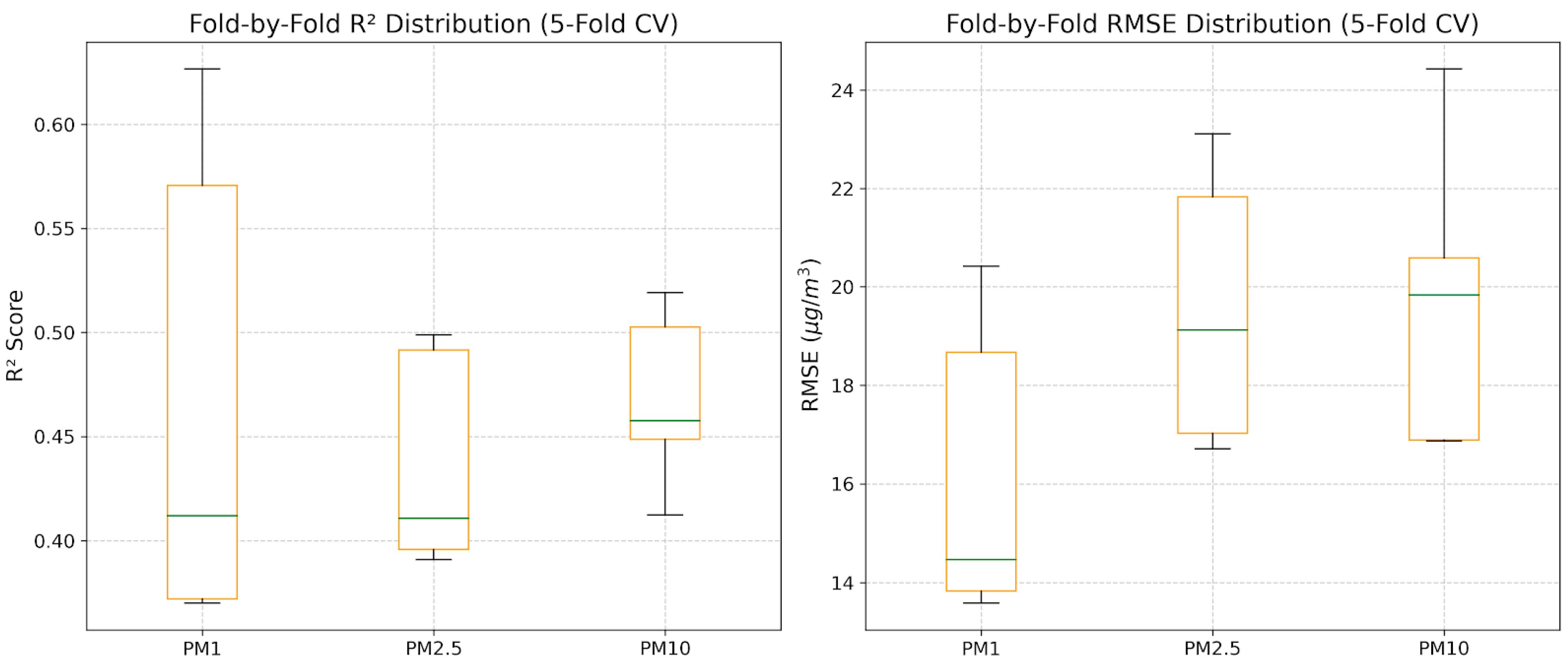
For each iteration, the model was trained on four folds (80% of the data) and evaluated on the remaining held-out fold (20%), ensuring no overlap between training and validation samples. Predictions were generated for each held-out fold, and the coefficient of determination (R²) and root mean square error (RMSE) were computed. This procedure was repeated five times so that each observation was used exactly once for validation. The resulting R² and RMSE values were aggregated across the folds, and both the mean values and fold-specific distributions were reported. This procedure yielded fold-wise R² and RMSE values, whose distributions were summarized using boxplots (Figure 9) to assess predictive stability and variance across folds. To obtain unbiased estimates of generalization performance, a 5-fold cross-validation procedure was later employed, as reported in Table 9.

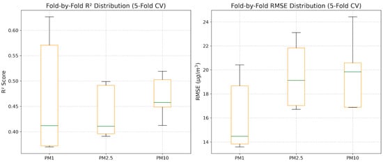
Figure 9. Distribution of model performance metrics across 5-Fold Cross-Validation.

Table 9. K-fold cross-validation strategy RF results.

PM Metric	CV RF R2	Random Forest R2	CV RF RMSE	Random Forest RMSE
PM1	0.47	0.93	16.44	6.02
PM2.5	0.45	0.93	19.51	6.94
PM10	0.51	0.94	19.33	7.03

This approach provides a more reliable evaluation than a single train–test split, as it mitigates optimistic bias associated with training-set evaluation and reduces variance arising from arbitrary data partitioning. Cross-validation is particularly appropriate for environmental datasets such as PM measurements, where the number of observations may be limited and temporal or meteorological fluctuations can affect model generalization. By applying the same high-capacity Random Forest configuration across multiple folds, the reported R² values reflect the model’s genuine ability to generalize to unseen subsets of the data distribution rather than its capacity to memorize the training data.

Table 9 presents the results of the Random Forest (RF) model under 5-fold cross-validation and 100% training evaluation, while Table 8 provides a comparative summary of the RF and Ordinary Least Squares (OLS) regression models. While hyperparameter tuning (e.g., limiting tree depth) could reduce this gap, we deliberately retained the high-capacity configuration to explicitly demonstrate the contrast between model fitting potential and true generalization power, thereby highlighting the necessity of cross-validation in environmental modeling.

Together, these results highlight both the superior in-sample fitting ability of RF compared to OLS and the discrepancy between training and cross-validated performance for the RF model.

In Table 8, the RF model achieves high R² values on the training data for all PM metrics (0.93 for PM₁, 0.93 for PM_2.5, and 0.94 for PM₁₀) with low RMSE values (6.02–7.03 µg/m³), indicating an excellent fit to the training dataset. However, the corresponding cross-validated R² values are substantially lower (0.47 for PM₁, 0.45 for PM_2.5, and 0.51 for PM₁₀), and the RMSE values increase to 16.44–19.51 µg/m³. This gap between training and cross-validation performance reflects the overfitting tendency of the high-capacity RF configuration: while the model is able to explain over 93% of the variance in the training data, its ability to generalize to unseen data is more modest, with R² values in the 0.45–0.51 range.

The implication for model generalizability is that the reported training metrics (R² > 0.9) represent an upper theoretical bound of explanatory power, effectively capturing local noise and specific traffic-meteorology interactions. In contrast, the cross-validated metrics (R² ≈ 0.5) serve as the realistic indicator of operational predictive performance on unseen data. Consequently, while the unconstrained Random Forest model proves superior to OLS in detecting non-linear signals, any practical deployment for future forecasting would strictly require the cross-validated performance estimates to be used as the baseline for accuracy expectations.

When compared with OLS results, the Random Forest clearly outperforms OLS in terms of in-sample predictive accuracy. OLS exhibits low R² values (0.16 for PM₁, 0.11 for PM_2.5, and 0.13 for PM₁₀) and high RMSE values (20.61–25.68 µg/m³), indicating a weak ability to model the complex relationships between meteorological, traffic, and pollutant concentration variables. In contrast, the RF model achieves R² values above 0.93 and reduces the RMSE by approximately 70% across all PM metrics. This performance gap illustrates the strength of nonlinear ensemble methods such as Random Forest in capturing complex, non-additive interactions that linear models cannot accommodate.

Interestingly, even under cross-validation, the RF model maintains substantially higher R² values than OLS, indicating that despite some overfitting, the RF model generalizes better than OLS to unseen subsets of the data. Among the three pollutants, PM₁₀ shows the highest cross-validated R² (0.51), suggesting a relatively more structured relationship between the predictors and PM₁₀ levels compared to PM₁ and PM_2.5.

Overall, these findings underscore two key points:

• Random Forest provides significant performance improvements over OLS, both in terms of R² and RMSE, demonstrating its capacity to model nonlinear environmental processes more effectively.
• Cross-validation is essential for obtaining realistic performance estimates, as training-set results alone can be misleadingly optimistic due to overfitting, particularly in flexible models like RF.

4.3. Wind Speed Threshold Analysis

The wind speed threshold was identified using piecewise regression, where the dataset was split at various wind speeds, and the best threshold was chosen based on the lowest mean squared error.

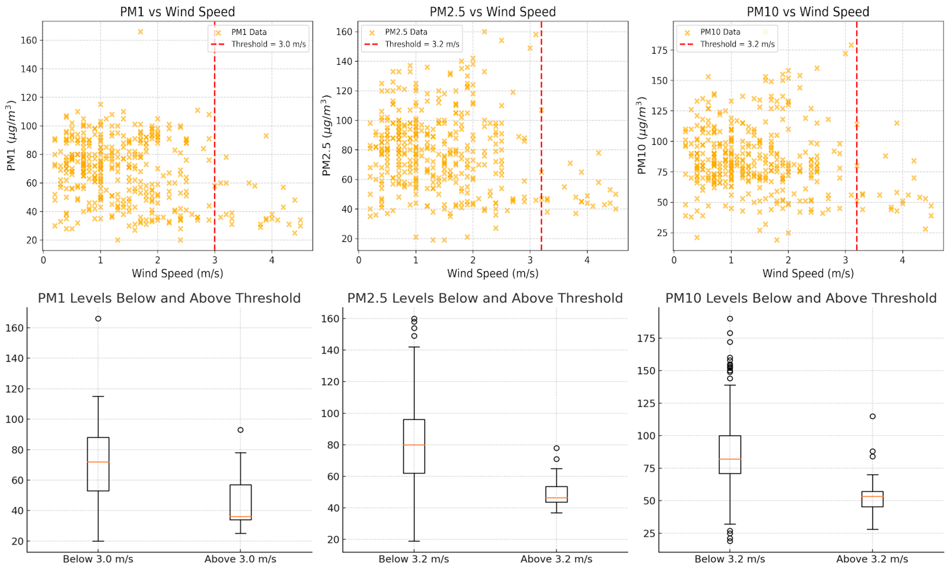
The relationship between wind speed and particulate matter (PM) concentrations was examined using a threshold analysis to identify critical wind speeds beyond which pollutant levels decrease markedly. This analysis was conducted in two stages: an initial exploratory visual inspection, followed by a formal piecewise linear regression to estimate the wind speed threshold in a data-driven manner. Scatter plots of PM₁, PM_2.5, and PM₁₀ concentrations against wind speed revealed a non-linear pattern, with concentrations remaining relatively stable at low wind speeds and decreasing sharply beyond approximately 3 m/s. To statistically determine this breakpoint, a piecewise linear regression model was fitted iteratively for each unique wind speed value T in the dataset. Specifically, the model assumes that the relationship between wind speed (x) and PM concentration (y) can be represented as two linear segments joined at the threshold T:

$$y_i= \left\{\begin{array}{l}{\mathrm{\beta }}_0+{\mathrm{\beta }}_1{\mathrm{x}}_i+ {\mathrm{\epsilon }}_i, \hspace{0.17em}{\mathrm{x}}_i\le T \\ {\mathrm{\beta }}_0+{\mathrm{\beta }}_{1}T+ {{\mathrm{\beta }}_2\left(x_i-T\right)+\mathrm{\epsilon }}_i, {\mathrm{x}}_i\ge T\end{array}\right.$$

where β₀ is the intercept, β₁ and β₂ are the slopes below and above the threshold, respectively, and ε_i is the error term for observation i. For computational implementation, wind speed was decomposed into two predictor variables (“xbelow” and “xabove”) defined as

$$x_{below,i}=\min (x_i,T),$$

$$x_{above,i}=\max ({0, x}_i-T),$$

allowing the model to be expressed in a linear form suitable for ordinary least squares estimation:

$$y_i={\mathrm{\beta }}_0+{\mathrm{\beta }}_1{x}_{below,i}+ {{\mathrm{\beta }}_2{x}_{above,i}+\mathrm{\epsilon }}_i$$

For each candidate threshold T, the model was fitted, and its performance was evaluated using the Mean Squared Error (MSE) criterion,

$$\mathrm{M}\mathrm{S}\mathrm{E}(\mathrm{T})={\displaystyle \frac{1}{n}}{\sum }_{i=n}^n{\left(\right(y_i-{\widehat{y}}_i \left(T\right))}^2,$$

where ${\widehat{y}}_i \left(T\right)$ denotes the predicted value under the model with threshold T. The optimal threshold was selected as the value of T that minimized the MSE, thus identifying the breakpoint that best explained the observed non-linear relationship. This procedure was repeated separately for PM₁, PM_2.5, and PM₁₀, yielding optimal thresholds of 3.0 m/s, 3.2 m/s, and 3.2 m/s, respectively (Table 10). These results indicate that when wind speeds exceed approximately 3 m/s, the concentrations of all measured PM fractions tend to decrease significantly, reflecting the physical process by which increased wind speeds enhance atmospheric mixing and pollutant dispersion. This threshold-based approach provides a robust statistical framework for identifying dispersion thresholds, which can inform both air quality modeling and regulatory strategies by delineating wind conditions under which pollutant accumulation is likely to occur.

Table 10. Wind Speed Thresholds for PMs.

PM Metric	Threshold Wind Speed (m/s)	t-Statistic	p-Value
PM1	3.0	7.45	2.67 × 10−8
PM2.5	3.2	11.04	1.45 × 10−12
PM10	3.2	6.49	1.24 × 10−6

The plots (Figure 10) show the PM levels against wind speed, with a red dashed line indicating the identified threshold wind speeds. PM₁ levels tend to stabilize and decrease when the wind speed surpasses 3.0 m/s. PM_2.5 levels show a noticeable drop after wind speeds exceed 3.2 m/s. Similarly, PM₁₀ levels significantly decrease once the wind speed goes beyond 3.2 m/s.

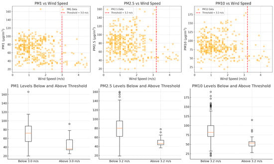
Figure 10. Wind Speed Thresholds for PMs.

When wind speeds exceed these threshold values, the concentration of particulate matter (PM₁, PM_2.5, or PM₁₀) tends to decrease significantly. This aligns with the physical expectation that higher wind speeds disperse pollutants more effectively. Below the thresholds, PM levels are more dispersed and higher, indicating that lower wind speeds are insufficient to disperse airborne particles effectively. Above these thresholds, PM levels consistently decrease, suggesting that wind speeds at or above ~3.0–3.2 m/s are effective in clearing particulate matter from the air.

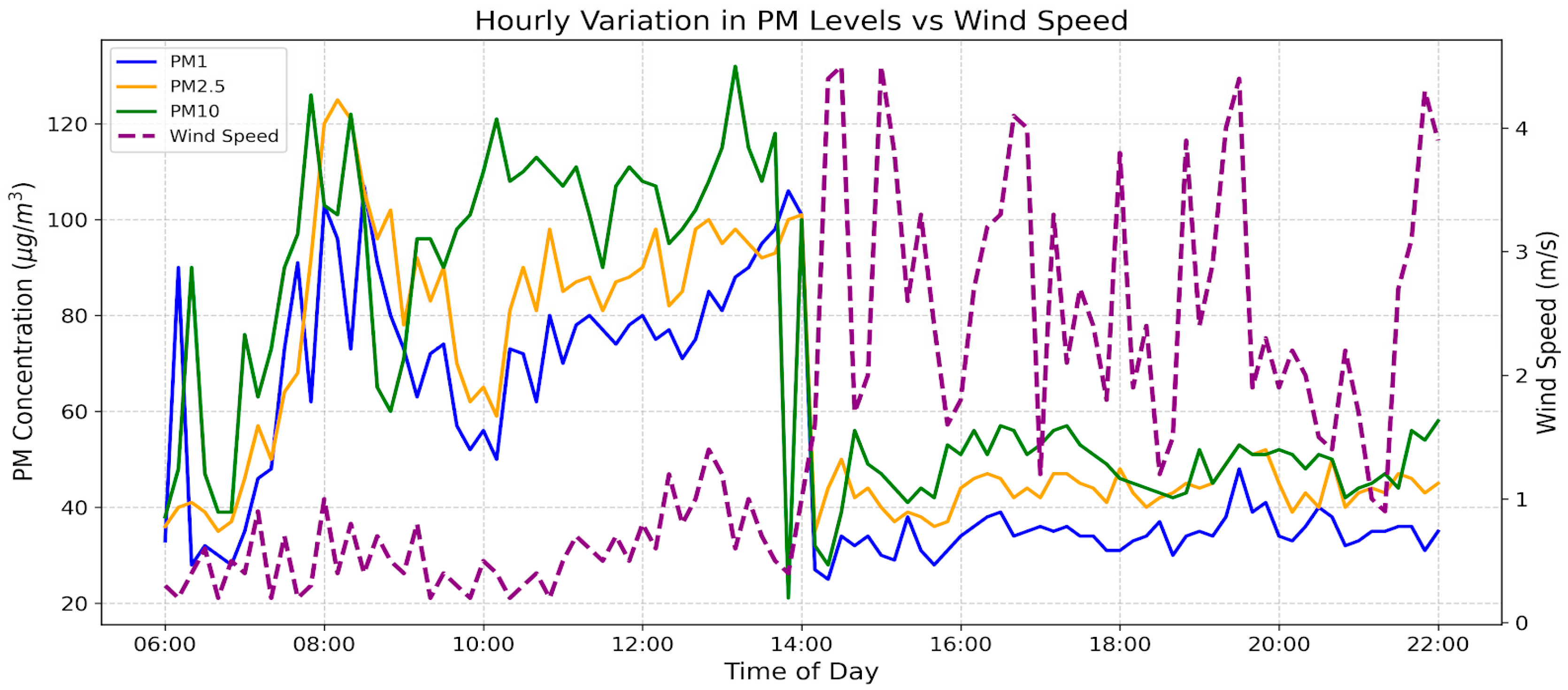
For validation purposes, the threshold analysis was visually inspected using the daily variation in PM levels and changes in wind speed. Figure 11. illustrates the hourly variation in PM₁, PM_2.5, and PM₁₀ levels alongside wind speed at Shahrah-e-Faisal, revealing an inverse relationship between wind speed and particulate matter concentrations. PM levels peak during the morning hours, particularly around 8:00–9:00 AM, coinciding with high traffic congestion and relatively low wind speeds. Throughout the day, PM levels fluctuate moderately but begin to decline significantly after 1:00 PM, when wind speed increases sharply. Wind speed peaks around 2:20 PM and continues to show periodic surges in the evening, contributing to a noticeable reduction in PM concentrations. This trend validates the threshold analysis, demonstrating that wind speeds above approximately 3–4.5 m/s effectively disperse airborne particulate matter, highlighting the crucial role of wind speed in mitigating air pollution at this arterial road.

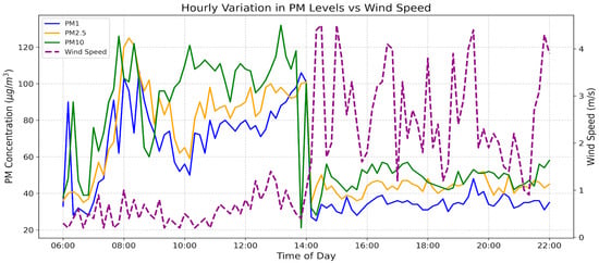
Figure 11. Hourly variation in particulate matter (PM) levels vs. wind speed.

In conclusion, these threshold values could serve as benchmarks for urban air quality management, indicating that maintaining wind speeds above these levels (through strategic city planning or monitoring) can significantly improve air quality.

5. Discussion

This study investigated the relationship between particulate matter (PM) concentrations and meteorological parameters—specifically temperature, humidity and wind—while also considering the impact of traffic volume.

The analysis identified temperature and humidity as key influences, with both variables showing high significance and a strong positive relationship with PM levels across all models, underscoring the critical role of meteorological factors in air quality. Wind speed also played an important role, exhibiting a significant negative effect on PM₁ and a moderate, yet noteworthy, influence on PM_2.5 and PM₁₀, indicating its effectiveness in dispersing particulate matter. Furthermore, a wind speed threshold analysis identified critical points at 3.0 m/s for PM₁ and 3.2 m/s for both PM_2.5 and PM₁₀, beyond which PM levels decreased significantly. These thresholds provide actionable benchmarks for urban planning and air quality management strategies aimed at reducing airborne particulates.

Traffic volume emerged as a significant predictor for PM_2.5 and PM₁₀, reflecting the substantial impact of vehicular emissions on larger particles. Its weaker association with PM1, however, suggests that finer particulates are more influenced by environmental conditions than by traffic alone, emphasizing the need to consider multiple factors when addressing urban air quality.

In terms of predictive modeling, Random Forest (RF) regression outperformed Ordinary Least Squares (OLS) in both in-sample fitting and cross-validated evaluation. While RF achieved very high R² values (≈0.93) on the training data, cross-validation results indicate only moderate predictive capability, with R² values ranging from approximately 0.45 to 0.51. This discrepancy highlights the strong tendency of high-capacity RF models to overfit limited datasets.

Consequently, training-set performance should be interpreted only as an upper bound of model fitting capacity, not as a realistic indicator of operational predictive accuracy. The cross-validated metrics provide the appropriate benchmark for practical performance expectations. Under this more realistic evaluation, RF still outperforms OLS, but its predictive skill should be described as moderate rather than highly accurate.

Despite these significant findings, this study has certain limitations. The dataset covers a limited time period, which may affect the generalizability of the results. Regarding seasonal representativeness, our data (collected in April–May) corresponds to the pre-monsoon transition period. Based on historical patterns in Karachi [23,24], this period likely represents a moderate pollution scenario. We expect significantly higher PM concentrations during the winter months (due to thermal inversions and lower boundary layer heights) and lower concentrations during the monsoon season (due to precipitation washout). Therefore, while the reported absolute PM levels may not capture the annual peak, the comparative performance of the OLS and Random Forest models in handling non-linear interactions remains robust. Potential multicollinearity among independent variables could also influence the precision of the model estimates.

Additionally, this study did not incorporate emissions from localized industrial clusters, potential pollution transfer from regional or cross-border sources, or precipitation data for wet deposition analysis. We acknowledge that omitting these external contributors may lead to an overestimation of the influence attributed specifically to local traffic and meteorological variables. However, the primary objective was to isolate the sensitivity of PM levels to immediate arterial roadway dynamics, and within this specific scope, the associations identified remain statistically valid.

This study has important limitations that directly affect the generalizability of the results. The dataset covers only one day per site within a two-month window, and also the analysis does not account for industrial emissions, regional pollutant transport, or precipitation effects, which may influence PM levels. By design, the study isolates immediate roadway, traffic, and local meteorological influences. While this supports the methodological objective of model comparison, it also means that the relative importance of traffic and meteorology may be overestimated compared to a more comprehensive emissions framework. Therefore, the results should not be interpreted as describing overall PM dynamics in the city, but rather as demonstrating how different modeling approaches behave under short-term, data-limited conditions.

For future work, employing a wider array of modeling techniques could enhance predictive performance and explanatory power. Beyond OLS and RF, potential methods include Generalized Additive Models (GAMs) for flexible non-linear modeling; Support Vector Regression (SVR) for handling complex, high-dimensional predictor spaces; and Gradient Boosting algorithms (e.g., XGBoost, LightGBM) for effectively modeling non-linearities and feature interactions. Time-series approaches (e.g., ARIMAX) and deep learning techniques (e.g., LSTM networks) could also capture temporal dependencies and seasonal patterns. These methods were intentionally excluded from the present analysis to maintain a focused and interpretable comparison between a classical linear approach and a robust non-linear machine learning model, thereby clearly highlighting the added value of the latter for PM prediction without diluting the core message.

In conclusion, this study underscores the importance of meteorological factors in influencing PM levels and demonstrates the superior performance of Random Forest models in air quality modeling. The identified wind speed thresholds offer valuable insights for urban air quality management, emphasizing the need for policies that account for environmental conditions to mitigate air pollution effectively.

6. Recommendations and Policy Implications

To enhance the robustness of particulate matter (PM) forecasting and support the development of effective mitigation strategies, this study provides valuable insights into the interplay between PM concentrations and traffic patterns, particularly in relation to key meteorological factors such as wind speed.

The findings emphasize the significant role of meteorological factors—particularly temperature, humidity, and wind speed—in influencing PM levels. To build upon these results, several research enhancements are recommended. Expanding the sampling period to include multi-day or seasonal measurements will provide a more reliable analysis of variations caused by weather conditions, traffic patterns, and industrial activities. Furthermore, reducing the data recording interval from 10 min to shorter durations will allow for more detailed tracking of rapid changes in PM levels, while extending the observation period to a full 24-h cycle will improve the assessment of diurnal variations. Incorporating multi-level wind speed measurements at different heights can also offer a better understanding of wind-driven pollutant dispersion, addressing a key limitation of the current study.

Establishing an extensive air quality monitoring infrastructure in Karachi is critical. A network of Air Quality Monitoring Stations (AQMSs) across different locations will provide real-time, localized pollution data, facilitating evidence-based policy decisions and timely responses to high-pollution events.

Concurrently, targeted policy interventions are necessary to mitigate PM pollution. Implementing stringent emission control measures for vehicles, such as the mandatory installation of catalytic converters and exhaust scrubbers, will help reduce vehicular emissions at the source. Phasing out high-polluting vehicles, particularly two-stroke engines commonly found in rickshaws, and offering incentives for cleaner alternatives will significantly improve air quality. Promoting the use of clean fuels through subsidies and enhancing public transportation infrastructure will encourage sustainable commuting options, thereby reducing the overall traffic burden.

Complementing these measures, strategic traffic management is essential. The implementation of intelligent transport systems, optimized road designs, and restricted vehicle access during peak hours in high-pollution zones can effectively reduce congestion and associated emissions.

Overall, this study demonstrates that even short-term monitoring campaigns can support preliminary modeling and exploratory analysis when resources are limited. However, any policy or planning application of these findings must be preceded by longer-term, seasonally representative monitoring and validation. The recommendations presented here should therefore be viewed as initial guidance, to be refined and confirmed through extended and temporally diverse datasets before being used as a basis for long-term urban air quality policy.

By integrating these research-based recommendations and policy measures, Karachi can achieve sustainable air quality management, mitigating the adverse health and environmental impacts of PM pollution. It is important to note that the recommendations derived from this study should be viewed as initial guidance for urban air quality management, pending validation with extended and temporally diverse datasets.

References

- Zhan, C.; Xie, M.; Lu, H.; Liu, B.; Wu, Z.; Wang, T.; Zhuang, B.; Li, M.; Li, S. Impacts of urbanization on air quality and the related health risks in a city with complex terrain. Atmos. Chem. Phys. 2023, 23, 771–788. [Google Scholar] [CrossRef]
- Danek, T.; Weglinska, E.; Zareba, M. The influence of meteorological factors and terrain on air pollution concentration and migration: A geostatistical case study from Krakow, Poland. Sci. Rep. 2022, 12, 11050. [Google Scholar] [CrossRef]
- El Morabet, R. Effects of Outdoor Air Pollution on Human Health. In Reference Module in Earth Systems and Environmental Sciences; Elsevier: Amsterdam, The Netherlands, 2018; p. B9780124095489110000. [Google Scholar] [CrossRef]
- World Health Organization. Health Effects of Particulate Matter: Policy Implications for Countries in Eastern Europe, Caucasus and Central Asia. Available online: https://iris.who.int/handle/10665/344854 (accessed on 19 February 2025).
- United States Environmental Protection Agency. Health and Environmental Effects of Particulate Matter (PM) [Overviews and Factsheets]. Available online: https://www.epa.gov/pm-pollution/health-and-environmental-effects-particulate-matter-pm (accessed on 19 February 2025).
- Uherek, E.; Halenka, T.; Borken-Kleefeld, J.; Balkanski, Y.; Berntsen, T.; Borrego, C.; Gauss, M.; Hoor, P.; Juda-Rezler, K.; Lelieveld, J. Transport impacts on atmosphere and climate: Land transport. Atmos. Environ. 2010, 44, 4772–4816. [Google Scholar] [CrossRef]
- Panyacosit, L. Sources of Particulate Matter. In A Review of Particulate Matter and Health: Focus on Developing Countries; International Institute for Applied Systems Analysis (IIASA): Laxenburg, Austria, 2000; pp. 5–11. Available online: http://www.jstor.org/stable/resrep15725.4 (accessed on 7 May 2025).
- Gatti, A.M.; Montanari, S. Case Studies in Nanotoxicology and Particle Toxicology; Academic Press: London, UK, 2015. [Google Scholar] [CrossRef]
- Kemppainen, S.; Tervahattu, H.; Kikuchi, R. Distribution of airborne particles from multi-emission source. Environ. Monit. Assess. 2003, 85, 99–113. [Google Scholar] [CrossRef]
- Colvin, V.L. The potential environmental impact of engineered nanomaterials. Nat. Biotechnol. 2003, 21, 1166–1170. [Google Scholar] [CrossRef] [PubMed]
- Nel, A.; Xia, T.; Mädler, L.; Li, N. Toxic Potential of Materials at the Nanolevel. Science 2006, 311, 622–627. [Google Scholar] [CrossRef] [PubMed]
- Bosco, M.L.; Varrica, D.; Dongarrà, G. Case study: Inorganic pollutants associated with particulate matter from an area near a petrochemical plant. Environ. Res. 2005, 99, 18–30. [Google Scholar] [CrossRef]
- Bethanis, S.; Cheeseman, C.R.; Sollars, C.J. Effect of Sintering Temperature on the Properties and Leaching of Incinerator Bottom Ash. Waste Manag. Res. J. A Sustain. Circ. Econ. 2004, 22, 255–264. [Google Scholar] [CrossRef]
- Moon, M.H.; Kang, D.; Lim, H.; Oh, J.-E.; Chang, Y.-S. Continuous Fractionation of Fly Ash Particles by SPLITT for the Investigation of PCDD/Fs Levels in Different Sizes of Insoluble Particles. Environ. Sci. Technol. 2002, 36, 4416–4423. [Google Scholar] [CrossRef]
- Murr, L.E.; Soto, K.F.; Garza, K.M.; Guerrero, P.A.; Martinez, F.; Esquivel, E.V.; Ramirez, D.A.; Shi, Y.; Bang, J.J.; Venzor, J., III. Combustion-Generated Nanoparticulates in the El Paso, TX, USA/Juarez, Mexico Metroplex: Their Comparative Characterization and Potential for Adverse Health Effects. Int. J. Environ. Res. Public Health 2006, 3, 48–66. [Google Scholar] [CrossRef]
- Pope, C.A.; Dockery, D.W. Health Effects of Fine Particulate Air Pollution: Lines that Connect. J. Air Waste Manag. Assoc. 2006, 56, 709–742. [Google Scholar] [CrossRef]
- Khwaja, H.A.; Fatmi, Z.; Malashock, D.; Aminov, Z.; Kazi, A.; Siddique, A.; Qureshi, J.; Carpenter, D.O. Effect of air pollution on daily morbidity in Karachi, Pakistan. J. Local Glob. Health Sci. 2013, 2012, 3. [Google Scholar] [CrossRef]
- Mukherjee, A.; Agrawal, M. World air particulate matter: Sources, distribution and health effects. Environ. Chem. Lett. 2017, 15, 283–309. [Google Scholar] [CrossRef]
- Atmospheric Ecosystem. (n.d.). Pakistan’s Ministry of Climate Change. Available online: https://mocc.gov.pk/SiteImage/Misc/files/Chapter-05.pdf (accessed on 9 May 2025).
- Tabassum, H.; Begum, S. A quantitative assessment of inhalable particulate matter pollution in metropolitan Karachi. J. Chem. Soc. Pak. 2011, 13, 102. [Google Scholar]
- Shahid, I.; Kistler, M.; Mukhtar, A.; Ghauri, B.M.; Ramirez-Santa Cruz, C.; Bauer, H.; Puxbaum, H. Chemical characterization and mass closure of PM10 and PM2.5 at an urban site in Karachi–Pakistan. Atmos. Environ. 2016, 128, 114–123. [Google Scholar] [CrossRef]
- Hashmi, D.R.; Shareef, A.; Begum, R. A Study of Ambient Air Quality Status in Karachi, By Applying Air Quality Index (AQI). Pakistan J. Sci. Ind. Res. Ser. A Phys. Sci. 2018, 61, 106–114. [Google Scholar] [CrossRef]
- Ghauri, B.; Khalil, Z.; Shafiq, M.; Rizvi, H.H.; Nasir, J.; Abuzar, M.K. Seasonal Variability of Atmospheric Aerosols in Karachi, Pakistan. Int. J. Econ. Environ. Geol. 2019, 10, 57–63. [Google Scholar] [CrossRef]
- Khana, M.K.; Saieda, S.; Mohiuddinc, S.; Masooda, S.S.; Siddiqueb, A.; Hussainc, M.M.; Khwajac, H.A. Air quality assessment at industrial cum residential areas of Karachi city in context of PM2.5. Int. J. Econ. Environ. Geol. 2017, 8, 21–27. [Google Scholar]
- Nawaz, R.; Ashraf, A.; Nasim, I.; Irshad, M.; Zaman, Q.; Latif, M. Assessing the Status of Air Pollution in the selected Cities of Pakistan. Pollution 2023, 9, 381–391. Available online: https://jpoll.ut.ac.ir/article_90181.html (accessed on 19 February 2025).
- Adnan, M. Passenger Car Equivalent Factors in Heterogenous Traffic Environment-are We Using the Right Numbers? Procedia Eng. 2014, 77, 106–113. [Google Scholar] [CrossRef]
- World Health Organization. What Are the WHO Air Quality Guidelines? Available online: https://www.who.int/news-room/feature-stories/detail/what-are-the-who-air-quality-guidelines (accessed on 19 February 2025).
- Comrie, A.C.; Diem, J.E. Climatology and forecast modeling of ambient carbon monoxide in Phoenix, Arizona. Atmos. Environ. 1999, 33, 5023–5036. [Google Scholar] [CrossRef]
- Barcenas, O.P.; Olivas, E.S.; Guerrero, J.D.M.; Valls, G.; Rodriguez, C.; Tascon, S. Unbiased sensitivity analysis and pruning techniques in neural networks for surface ozone modeling. Ecol. Model. 2005, 182, 149–158. [Google Scholar] [CrossRef]
- Agirre-Basurko, E.; Ibarra-Berastegi, G.; Madariaga, I. Regression and multilayer perceptron-based models to forecast hourly O3 and NO2 levels in the Bilbao area. Environ. Model. Softw. 2006, 21, 430–446. [Google Scholar] [CrossRef]
- Kolehmainen, M.; Martikainen, H.; Ruuskanen, J. Neural networks and periodic components used in air quality forecasting. Atmos. Environ. 2001, 35, 815–825. [Google Scholar] [CrossRef]
- Sajjadi, S.A.; Zolfaghari, G.; Adab, H.; Allahabadi, A.; Delsouz, M. Measurement and modeling of particulate matter concentrations: Applying spatial analysis and regression techniques to assess air quality. MethodsX 2017, 4, 372–390. [Google Scholar] [CrossRef] [PubMed]
- Petchko, K. Results, Discussion, and Conclusion. In How to Write About Economics and Public Policy; Elsevier: Amsterdam, The Netherlands, 2018; pp. 271–300. [Google Scholar] [CrossRef]
- Huang, K.; Xiao, Q.; Meng, X.; Geng, G.; Wang, Y.; Lyapustin, A.; Gu, D.; Liu, Y. Predicting monthly high-resolution PM2.5 concentrations with random forest model in the North China Plain. Environ. Pollut. 2018, 242, 675–683. [Google Scholar] [CrossRef] [PubMed]
- Brokamp, C.; Jandarov, R.; Hossain, M.; Ryan, P. Predicting Daily Urban Fine Particulate Matter Concentrations Using a Random Forest Model. Environ. Sci. Technol. 2018, 52, 4173–4179. [Google Scholar] [CrossRef]
- Brokamp, C.; Jandarov, R.; Rao, M.B.; LeMasters, G.; Ryan, P. Exposure assessment models for elemental components of particulate matter in an urban environment: A comparison of regression and random forest approaches. Atmos. Environ. 2017, 151, 1–11. [Google Scholar] [CrossRef]
- Chinatamby, P.; Jewaratnam, J. A Performance Comparison Study on PM2.5 Prediction at Industrial Areas Using Different Training Algorithms of Feedforward-Backpropagation Neural Network (FBNN). Chemosphere 2023, 317, 137788. [Google Scholar] [CrossRef]
- Naz, F.; Fahim, M.; Cheema, A.A.; Viet, N.T.; Cao, T.V.; Hunter, R.; Duong, T.Q. Two-Stage Feature Engineering to Predict Air Pollutants in Urban Areas. IEEE Access 2024, 12, 114073–114085. [Google Scholar] [CrossRef]
- Fan, Z.; Zhan, Q.; Yang, C.; Liu, H.; Bilal, M. Estimating PM2.5 Concentrations Using Spatially Local Xgboost Based on Full-Covered SARA AOD at the Urban Scale. Remote Sens. 2020, 12, 3368. [Google Scholar] [CrossRef]
- Talepour, N.; Birgani, Y.T.; Kelly, F.J.; Jaafarzadeh, N.; Goudarzi, G. Analyzing Meteorological Factors for Forecasting PM10 and PM2.5 Levels: A Comparison between MLR and MLP Models. Earth Sci. Inform. 2024, 17, 5603–5623. [Google Scholar] [CrossRef]
- Wang, Z.; Wu, X.; Wu, Y. A Spatiotemporal XGBoost Model for PM2.5 Concentration Prediction and Its Application in Shanghai. Heliyon 2023, 9, e22569. [Google Scholar] [CrossRef] [PubMed]
- Grange, S.K.; Carslaw, D.C.; Lewis, A.C.; Boleti, E.; Hueglin, C. Random Forest Meteorological Normalisation Models for Swiss PM10 Trend Analysis. Atmos. Chem. Phys. 2018, 18, 6223–6239. [Google Scholar] [CrossRef]
Disclaimer/Publisher’s Note: The statements, opinions and data contained in all publications are solely those of the individual author(s) and contributor(s) and not of MDPI and/or the editor(s). MDPI and/or the editor(s) disclaim responsibility for any injury to people or property resulting from any ideas, methods, instructions or products referred to in the content. |
© 2026 by the authors. Licensee MDPI, Basel, Switzerland. This article is an open access article distributed under the terms and conditions of the Creative Commons Attribution (CC BY) license.