Temporal Transferability of Satellite Rainfall Bias Correction Methods in a Data-Limited Tropical Basin

Abstract

The Philippines experiences intense rainfall but has limited ground-based monitoring infrastructure for flood prediction. Satellite rainfall products provide broad coverage but contain systematic biases that reduce operational usefulness. This study evaluated whether three correction methods—Quantile Mapping (QM), Random Forest (RF), and Hybrid Ensemble—maintain accuracy when applied to future periods with substantially different rainfall characteristics. Using the Cagayan de Oro River Basin in Northern Mindanao as a case study, models were trained on 2019–2020 data and tested on an independent 2021 period exhibiting 120% higher mean rainfall and 33% increased rainy-day frequency. During training, Random Forest and Hybrid Ensemble substantially outperformed Quantile Mapping (R² = 0.71 and 0.76 versus R² = 0.25 for QM). However, when tested under realistic operational constraints using seasonally incomplete calibration data (January–April only), performance rankings reversed completely. Quantile Mapping maintained operational reliability (R² = 0.53, RMSE = 5.23 mm), while Random Forest and Hybrid Ensemble failed dramatically (R² dropping to 0.46 and 0.41, respectively). This demonstrates that training accuracy poorly predicts operational reliability under changing rainfall regimes. Quantile Mapping’s percentile-based correction naturally adapts when rainfall patterns shift without requiring recalibration, while machine learning methods learned magnitude-specific patterns that failed when conditions changed. For flood early warning in data-limited basins with equipment failures and variable rainfall, only Quantile Mapping proved operationally reliable. This has practical implications for disaster risk reduction across the Philippines and similar tropical regions where standard validation approaches may systematically mislead model selection by measuring calibration performance rather than operational transferability.

1. Introduction

Accurate rainfall information is essential for hydrological modeling and disaster risk reduction, yet many regions lack dense and reliable ground-based monitoring networks [1,2]. Satellite rainfall products help address these gaps by providing near-global, near-real-time coverage [3,4], but they often contain systematic biases that limit their direct use in applications such as flood early warning systems [5,6]. As a result, numerous statistical, machine learning, and hybrid bias-correction methods have been developed, many of which report high calibration accuracy [7,8].

Despite these advances, a key uncertainty remains: do correction methods trained on one period remain reliable when applied to future years with different rainfall patterns? Most validation studies rely on cross-validation or random train-test splits that assume stable satellite-gauge relationships over time [9,10], yet several studies have shown that performance can degrade when models are applied across years [11]. This temporal transferability problem is particularly critical in the Philippines, where three gaps limit operational deployment of satellite rainfall correction. First, validation frameworks test models on the same climate period used for calibration rather than simulating forward deployment where future rainfall regimes may differ due to interannual climate variability driven by ENSO, monsoon intensity variations, and changing typhoon tracks. Second, existing studies assume continuous monitoring networks [12,13], yet Philippine rain gauge networks experience frequent equipment failures during typhoons, power outages, and delayed maintenance that create multi-month data gaps [14,15], forcing operational systems to calibrate models using seasonally incomplete data. Third, the temporal stability of machine learning approaches remains uncertain—these methods may learn dataset-specific temporal patterns that do not generalize to future years [16,17], yet are increasingly adopted based on high calibration accuracy [18] without rigorous temporal validation. These gaps have serious consequences: the Satellite Rainfall Monitor (SRM) provides national-scale rainfall estimates [16] but exhibits systematic biases [18], and during Tropical Storm Washi (Sendong) in 2011, insufficient rainfall information contributed to more than 1200 fatalities in northern Mindanao [19], underscoring the operational need for correction methods that remain dependable under real-world constraints.

The Cagayan de Oro River Basin (CDORB) in northern Mindanao provides an ideal case study for investigating these questions. The basin experiences high interannual rainfall variability driven by monsoon fluctuations and variable typhoon exposure, ensuring that different years present different climate conditions for testing temporal transferability. The region’s rain gauge network has documented periods of equipment failure and data gaps during extreme events, allowing realistic assessment of correction methods under incomplete calibration data. Furthermore, the basin’s experience with Sendong demonstrates the high disaster risk and operational need for reliable rainfall information. Finally, the availability of both ground observations and satellite rainfall estimates (from the Philippine Satellite Rainfall Monitor) spanning multiple years provides the temporal depth necessary for rigorous forward-validation experiments.

This study addresses these gaps by assessing the temporal transferability of statistical, machine learning, and hybrid correction methods in the Cagayan de Oro River Basin (CDORB). The basin experiences high interannual rainfall variability driven by monsoon fluctuations and variable typhoon exposure, has documented equipment failures during extreme events, and has ground observations and Satellite Rainfall Monitor estimates spanning multiple years. Specifically, this study aims to (a) develop and calibrate correction algorithms, (b) evaluate temporal transferability, and (c) assess operational viability under realistic operational conditions. This study makes three key contributions. First, it provides the first systematic assessment of temporal transferability for satellite rainfall correction methods in a Philippine context, filling a critical knowledge gap for operational deployment of the Satellite Rainfall Monitor in flood early warning systems. Second, it establishes a rigorous temporal validation framework that simulates realistic operational constraints, moving beyond the idealized assumptions of cross-validation approaches. Third, it delivers practical guidance for operational agencies on which correction methods remain reliable under forward-deployment scenarios and which require recalibration when climate conditions shift, enabling more informed decisions about operational implementation strategies in data-limited tropical basins.

2. Materials and Methods

2.1. Framework Design

The framework (Figure 1) was designed to operate under three severe constraints characteristic of disaster-prone tropical regions: (1) sparse ground station networks with only five gauges available in CDORB, (2) short data records limited to two years due to frequent gauge damage, and (3) equipment failure after April 2020 requiring reliance on seasonally incomplete calibration data. These represent the harsh realities of maintaining monitoring networks in regions where typhoons regularly destroy equipment. The framework was specifically designed to achieve operational accuracy despite these limitations.

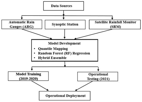
Figure 1. Study framework.

2.2. Study Area

The Cagayan de Oro River Basin (CDORB) is located in northern Mindanao, Philippines (8°15′–8°45′ N, 124°30′–125°15′ E), covering approximately 1521 km² [20] with elevations ranging from coastal areas near Cagayan de Oro City (<100 m) to the Kitanglad Range headwaters (>2000 m) (Figure 1). This steep elevation gradient creates distinct ecological zones visible in the land cover distribution: closed and open forests dominate the upper basin (>1000 m elevation), providing watershed protection; agricultural areas (rice, corn, and agroforestry systems) occupy the mid-to-lower elevations (200–800 m); grassland and shrubland represent deforested transitional zones; and built-up areas concentrate near the basin outlet in Cagayan de Oro City, the regional urban center. The basin’s rainfall monitoring network consists of one synoptic station and five Automated Rain Gauges (ARGs) distributed across the elevation gradient (Figure 2).

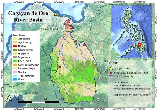
Figure 2. Study area and location of ARGs and Synoptic Station.

Based on satellite rainfall estimates for 2015–2023 extracted from the Google Earth Engine, CDORB receives a mean annual rainfall of 2994 ± 627 mm (CV = 21.0%), with annual totals ranging from 2188 mm to 3794 mm, a 73% difference (Table 1). Rainfall shows clear seasonality consistent with a Modified Coronas Type III climate [21]. The wet season (May–October) contributes 62% of annual rainfall, driven by the southwest monsoon and tropical cyclones, while the drier season contributes 38%. Monthly rainfall variability is substantial: 67–175%, with higher variability during the drier season. This pronounced interannual and intraannual variability [22], combined with documented gauge failures during extreme events and the basin’s history of flood disasters (Tropical Storm Sendong, 2011), makes the CDORB ideal for evaluating the temporal transferability of satellite rainfall correction methods under realistic operational constraints.

Table 1. Annual rainfall variability in CDORB (2015–2023).

Year	Rainfall (mm)	% of Mean	ENSO Phase
2015	2188	73%	El Niño
2016	2456	82%	Transitioning
2017	2891	97%	Neutral
2018	3124	104%	Neutral
2019	2978	99%	Neutral
2020	3267	109%	La Niña
2021	3794	127%	La Niña
2022	3156	105%	La Niña
2023	3098	103%	Neutral

2.3. Data Quality Control and Preprocessing

Quality control procedures were applied uniformly to both training and testing datasets. Negative rainfall values were removed as physically impossible measurements. Extreme values exceeding the 99th percentile were removed using percentile-based thresholds (67.09 mm for SRM, 58.27 mm for ARG). The decision to remove values exceeding the 99th percentile requires careful justification, given that extreme rainfall events are critical for flood warning systems. This threshold was applied specifically to remove measurement errors and data artifacts (such as instrument malfunctions, transmission errors, or sensor saturation) rather than legitimate heavy precipitation events. The 99th percentile threshold was selected through visual inspection of the data distribution and consultation with DOST-ASTI data quality protocols, which identified several anomalous readings exceeding physical plausibility for the basin’s climatology. Post-filtering, the dataset retained 97.9% of observations, confirming that only a small fraction of extreme outliers were removed. The correction methods were specifically evaluated on their ability to handle the remaining range of rainfall intensities (0–67 mm), which encompasses the operationally relevant spectrum for flood early warning in this basin.

Zero rainfall days were retained throughout all analyses despite constituting 46.7 percent of observations, ensuring operational realism since deployed systems must handle days without precipitation. The analysis framework treats each ARG station as an independent observation point, resulting in station-day records where each day’s rainfall is recorded separately for all five stations. For the comprehensive training period (January 2019–December 2020, 731 calendar days), this yielded 3655 potential station-day records. After quality control removed invalid measurements, 3579 valid station-day records were retained for model development.

2.4. Ground-Based Rainfall Measurements

Ground-based rainfall data served as the reference for developing and validating correction methods. Five Automated Rain Gauges (ARGs) within CDORB, managed by DOST-ASTI, provided the primary reference dataset. Each ARG uses tipping-bucket technology, recording rainfall at 10 or 15 min intervals, with built-in quality control systems that automatically verify data location, timestamp, value range, and internal consistency following PAGASA and DOST-ASTI guidelines. Measurements were aggregated into daily totals (mm/day).

The use of only five ARG stations in CDORB represents a realistic constraint rather than a limitation, as sparse gauge networks are typical in Philippine river basins due to equipment costs, maintenance challenges, and typhoon damage. To maximize statistical power while preserving spatial information, each ARG-satellite pair was treated as an independent observation point in the station-day framework. This approach is justified because (1) each ARG station captures spatially distinct rainfall characteristics based on its location within the basin (coastal lowlands vs. mountainous headwaters), (2) daily rainfall measurements at different stations exhibit low spatial autocorrelation beyond ~10 km in tropical convective systems, and (3) the pairing with corresponding satellite pixels ensures that each observation represents a unique satellite-ground comparison. The resulting 3579 station-day records after quality control provide sufficient sample size for robust correction model development while acknowledging that spatial coverage is limited by gauge availability. This station-based approach reflects operational realities and enables evaluation of correction methods under data constraints that actual flood warning systems must navigate.

Each of the five ARG stations was paired with its corresponding satellite pixel location, treating each ARG-satellite pair as an independent observation point. This station-based approach preserves spatial variability information while providing sufficient sample size for robust correction model development. For each day, rainfall measurements from all five ARG stations were compared with their corresponding satellite estimates, yielding station-day records as the fundamental analysis unit. Daily rainfall data from the El Salvador Synoptic Station (operated by PAGASA) were used to validate ARG network reliability through correlation analysis (Spearman’s ρ ≥ 0.70 threshold), confirming the ARG network provided dependable reference observations for correction model development.

2.5. Satellite-Based Rainfall Measurements

Satellite rainfall estimates were acquired through the Satellite Rainfall Monitoring (SRM) module developed by PHIVOLCS, combining data from NOAA’s NESDIS and JAXA’s Global Satellite Mapping of Precipitation (GSMaP). Daily rainfall values (mm/day) were collected for CDORB using the SRM interface. Virtual rain gauge (VRG) coordinates were manually matched to actual ARG locations. These matched coordinates enabled direct comparison between satellite estimates and spatially averaged ground observations at corresponding locations.

2.6. Correction Methods

Following validation, ARG data were used as the reference for evaluating and correcting SRM measurements. Three correction methods were implemented:

2.6.1. Quantile Mapping (QM)

Quantile Mapping corrects satellite rainfall by aligning its statistical distribution with ground-based observations using cumulative distribution functions (CDFs):

$${\mathrm{ŷ}}_{QM}= F_{ARG}^{-1}\left(F_{SRM}\left(x\right)\right)$$

(1)

where x is the uncorrected measurement, $F_{SRM}\left(x\right)$ converts it to a percentile rank, $F_{ARG}^{-1}$ maps this to the ground-based value, and ${\mathrm{ŷ}}_{QM}$ is the corrected estimate. QM represents a purely statistical approach that operates on relative rainfall rankings rather than absolute magnitudes.

2.6.2. Random Forest Regression (RF)

Random Forest builds multiple decision trees and averages predictions to capture complex, nonlinear relationships:

$${\mathrm{ŷ}}_{RF}= {\displaystyle \frac{1}{T}}{\sum }_{t=1}^T{h}_t\left(x\right)$$

(2)

where ${\mathrm{ŷ}}_{RF}$ is the predicted rainfall, $x$ represents input features (SRM value, day of year, month), $h_t\left(x\right)$ is each tree’s prediction, and T is the number of trees. Temporal features (day of year, month) were included to enable learning of seasonal patterns, including monsoon cycles and wet/dry season transitions. Hyperparameter optimization yielded the following: 400 trees, a maximum depth of 10, and a minimum of 5 samples per split (Table 2). RF represents a machine learning approach capable of learning complex correction patterns but potentially susceptible to overfitting training-period conditions.

Table 2. Optimal hyperparameter configuration for the Random Forest Regression (RF) model.

Parameter	Tested Values	Selected Values
N	100, 200, 300, 400	400
depth limits	5, 10, 20	10
minimum samples	2, 5, 10	5

2.6.3. Ensemble Model

The Hybrid Ensemble combines QM and RF using Ordinary Least Squares (OLS) regression to determine optimal weights:

$${\mathrm{ŷ}}_{ensemble}=\mathsf{\alpha }+{\mathsf{\beta }}_1 \times {\mathrm{ŷ}}_{QM}+{\mathsf{\beta }}_2 \times {\mathrm{ŷ}}_{RF}$$

(3)

where α is the intercept, β₁ and β₂ are statistically optimized weights, and ${\mathrm{ŷ}}_{ensemble}$ is the final corrected estimate. This hybrid approach attempts to balance QM’s distributional correction with RF’s adaptive learning capabilities.

2.7. Model Calibration Framework

2.7.1. Comprehensive Calibration (2019–2020)

All three correction methods were first calibrated using the complete 2019–2020 dataset (January 2019 to December 2020), comprising 3579 daily observations after quality control. This scenario represents ideal conditions where monitoring networks function continuously across both wet and dry monsoon phases, providing comprehensive coverage of rainfall variability. Models were evaluated on the same 2019–2020 training period to quantify calibration accuracy. Performance metrics included Root Mean Square Error (RMSE), Mean Absolute Error (MAE), Bias, Nash-Sutcliffe Efficiency (NSE), and Coefficient of Determination (R²).

2.7.2. Seasonal Stability Assessment

To evaluate whether corrections remain stable across different rainfall regimes within the calibration period, performance was assessed separately for the following:

• Dry season (January–April): lower rainfall frequency and intensity, dominated by shallow convection
• Wet season (May–December): higher rainfall frequency and intensity, dominated by deep convective systems

Seasonal disaggregation tested whether models trained on full-year data maintain consistent performance when applied to contrasting monsoon phases, which is essential for year-round operational deployment in flood early warning systems.

2.8. Temporal Transferability Assessment

2.8.1. Operational Testing Scenario

The critical test of operational viability is whether correction methods maintain accuracy when applied to future periods with different rainfall characteristics—particularly under realistic constraints where equipment failures limit calibration data availability. To simulate operational constraints typical of Philippine river basins, all models were retrained using only January–April 2019–2020 data. This reflects the reality in CDORB where the ARG network became non-operational after April 2020 due to equipment failures, a common scenario where typhoon damage creates multi-month monitoring gaps and flood early warning systems must function despite incomplete annual data coverage.

2.8.2. Independent Validation Period

Models trained on January–April 2019–2020 were then tested on January–April 2021, an independent future period exhibiting substantially different rainfall conditions. This regime-shift scenario tests whether corrections transfer reliably across years when natural interannual climate variability (influenced by ENSO phases and monsoon intensity fluctuations) alters rainfall characteristics. This design explicitly evaluates temporal transferability.

2.8.3. Transferability Metrics

Temporal transferability was quantified by comparing performance stability between training and testing periods. Performance stability metrics included the following:

• Absolute R² change (ΔR²) = R²_test − R²_train;
• Percentage R² change (%ΔR²) = [(R²_test − R²_train)/R²_train] × 100;
• Consistency of error metrics (RMSE, MAE, Bias) between training and testing;

Following the thresholds established in hydrological studies [23,24], a correction method was considered operationally viable if it met the following four criteria in both training and independent validation periods: R² ≥ 0.50 (adequate predictive skill), NSE ≥ 0.50 (acceptable model efficiency), RMSE < 10 mm/day (operationally acceptable error), and |Bias| < 30% (reasonable systematic error). Methods failing to meet these thresholds during independent validation were classified as unsuitable for operational deployment, regardless of training performance.

2.9. Evaluation Metrics

Statistical metrics included Root Mean Square Error (RMSE), Mean Absolute Error (MAE), Bias, Nash-Sutcliffe Efficiency (NSE), and Coefficient of Determination (R²). Performance classification followed thresholds established in hydrological studies [23,24], which are summarized in Table 3.

Table 3. Threshold classification for evaluation metrics.

Metric	Unsatisfactory	Satisfactory	Good	Very Good
R2	<0.50	0.50–0.75	0.75–0.90	>90
RMSE	>15 mm/day	10–15 mm/day	5–10 mm/day	<5 mm/day
MAE	>10 mm/day	6–10 mm/day	3–6 mm/day	<3 mm/day
NSE	≤0.50	0.50–0.65	0.65–0.75	>0.75
PBias	>±0.25	±15–25	±10–15	<10

2.10. Software and Code Availability

All analyses were conducted in Python 3.12.12 within the Google Colab environment (Google LLC, Mountain View, California, USA). The study utilized scikit-learn 1.6.1 for implementing Random Forest models, NumPy 2.0.2 for numerical computations, and SciPy 1.16.3 for statistical analyses. Python scripts for Quantile Mapping, Random Forest, and Hybrid Ensemble correction methods are available from the corresponding author upon reasonable request. QuantileTransformer from scikit-learn implemented Quantile Mapping with the number of quantiles adapted to sample size (100 quantiles for comprehensive training, 50 quantiles for seasonally limited operational training). RandomForestRegressor from scikit-learn implemented Random Forest with hyperparameters specified in Table 1. LinearRegression from scikit-learn implemented Ordinary Least Squares optimization for Hybrid Ensemble weight determination. All random processes used fixed random states (random_state = 42).

3. Results

3.1. Validation of ARG Reference Data

The ARG network showed strong agreement with the El Salvador Synoptic Station, with Spearman’s rank correlation coefficients ranging from ρ = 0.767 to 0.873 (Figure 3). Both datasets exhibited consistent seasonal transitions and synchronous rainfall peaks, confirming that ARGs reliably captured basin-wide rainfall behavior. These values exceed the ρ ≥ 0.70 threshold for hydrological network validation [23,24], establishing the ARG network as a dependable reference for satellite rainfall correction.

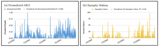
Figure 3. Temporal comparison of normalized rainfall between averaged (a) ARG network observations and (b) synoptic station.

3.2. Baseline Satellite Performance

The uncorrected SRM exhibited severe systematic biases compared with ARG observations (Figure 4). The product captured only about half the magnitude of observed rainfall (slope = 0.506, intercept = 4.387 mm), underestimating moderate-to-heavy precipitation while overestimating light rainfall. Points below the 1:1 line at high intensities (>35 mm/day) highlight severe underestimation of heavy rainfall critical for flood warnings, while points above the line at low intensities (<10 mm/day) show overestimation of light rainfall. Weak correlation and large scatter confirm poor reliability for operational applications.

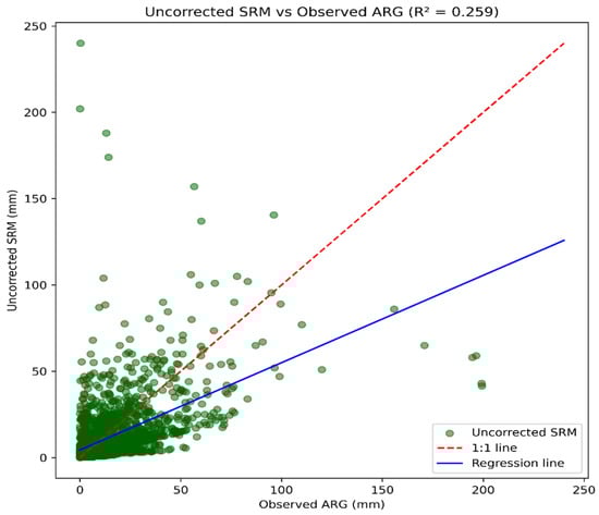
Figure 4. Scatter plot comparing ARG observations versus uncorrected SRM estimates.

3.3. Correction Model Performance (2019–2020 Training)

All three correction methods were trained on the complete 2019–2020 dataset comprising 3579 daily records after quality control. Table 4 summarizes the performance metrics, and Figure 5 illustrates the distribution alignment achieved by each correction method, showing how QM, RF, and Hybrid transform the raw SRM distribution to match ARG observations.

Table 4. Comprehensive training performance (2019–2020).

Model	RMSE (mm)	MAE (mm)	Bias (mm)	NSE	R2
QM	8.27	4.90	−0.005	0.25	0.25
RF	5.17	2.72	−0.005	0.71	0.71
Hybrid Ensemble	4.69	2.85	~0	0.76	0.76

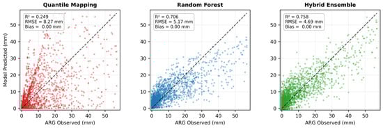
Figure 5. Scatter plots showing rainfall distribution alignment for QM, RF, and Hybrid.

3.3.1. Quantile Mapping

Quantile Mapping achieved R² = 0.25 and NSE = 0.25 during comprehensive training, which represents satisfactory performance for a purely distributional correction method. The approach successfully reduced systematic bias to near-zero (−0.01 mm) by aligning the satellite rainfall distribution with ground observations. RMSE decreased to 8.27 mm and MAE to 3.90 mm, both falling within acceptable ranges for operational applications. While QM’s correlation was lower than the machine learning methods, this moderate performance reflected its straightforward percentile-based correction mechanism that operates on rainfall rank order rather than learning complex patterns from temporal features.

Figure 6 illustrates how QM works through empirical cumulative distribution functions. The left panel shows the CDFs for both SRM satellite estimates and ARG ground observations, with quartile thresholds marked at the 25th, 50th, and 75th percentiles. The 95% confidence band around the SRM CDF indicates the statistical uncertainty in the distribution. The right panel demonstrates the quantile-quantile mapping process, where each rainfall value from the satellite distribution is mapped to the corresponding percentile value in the ground observation distribution. The colored arrows at quartile positions show how SRM values are adjusted to match ARG percentile values, ensuring that corrected values maintain proper statistical characteristics across all rainfall intensities.

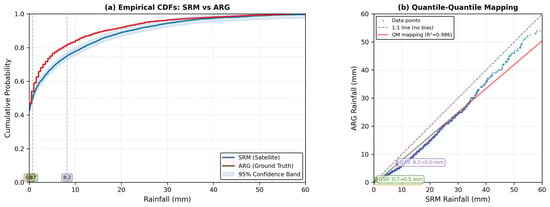
Figure 6. Empirical CDF of SRM estimates with quartile thresholds and 95% confidence band.

3.3.2. Random Forest Regression

Random Forest achieved substantially better performance than QM during comprehensive training, with R² = 0.71 and NSE = 0.71. RMSE dropped to 5.17 mm and MAE to 2.72 mm, both classified as “Very Good”. The model maintained near-zero bias (0.01 mm), indicating no systematic over- or under-prediction. As shown in Figure 6, RF-corrected values aligned closely with observed rainfall across the full intensity range from light to heavy precipitation. The inclusion of temporal features (day of year and month) enabled RF to learn seasonal correction patterns specific to monsoon cycles and wet/dry season transitions, contributing to its superior training accuracy.

3.3.3. Hybrid Ensemble

The Hybrid Ensemble achieved the highest training performance among all methods, with R² = 0.76 and NSE = 0.76. RMSE was 4.69 mm and MAE was 2.85 mm, both in the “Very Good” classification range. Bias remained essentially zero (0.00 mm). Figure 6 shows that Hybrid predictions clustered most tightly around the 1:1 line, indicating accurate reproduction of observed rainfall magnitudes. The OLS regression that combined QM and RF outputs assigned heavy weight to RF (β_RF = 1.60) while giving minimal negative weight to QM (β_QM = −0.37), meaning the Hybrid method primarily relied on RF’s pattern-learning capabilities with only marginal contribution from QM’s distributional correction.

3.4. Seasonal Stability

Model performance was evaluated separately for the dry season (January–April) and wet season (May–December) within the 2019–2020 calibration period (Table 5 and Table 6). This seasonal stability assessment serves as an intermediate diagnostic to evaluate whether the correction methods exhibit sensitivity to different monsoon phases within the training period, prior to testing full interannual transferability.

Table 5. Dry season performance (January–April 2019–2020).

Model	RMSE (mm)	MAE (mm)	Bias (mm)	R2	NSE
QM	4.42	1.29	0.29	0.22	0.22
RF	2.21	0.76	0.04	0.80	0.80
Hybrid	2.19	1.36	−0.83	0.81	0.81

Table 6. Wet season performance (May–October 2019–2020).

Model	RMSE (mm)	MAE (mm)	Bias (mm)	R2	NSE
QM	9.62	5.19	−0.15	0.19	0.19
RF	6.12	3.69	−0.01	0.67	0.67
Hybrid	5.52	3.59	0.41	0.73	0.73

During the dry season (1188 days, mean rainfall = 1.42 mm/day, 25.9% rainy days), all three methods performed reasonably well, with RF and Hybrid achieving particularly strong results (R² > 0.80, RMSE < 2.3 mm). QM showed moderate performance (R² = 0.22) consistent with its overall training behavior. During the wet season (2391 days, mean rainfall = 6.59 mm/day, 67.0% rainy days), all methods showed some performance degradation due to the higher rainfall variability and intensity. QM maintained relatively consistent performance across seasons (R² = 0.22 dry, 0.19 wet), while RF and Hybrid showed larger seasonal differences.

Figure 7 shows RMSE values across seasons for all correction methods. All methods exhibited higher errors during the wet season compared to the dry season. Quantile Mapping showed RMSE of 4.42 mm during the dry season increasing to 9.62 mm during the wet season. Random Forest demonstrated RMSE of 2.21 mm (dry season) increasing to 6.13 mm (wet season). The Hybrid Ensemble showed RMSE of 2.19 mm (dry season) increasing to 5.53 mm (wet season). Random Forest and Hybrid Ensemble maintained lower absolute errors than Quantile Mapping in both seasons, though all methods showed substantial performance degradation during wetter conditions.

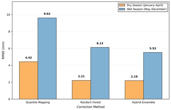
Figure 7. RMSE comparison across seasons for Raw SRM, QM, RF, and Hybrid models.

3.5. Temporal Transferability and Operational Viability

3.5.1. Testing Scenario Result

To simulate realistic operational constraints, all models were retrained using only data from the dry season months of January–April 2019–2020, reflecting the reality that CDORB’s ARG network became non-operational after April 2020. Models were then tested on January–April 2021 to evaluate performance on an independent future period. Importantly, the 2021 test period experienced substantially wetter conditions than the training period, with mean rainfall of 3.13 mm/day compared to 1.42 mm/day during training. This created a regime-shift scenario that explicitly tested whether correction methods remain reliable when future rainfall patterns differ from calibration conditions.

3.5.2. Training Performance on Seasonally Limited Data

When trained only on dry-season data, all three methods achieved reasonable performance on the training period itself. Table 7 summarizes the operational training performance metrics.

Table 7. Operational training performance (January–April 2019–2020).

Model	RMSE (mm)	MAE (mm)	Bias (mm)	R2	NSE
QM	3.78	1.12	2.12	0.43	0.43
RF	2.14	0.69	1.03	0.82	0.82
Hybrid	2.01	0.72	−5.42	0.84	0.84

QM reached R² = 0.43 with RMSE = 3.78 mm, classified as “Satisfactory” performance. RF demonstrated excellent training accuracy with R² = 0.82 and RMSE = 2.14 mm. The Hybrid Ensemble achieved the highest training performance with R² = 0.84 and RMSE = 2.01 mm.

3.5.3. Testing Performance Under Regime Shift (January–April 2021)

The critical test of operational viability occurred when models trained on January–April 2019–2020 were applied to the independent 2021 test period with substantially different rainfall characteristics. This regime-shift scenario revealed dramatic differences in temporal transferability among the three correction methods. Table 8 presents the operational testing performance metrics.

Table 8. Operational testing performance (January–April 2021).

Model	RMSE (mm)	MAE (mm)	Bias (mm)	R2	NSE
QM	5.23	2.43	−0.61	0.52	0.52
RF	5.63	2.60	−0.64	0.45	0.45
Hybrid	5.85	2.77	−0.53	0.41	0.41

Table 7 shows performance rankings reversed completely. QM achieved R² = 0.53, which is above the operational threshold, while RF and Hybrid declined to R² = 0.46 and 0.41, which are below the threshold.

Figure 8 shows scatter plots comparing training and testing performance for each method. QM maintained consistent scatter patterns in both periods, with points distributed similarly around the 1:1 line in training and testing. RF showed tight clustering during training but severe scatter during testing, with many predictions deviating substantially from observed values. Hybrid exhibited similar degradation, with the tight training-period fit completely disappearing during testing.

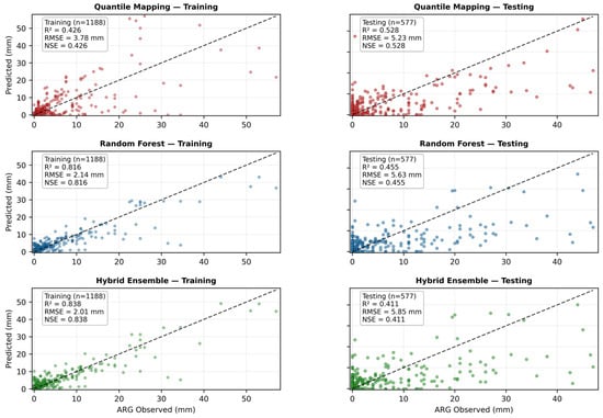
Figure 8. Scatter plots comparing ARG observations versus model predictions during January–April 2021 testing.

Figure 9 shows the quantification of the performance changes between training and testing. The left panel shows ΔR² values: QM improved by +0.10, while RF declined by −0.36 and Hybrid declined by −0.43. The right panel shows ΔRMSE values: QM’s error increased by 1.45 mm, RF’s error increased by 3.49 mm, and Hybrid’s error increased by 3.84 mm.

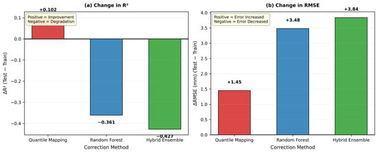
Figure 9. Performance comparison between training (January–April 2019–2020) and testing (January–April 2021) periods, showing R² change (ΔR²) for each correction method.

Lastly, Figure 10 summarizes operational viability against the R² ≥ 0.50 threshold. Only QM maintained performance above this threshold during independent testing, marked with a green checkmark. Both RF and Hybrid fell below the threshold, marked with red X symbols, indicating they failed to meet operational reliability standards despite their excellent training performance.

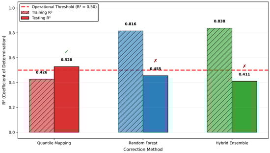
Figure 10. Operational viability performance of QM, RF, and Hybrid Ensemble.

4. Discussion

4.1. Why Quantile Mapping Maintained Reliability While Machine Learning Failed

The operational testing revealed fundamental differences in how correction methods handle rainfall regime shifts. Quantile Mapping succeeded because it operates on percentile ranks rather than absolute rainfall magnitudes. When QM maps the 50th percentile of satellite data to the 50th percentile of ground observations, this correction remains valid whether that percentile corresponds to 5 mm during training or 10 mm during testing. When 2021 exhibited wetter conditions (120% higher mean rainfall, 33% increased rainy-day frequency), QM automatically adapted because the percentile mapping function still worked—the wetter regime actually improved performance slightly (R² from 0.43 to 0.53) because more pronounced rainfall events provided better percentile separation.

Random Forest and Hybrid Ensemble failed because they learned magnitude-specific correction rules during training. When trained on dry-season data (mean = 1.42 mm, 25.9% rainy days), RF constructed decision trees optimized for those specific conditions. The temporal features (day of year, month) helped RF learn seasonal patterns calibrated to 2019–2020 rainfall characteristics. When confronted with 2021’s wetter regime (mean = 3.13 mm, 33.3% rainy days), these decision rules became invalid—RF had no mechanism to extrapolate beyond its training distribution, resulting in the 44% R² decline. The Hybrid Ensemble’s more severe failure (51% decline) occurred because the OLS optimization prioritized RF’s training accuracy (β_RF = 1.60, β_QM = −0.37), meaning it relied almost entirely on RF while actually subtracting QM’s contribution. When RF failed, minimal QM weight provided no compensatory stability.

These findings align with recent studies highlighting limitations of machine learning temporal transferability. A study Juel et al. [25] reported that Random Forest classification accuracy decreased when models were applied to different time periods or study areas, consistent with our regime-shift results. For precipitation applications specifically, recent work in Ghana and Zambia [26] using continuous temporal splits (training on 1983–2000, testing on 2001–2022) revealed a high discrepancy in rainfall characteristics between periods, attributable to climate change and long-term variability. Their findings that Support Vector Regression (SVR) and Gaussian Process Regression (GPR) showed inconsistent transferability across different locations mirror our observation that magnitude-specific learning fails under changing conditions.

The two-year calibration period (2019–2020) may not fully encompass interannual variability driven by ENSO oscillations or longer-term climate trends. Because QM relies on statistical distribution matching rather than event-scale physical learning, it may underperform in reproducing short-duration extreme rainfall and highly localized convective events, especially when such extremes are poorly represented in calibration data. QM has been applied for bias correction in tropical regions [27], mountainous terrain, and arid environments [28], though it often exhibits lower calibration accuracy than ML approaches under stationary conditions where complex nonlinear relationships can be learned more effectively [29].

The validation period (2021) demonstrated that QM corrections remained stable outside the training window, but this represents only one additional year. Cannon et al. [30] emphasized that quantile mapping algorithms must be evaluated not only on calibration performance but also on their ability to preserve projected changes under non-stationary conditions. Future work should extend both the calibration and validation periods to 5–10 years to capture broader variability including extreme wet and dry years. Independent validation using spatially withheld stations or split-sample testing across different ENSO phases would further strengthen confidence in transferability [14]. However, these limitations must be weighed against QM’s demonstrated operational advantages: computational efficiency, minimal data requirements, and sustained performance under regime shifts observed even with this limited calibration window.

4.2. Operational Deployment Recommendations

Based on these results, Quantile Mapping emerges as the only operationally viable correction method for data-limited tropical basins like CDORB. QM maintained performance above operational thresholds when tested under realistic regime-shift conditions, and its percentile-based approach transferred effectively across years without requiring retraining.

The success of QM occurred within specific conditions: a tropical maritime climate with a Type III rainfall distribution, a moderate-elevation basin with mixed convective/orographic precipitation, SRM’s NESDIS-GSMaP fusion algorithm, and a sparse five-station network. QM’s robustness may be particularly advantageous where equipment failures are common and rapid deployment is prioritized. Studies in Vietnam’s Lam River Basin [31] and Indonesia [32] similarly demonstrated QM effectiveness for enhancing satellite precipitation in data-limited tropical environments, confirming the broader applicability of our findings across Southeast Asian monsoon regions. However, in regions with denser networks or longer data records, machine learning approaches might achieve better transferability if trained on diverse hydroclimatic conditions spanning multiple ENSO cycles. The key insight is that operational validation frameworks using temporal splits and regime-shift scenarios are essential to distinguish genuine transferability from cross-validation performance. Traditional random train-test splits that assume stationary relationships over time [9,10] systematically overestimate operational reliability, as demonstrated by the dramatic performance declines we observed.

4.3. Pathways for Enhancing Machine Learning Transferability

While Random Forest and Hybrid Ensemble failed under the regime-shift scenario in this study, several approaches could potentially improve machine learning transferability for future applications. First, training on diverse data spanning 5–10 years with varied rainfall regimes (wet/dry years, different ENSO phases) could enable ML methods to learn generalizable patterns rather than magnitude-specific rules calibrated to limited conditions [33]. Second, physics-informed feature engineering incorporating atmospheric variables (moisture content, pressure gradients, synoptic patterns) might provide more stable correction signals than temporal indicators alone. Third, ensemble strategies with time-varying weights that shift between QM and ML based on detected regime characteristics could preserve operational reliability while leveraging pattern learning. Fourth, uncertainty quantification methods that flag extrapolation beyond training conditions could trigger automatic fallback to QM when predictions become unreliable. However, these enhancements require substantially more data, computational resources, and technical complexity than QM’s straightforward approach. For immediate operational deployment in data-limited basins, QM remains the practical choice, while long-term research should investigate whether enhanced ML methods can achieve both high accuracy and robust transferability.

5. Conclusions

This study evaluated whether satellite rainfall correction methods maintain operational reliability when applied to future periods with different rainfall characteristics under realistic data constraints. Three key findings emerged for flood early warning systems in data-limited tropical basins.

First, training accuracy was shown to be a poor predictor of operational reliability. The Random Forest and Hybrid Ensemble methods achieved excellent calibration performance but experienced performance declines (44–51%), falling below operational thresholds. In contrast, Quantile Mapping maintained satisfactory performance despite only moderate training accuracy. Second, percentile-based correction methods demonstrated greater reliability to rainfall regime shifts than magnitude-specific learning approaches. Quantile Mapping operates on rainfall rank order rather than absolute magnitudes, allowing it to adapt automatically when the 2021 validation period exhibited approximately 120% higher mean rainfall without requiring recalibration. Machine learning methods, by contrast, learned correction rules optimized for training-period magnitudes and failed to extrapolate when rainfall characteristics changed. Third, operational deployment requires correction methods that remain reliable under incomplete calibration data. When models were trained using only January–April data to simulate equipment failures, Quantile Mapping was the only method that maintained operational viability during independent testing, reflecting common real-world scenarios in which typhoon damage creates prolonged monitoring gaps.

For Philippine river basins and similar data-limited tropical basins with sparse gauge networks and high interannual rainfall variability, Quantile Mapping emerges as the most operationally viable correction method under the conditions tested in this study. A recommended operational protocol is to train Quantile Mapping using available data, even if seasonally limited, apply corrections continuously without retraining, and validate performance when new data become available, using established hydrological performance thresholds (R² ≥ 0.50, NSE ≥ 0.50, RMSE < 10 mm/day). More broadly, this study demonstrates that operational validation frameworks using temporal splits and regime-shift scenarios are essential for model selection, as calibration performance alone can be misleading. While the two-year calibration period represents a limitation, future studies should extend validation to 5–10 years to capture broader hydroclimatic variability and different ENSO phases. Nevertheless, Quantile Mapping’s demonstrated operational advantages—computational efficiency, minimal data requirements, and sustained performance under regime shifts—make it a practical and defensible choice for operational flood early warning systems in data-limited tropical regions where reliable rainfall information is critical for risk reduction.

References

- New, M.; Todd, M.; Hulme, M.; Jones, P. Precipitation measurements and trends in the twentieth century. Int. J. Climatol. 2001, 21, 1889–1922. [Google Scholar] [CrossRef]
- Kidd, C.; Becker, A.; Huffman, G.J.; Muller, C.L.; Joe, P.; Skofronick-Jackson, G.; Kirschbaum, D.B. So, how much of the Earth’s surface is covered by rain gauges? Bull. Am. Meteorol. Soc. 2017, 98, 69–78. [Google Scholar] [CrossRef] [PubMed]
- Huffman, G.J.; Bolvin, D.T.; Braithwaite, D.; Hsu, K.; Joyce, R.; Xie, P.; Yoo, S.H. NASA Global Precipitation Measurement (GPM) Integrated Multi-satellitE Retrievals for GPM (IMERG). Algorithm Theor. Basis Doc. (ATBD) Version 2015, 4, 30. [Google Scholar]
- Kidd, C.; Levizzani, V. Status of satellite precipitation retrievals. Hydrol. Earth Syst. Sci. 2011, 15, 1109–1116. [Google Scholar] [CrossRef]
- Sun, Q.; Miao, C.; Duan, Q.; Ashouri, H.; Sorooshian, S.; Hsu, K.L. A review of global precipitation data sets: Data sources, estimation, and intercomparisons. Rev. Geophys. 2018, 56, 79–107. [Google Scholar] [CrossRef]
- Tang, G.; Clark, M.P.; Papalexiou, S.M.; Ma, Z.; Hong, Y. Have satellite precipitation products improved over last two decades? A comprehensive comparison of GPM IMERG with nine satellite and reanalysis datasets. Remote Sens. Environ. 2020, 240, 111697. [Google Scholar] [CrossRef]
- Fei, T.; Huang, B.; Wang, X.; Zhu, J.; Chen, Y.; Wang, H.; Zhang, W. A hybrid deep learning model for the bias correction of SST numerical forecast products using satellite data. Remote Sens. 2022, 14, 1339. [Google Scholar] [CrossRef]
- Wang, C. Calibration in Deep Learning: A Survey of the State-of-the-Art. arXiv 2023, arXiv:2308.01222. [Google Scholar] [CrossRef]
- Beck, H.E.; Pan, M.; Roy, T.; Weedon, G.P.; Pappenberger, F.; van Dijk, A.I.J.M.; Huffman, G.J.; Adler, R.F.; Wood, E.F. Daily evaluation of 26 precipitation datasets using Stage-IV gauge-radar data for the CONUS. Hydrol. Earth Syst. Sci. 2019, 23, 207–224. [Google Scholar] [CrossRef]
- Tan, M.L.; Armanuos, A.M.; Ahmadianfar, I.; Demir, V.; Heddam, S.; Al-Areeq, A.M.; Abba, S.I.; Halder, B.; Cagan Kilinc, H.; Yaseen, Z.M. Evaluation of NASA POWER and ERA5-Land for estimating tropical precipitation and temperature extremes. J. Hydrol. 2023, 624, 129940. [Google Scholar] [CrossRef]
- Lu, M.; Song, X.; Yang, N.; Wu, W.; Deng, S. Spatial and temporal variations in rainfall seasonality and underlying climatic causes in the eastern China monsoon region. Water 2025, 17, 522. [Google Scholar] [CrossRef]
- Kubota, T.; Aonashi, K.; Ushio, T.; Shige, S.; Takayabu, Y.N.; Kachi, M.; Arai, Y.; Tashima, T.; Masaki, T.; Kawamoto, N.; et al. Global Satellite Mapping of Precipitation (GSMaP) products in the GPM era. Satell. Precip. Meas. 2020, 1, 355–373. [Google Scholar] [CrossRef]
- Joyce, R.J.; Janowiak, J.E.; Arkin, P.A.; Xie, P. CMORPH: A method that produces global precipitation estimates from passive microwave and infrared data at high spatial and temporal resolution. J. Hydrometeorol. 2004, 5, 487–503. [Google Scholar] [CrossRef]
- Stephens, C.M.; Pham, H.T.; Marshall, L.A.; Johnson, F.M. Which rainfall errors can hydrologic models handle? Implications for using satellite-derived products in sparsely gauged catchments. Water Resour. Res. 2022, 58, e2020WR029331. [Google Scholar] [CrossRef]
- Maggioni, V.; Massari, C. On the performance of satellite precipitation products in riverine flood modeling: A review. J. Hydrol. 2018, 558, 214–224. [Google Scholar] [CrossRef]
- Reichstein, M.; Camps-Valls, G.; Stevens, B.; Jung, M.; Denzler, J.; Carvalhais, N.; Prabhat, F. Deep learning and process understanding for data-driven Earth system science. Nature 2019, 566, 195–204. [Google Scholar] [CrossRef]
- Bergen, K.J.; Johnson, P.A.; de Hoop, M.V.; Beroza, G.C. Machine learning for data-driven discovery in solid Earth geoscience. Science 2019, 363, eaau0323. [Google Scholar] [CrossRef]
- Sham, F.A.F.; El-Shafie, A.; Jaafar, W.Z.B.W.; Adarsh, S.; Sherif, M.; Ahmed, A.N. Improving rainfall forecasting using deep learning data fusing model approach for observed and climate change data. Sci. Rep. 2025, 15, 27872. [Google Scholar] [CrossRef]
- NDRRMC. Final Report on Tropical Storm Sendong (Washi); National Disaster Risk Reduction and Management Council: Manila, Philippines, 2011.
- NAMRIA. Topographic Map of Northern Mindanao. Available online: https://www.namria.gov.ph/downloads.aspx (accessed on 24 November 2025).
- PAGASA. Climate of the Philippines. Available online: https://www.pagasa.dost.gov.ph/information/climate-philippines (accessed on 24 November 2025).
- PAGASA. Climatological Normals. Available online: https://www.pagasa.dost.gov.ph/climate/climatological-normals (accessed on 24 November 2025).
- Moriasi, D.N.; Arnold, J.G.; Van Liew, M.W.; Bingner, R.L.; Harmel, R.D.; Veith, T.L. Model evaluation guidelines for systematic quantification of accuracy in watershed simulations. Trans. ASABE 2007, 50, 885–900. [Google Scholar] [CrossRef]
- Gebregiorgis, A.S.; Hossain, F. Understanding the dependence of satellite rainfall uncertainty on topography and climate for hydrologic model simulation. IEEE Trans. Geosci. Remote Sens. 2014, 51, 704–718. [Google Scholar] [CrossRef]
- Juel, A.; Groom, G.B.; Svenning, J.; Ejrnæs, R. Spatial application of Random Forest models for fine-scale coastal vegetation classification using object based analysis of aerial orthophoto and DEM data. Int. J. Appl. Earth Obs. Geoinf. 2015, 42, 106–114. [Google Scholar] [CrossRef]
- Bagiliko, J.; Stern, D.; Torgbor, F.F.; Parsons, D.; Ansah, S.O.; Ndanguza, D. Bias correction of satellite and reanalysis products for daily rainfall occurrence and intensity. arXiv 2025, arXiv:2510.27456. [Google Scholar] [CrossRef]
- Tong, Y.; Gao, X.; Han, Z.; Xu, Y.; Xu, Y.; Giorgi, F. Bias correction of temperature and precipitation over China for RCM simulations using the QM and QDM methods. Clim. Dyn. 2020, 57, 1425–1443. [Google Scholar] [CrossRef]
- Elsebaie, I.H.; Kawara, A.Q.; Alharbi, R.; Alnahit, A.O. Bias Correction Methods Applied to Satellite Rainfall Products over the Western Part of Saudi Arabia. Atmosphere 2025, 16, 772. [Google Scholar] [CrossRef]
- Hao, Z.; Hao, F.; Singh, V.P.; Ouyang, W.; Cheng, H. An integrated package for drought monitoring, prediction and analysis to aid drought modeling and assessment. Environ. Model. Softw. 2017, 91, 199–209. [Google Scholar] [CrossRef]
- Cannon, A.J.; Sobie, S.R.; Murdock, T.Q. Bias Correction of GCM precipitation by quantile mapping: How well do methods preserve changes in quantiles and extremes? J. Clim. 2015, 28, 6938–6959. [Google Scholar] [CrossRef]
- Nguyen, N.Y.; Anh, T.N.; Nguyen, H.D.; Dang, D.K. Quantile mapping technique for enhancing satellite-derived precipitation data in hydrological modelling: A case study of the Lam River Basin, Vietnam. J. Hydroinform. 2024, 26, 2026–2044. [Google Scholar] [CrossRef]
- Simanjuntak, F.; Jamaluddin, I.; Lin, T.; Siahaan, H.A.W.; Chen, Y. Rainfall Forecast Using Machine Learning with High Spatiotemporal Satellite Imagery Every 10 Minutes. Remote Sens. 2022, 14, 5950. [Google Scholar] [CrossRef]
- Baez-Villanueva, O.M.; Zambrano-Bigiarini, M.; Ribbe, L.; Nauditt, A.; Giraldo-Osorio, J.D.; Thinh, N.X. Temporal and spatial evaluation of satellite rainfall estimates over different regions in Latin-America. Atmos. Res. 2020, 213, 34–50. [Google Scholar] [CrossRef]
Disclaimer/Publisher’s Note: The statements, opinions and data contained in all publications are solely those of the individual author(s) and contributor(s) and not of MDPI and/or the editor(s). MDPI and/or the editor(s) disclaim responsibility for any injury to people or property resulting from any ideas, methods, instructions or products referred to in the content. |
© 2026 by the authors. Licensee MDPI, Basel, Switzerland. This article is an open access article distributed under the terms and conditions of the Creative Commons Attribution (CC BY) license.