Abstract
The complex terrain of the Qinghai–Tibetan Plateau (QTP) makes low-level wind shear (LLWS) detection challenging. Using May–September 2023 high-resolution Doppler Wind Lidar (DWL) observations, this study analyzed the spatiotemporal characteristics of LLWS and proposed an optimized detection algorithm. A key novelty of this work lies in the development of a hybrid physical–statistical detection scheme that combines horizontal divergence with logistic regression to dynamically modulate the shear field. This approach effectively reduces noise-induced false alarms in complex plateau terrain. The results show that LLWS occurred mainly near the surface at night in June, while in September it appeared more frequently during daytime throughout the boundary layer. Horizontally, the dominant directions of LLWS shifted seasonally from northwest and west in June to south and east in September. The proposed optimization method effectively suppressed false alarms, reducing moderate and strong LLWS frequencies by 30–40%. In June, optimization significantly reduced spurious detections of LLWS in the northeast and southwest. The frequency of LLWS in the northeast direction was reduced by up to 0.03. In September, scattered shear was removed and strong shear became more organized in the southeast, while southwest shear frequency decreased by up to 0.04, confirming LLWS patterns and method effectiveness.
1. Introduction
Low-level wind shear (LLWS) refers to sudden changes in wind speed or direction within a few hundred meters of the ground. It is important for aviation safety, particularly during take-off and landing. LLWS can cause abrupt changes in altitude, speed, and lift, increasing the risk of loss of control [1,2]. Research by the International Civil Aviation Organization (ICAO) indicates that LLWS has directly contributed to several air accidents, resulting in hundreds of casualties. This highlights the urgent need for research and monitoring of LLWS [3].
In recent years, global research on LLWS has advanced significantly, focusing on both physical mechanisms and technical detection improvements. High-resolution observation systems, such as Doppler Wind Lidar (DWL), have enabled accurate monitoring of near-surface wind fields and provided reliable data support for LLWS warning systems [4,5,6]. For example, at Hong Kong International Airport, comprehensive DWL-based studies have examined LLWS associated with diverse weather phenomena, including foehn winds [7], tropical cyclones [8], downbursts [9], gust fronts [10], low-level jet streams [11], and terrain-induced wind shear [12,13]. Similar efforts have been carried out at Beijing Capital International Airport using pulsed coherent Doppler lidar [14,15], and at other international airports such as Nice Côte d’Azur [16], Taiwan’s Taoyuan [17], Guarulhos [18], and Frankfurt and Munich [19].
Parallel to observational advancements, significant progress has been made in the computational and algorithmic aspects of LLWS detection. Traditional signal-processing approaches have evolved into more sophisticated schemes that integrate physical modeling, filtering, and machine learning. For instance, Zhao and Shan proposed a Doppler lidar–based wind shear detection algorithm using a shear intensity factor, which enhanced weak-shear identification and reduced false alarm rates [20]. Deep learning techniques such as Temporal Convolutional Networks (TCN) have been introduced for LLWS prediction based on surface anemometer networks, achieving higher accuracy and lower false alarm ratios than traditional methods [21]. Earlier methodological frameworks, including Kalman filter–based predictive wind shear detection [22] and radar-based shear identification systems [23], laid the foundation for current algorithm optimization and sensor fusion applications. These developments collectively demonstrate that improving LLWS computation and reducing false alarms are becoming central goals in modern aviation meteorology.
Despite these advancements, existing LLWS detection methods still face notable limitations. Many algorithms show high false-alarm rates in complex or high-altitude terrain, and data-driven models often require large training datasets that are unavailable at plateau airports. As a result, accurately separating true shear signals from noise remains a key unresolved challenge. In mainland China, an analysis of LLWS reports from 2016 to 2020 indicated that airports frequently affected by LLWS are often located in areas with complex terrain or elevated topography [24]. Therefore, optimizing LLWS calculation methods and developing adaptive algorithms that enhance accuracy while minimizing false alarms are essential for improving forecasting and operational safety in such regions. To address this gap, this study introduces a hybrid divergence–logistic regression algorithm that dynamically adjusts the shear field and improves detection reliability under complex terrain conditions. The remainder of this paper is structured as follows. Section 2 outlines the datasets and the methodological framework used in this study. Section 3 presents the results of wind field, wind shear, and circulation analyses, and discusses the typical shear processes observed in summer and fall. Section 4 concludes by highlighting the improved LLWS detection achieved through the proposed divergence-based optimization algorithm. The major contributions of this study are summarized as follows:
- 1.
- Developed a combined divergence–logistic regression algorithm to reduce LLWS false alarms;
- 2.
- Revealed diurnal, seasonal, and vertical LLWS patterns at Lhasa Gonggar Airport;
- 3.
- Linked LLWS occurrence to key synoptic circulation patterns using ERA5 and clustering.
The following section introduces the observational data and methodological framework used in this study, including the site characteristics, clustering approach, shear calculation, and optimization procedures. The abbreviations and symbols used in this study are summarized in Appendix A.
2. Data and Methods
2.1. Site and Data
The Lhasa Gonggar Airport (ZULS), nestled in the southeast of the QTP, is located at an elevation of 3600 m (Figure 1). The runway alignment was built between two narrow mountain ranges with elevations up to 7000 m. As a result of the rugged terrain, the ZULS is subject to low-level wind shear under diverse weather conditions. To ensure accurate and comprehensive observations of the wind field, the DWL was used to measure the wind speed and wind direction by emitting a laser beam and analyzing its scattering signals after its interaction with microparticles or gas molecules in the atmosphere [25,26]. The two common modes are the plan-position-indicator (PPI) scan and the Doppler-beam-swinging (DBS) scan. Specific scanning parameters were configured as follows. (1) The PPI mode employed 3° elevation angles in this study to capture wind conditions near arrival and departure paths. Moreover, the horizontal azimuth scan was conducted with a 3° step size, completing a full 360° scan in approximately 180 s, and its range resolution was 100 m, ensuring high spatial detail in wind measurements over relatively large distances. (2) The DBS mode, the lidar’s antenna obtained the vertical wind speed structure, with a vertical resolution of 28 or 29 m. This fine vertical resolution enhanced the precision of wind profile measurements.
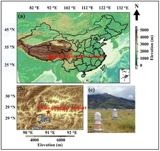
Figure 1.
Location of QTP (a) and surrounding terrain of the observation site (red pentagram) (b) and outdoor view of the Doppler wind Lidar (DWL) (c).
In addition, the reanalysis dataset used in this study was sourced from the European Centre for Medium-Range Weather Forecasts (ECMWF) ERA5, which provided hourly reanalysis data. This dataset included sea level pressure, 500 hPa u-wind and v-wind, and 500 hPa geopotential height. The time range covered was from 20 May to 30 September 2023, with data collected daily at 14 LT and 20 LT. The data was presented in 0.25-degree by 0.25-degree grids, updated every hour.
2.2. Cluster Method
The goal of K-means clustering was to group the samples according to their characteristics [27]. To identify the dominant large-scale atmospheric circulation regimes associated with wind shear, a K-means clustering analysis was applied to the standardized meteorological fields. The entire procedure consists of (1) variable standardization, (2) determination of the optimal number of clusters, and (3) iterative assignment and update steps.
- (1)
- Standardization of variables
All variables were standardized to remove unit effects:
where is the original variable, is its mean, is its standard deviation, and is the standardized variable.
- (2)
- Determination of the optimal number of clusters
The optimal cluster number K was determined using the elbow method and the silhouette coefficient:
where is cluster k, μk is its centroid, and denotes Euclidean distance.
where a(i) and b(i) are the intra- and nearest inter-cluster mean distances of sample i, respectively.
Figure 2 presents the two metrics used to determine the optimal number of clusters: (a) the within-cluster sum of squared errors (SSE) from the elbow method and (b) the silhouette coefficient. The SSE curve decreases monotonically with increasing K and shows a noticeable change in slope around K = 5, indicating that the marginal reduction in within-cluster variance becomes smaller beyond this point. However, the silhouette coefficient reaches its maximum at K = 4, suggesting that the balance between within-cluster compactness and between-cluster separation is optimal when using four clusters. Considering both metrics together, as well as the physical interpretability and stability of the resulting patterns, we selected K = 4 as the optimal number of clusters. Although SSE continues to decrease at K = 5, the improvement is marginal, and the additional cluster tends to over-partition existing patterns without providing clearer physical meaning.
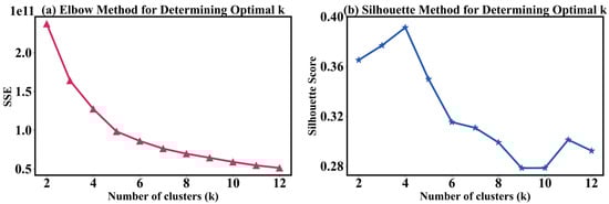
Figure 2.
The best k value chosen by elbow method (a) and silhouette method (b).
- (3)
- K-means clustering procedure
The K-means clustering process includes assignment and update steps:
where is the sample vector, is the centroid of cluster k, and selects the nearest centroid.
where is the number of samples in cluster k and is the updated centroid.
Iterations continue until centroid displacement falls below a threshold. The final analysis identified four circulation regimes representing the dominant large-scale atmospheric patterns associated with wind shear.
2.3. Combination Shear Calculation Method
The combined shear method integrates the radial shear component CRs and the azimuthal shear component CAs to obtain the horizontal shear value Cs of the horizontal wind field under the Plan Position Indicator (PPI) scanning mode of a Doppler wind lidar. The calculation procedure is described as follows [28]:
where v0 denotes the horizontal wind speed at the radial reference point, and vi is the horizontal wind speed at the ith range gate along the same radial direction. r0 and ri represent the distances from the radar center to the reference point and the ith range gate, respectively. ΔR denotes the radial interval, and n is the number of data points within a 200 m range along the radial direction. Similarly, θ0 and θi indicate the azimuth angles of the reference point and the ith gate, respectively, Δθ is the azimuthal interval, and m represents the number of data points within a 20° azimuthal range.
The horizontal shear value Cs is then obtained by vectorially combining CRs and CAs:
This combined shear metric effectively characterizes the horizontal variation in the wind field retrieved from lidar PPI scans, providing a more comprehensive representation of local wind shear.
To facilitate operational interpretation, the severity levels of low-level wind shear used in this study are summarized in Table 1. The classification follows widely adopted shear-intensity criteria, with four categories ranging from light to severe. In accordance with aviation operational practice, a LLWS alert is triggered when the horizontal shear intensity reaches or exceeds 0.068 s−1, corresponding to moderate or stronger wind shear. This threshold ensures that the identified events are meteorologically significant and relevant to flight-safety applications.

Table 1.
Low-level wind shear strength standard of World Meteorological Organization.
2.4. Optimization Method
2.4.1. Optimization Objective
The overall workflow of the optimization method is illustrated in Figure 3. The objective of this study is to construct an optimized wind-shear field Cs*(x,y) by integrating the dynamical contribution of horizontal divergence D(x,y) into the original shear field Cs(x,y).
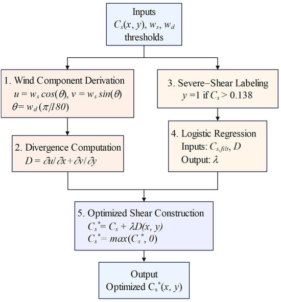
Figure 3.
Flowchart of optimization methods.
The optimized field is defined as a divergence-modulated modification:
where λ is a statistically derived contribution coefficient obtained from logistic regression.
This formulation enhances wind-shear intensity in dynamically active regions (positive divergence) and suppresses noise elsewhere.
2.4.2. Mathematical Procedure
- (1)
- Divergence computation
The wind field divergence D is calculated as
where ws and wd denote the measured wind speed and wind direction (in degrees, clockwise from true north), respectively; u and v are the wind components in the east (x) and north (y) directions.
where u(x,y) and v(x,y) denote the zonal and meridional wind components, respectively.
- (2)
- Divergence-based mask
Then, based on this threshold, a binary mask function M(x,y) is constructed:
The original wind shear values Cs are preserved only within the masked region, while the values outside are set to zero, yielding the divergence-filtered wind shear field:
where Cs(x,y) is the original wind-shear field.
- (3)
- Severe-shear labeling
A binary label is defined using the severe wind shear threshold of 0.138:
- (4)
- Logistic regression
A logistic regression model is then established, with and D as input features:
where β0, β1, β2 are regression coefficients.
The decision boundary of the model is expressed as
The relative contribution of divergence is quantified by introducing the coefficient λ:
This coefficient determines how strongly divergence modulates wind shear.
- (5)
- Construction of the optimized shear field
Accordingly, the optimized wind shear field is formulated according to Equation (9).
To ensure physical consistency, negative values are truncated:
Here, Cs denotes the original wind shear, D the divergence, and λ the relative regression coefficient derived from logistic regression. A positive λ amplifies wind shear in high-divergence regions, while a negative λ reduces it accordingly.
The methods described above provide the basis for analyzing the vertical wind field structure, wind-shear characteristics, circulation patterns, and typical wind-shear processes at ZULS. The results of these analyses are presented in the following section.
3. Results and Discussion
3.1. Wind Field Characteristics
The characteristics of wind field variability significantly influence the take-off and landing of aircraft. It is imperative to analyze the wind field features at Lhasa airport performed under the DBS mode. In the DBS mode, the DWL captured the variation in wind fields at different heights, revealing the vertical distribution characteristics of the wind field over time.
Figure 4 shows the variations in wind speed and direction recorded daily at 00, 06, 12, and 18 LT from 20 May to 30 September 2023. The long-term continuous observations indicated a distinct alternating pattern in wind speed, particularly evident in early June, late August, and mid-September. The significant fluctuations in wind speed during these periods indicated the dynamic characteristics of the wind field. During the daytime, solar radiation heating contributed to the thickening of the boundary layer, increasing wind speed [29]. Conversely, nighttime cooling of the surface led to a reduction in boundary layer thickness and a corresponding decrease in wind speed. Thus, the wind speed in early June exhibited a periodic pattern of increase and decrease, while the variations observed in late August and mid-September further reflected the cyclical nature of this alternating phenomenon. Additionally, the wind speed at ZULS exhibited a strong diurnal variation, with wind speeds reaching 20 m/s on several days. Among these events, the strongest wind, reaching 20 m/s, extended up to approximately 1500 m on the night of June 3 at 18 LT. The minimum wind speed did not exceed 2.5 m/s at 06 LT. In terms of wind direction, vertically, the main airflow direction from the west and north indicated the prevailing wind direction at Lhasa airport during these periods. According to the topographic condition of ZULS (Figure 1), there existed a natural corridor to the north and west, characterized by low-lying areas between mountain ranges, which facilitated air movement. Consequently, the variations in wind direction were closely associated with the local topography.
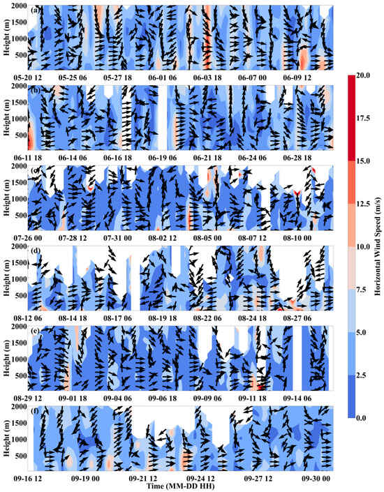
Figure 4.
The hourly average wind field from 00:00, 06:00, 12:00, and 18:00 daily, from 20 May 2023 to 30 September 2023, in the DBS mode. (a) 20 May–10 June 2023; (b) 11 June–30 June 2023; (c) 26 July–11 August 2023; (d) 12 August–28 August 2023; (e) 29 August–15 September 2023; (f) 16 September–30 September 2023. The arrows indicate wind direction (north at 0°, clockwise).
The vertical characteristics of average wind speed and direction (Figure 5) revealed a distinct variation in wind speed over height. It decreased with increasing height until approximately 1000 m, where it began to increase. As shown in Figure 5, wind speed decreases toward the surface below 1000 m, mainly due to surface friction and atmospheric stability. Daytime thermal convection enhances vertical mixing, causing wind speed to increase more rapidly with height, while nocturnal stability leads to notably lower wind speeds near the ground. Local topography and surface roughness further modulate the low-level wind profile. The average wind speed from 20 LT to 02 LT at night (Figure 5b) was overall higher than the average wind speed from 09 LT to 19 LT during the day (Figure 5a). At a height of approximately 100 m, the maximum average wind speed at night could reach 5.2 m/s, while during the day, the maximum wind speed at the same height did not exceed 5 m/s. At a height of 1000 m, the wind speed at night reached 3.9 m/s, whereas during the day, it only reached 3.3 m/s. A similar phenomenon has also been described in [30]. The wind direction exhibited a pattern with westerly winds in the lower layers and northerly winds in the upper layers. During the daytime, the vertical change in wind speed was relatively flat, while the wind direction changed significantly with increasing heights, from southwest to west to northwest and finally to north. In contrast, it revealed more pronounced variations in wind speed over heights at nighttime, characterized by predominantly westerly winds in the lower layers and a distinct concentration of wind direction from the northwest between 600 and 1000 m, while the upper-level winds remained predominantly northerly. The daytime low-level wind direction was more southerly than at night, closely linked to changes in plateau radiation and facilitated by the prominent valleys south of ZULS, which enabled downslope winds from the southern slopes [31,32].
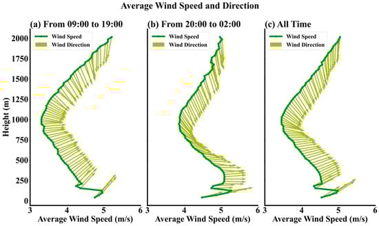
Figure 5.
The average wind speed and wind direction profiles from 09:00 to 19:00 (a), 20:00 to 02:00 (b), and for all hours (c), from 20 May 2023 to 30 September 2023, in the DBS mode.
3.2. Wind Shear Characteristics
To have a clearer understanding of the extent, height, and timing of the susceptibility to low-level wind shear at Lhasa airport during the observation period (summer and autumn), Figure 6 exhibits the temporal and vertical frequency distribution of wind shear. Overall, from 20 May to 30 September 2023 (Figure 6a), wind shear occurred uniformly day and night. From 20 May to 30 June (Figure 6b), wind shear occurred more frequently at night than during the day, mainly in the near-surface layer. At night, surface cooling created a stable boundary layer and low-level jet, all increasing vertical wind shear. During the daytime, wind shear decreased within the mixed layer, where turbulence weakened the wind speed gradient [33]. From 24 July to 30 August (Figure 6c), wind shear distribution remained relatively uniform. Compared to June, the frequency of wind shear during the daytime in September (Figure 6d) significantly increased. Moreover, the frequency of wind shear during the daytime was higher than at night, with daytime occurrences spanning the entire boundary layer. Due to the gradual weakening of solar radiation and reduced surface heating, the boundary of September is shallower compared to June. This results in diminished turbulent mixing and an overall rise in the vertical wind speed gradient, thus elevating wind shear frequencies.
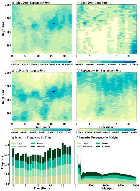
Figure 6.
The occurrence frequency of LLWS in the DBS mode from 20 May 2023 to 30 September 2023 (a), from 20 May to 30 June (b), from 24 July to 30 August (c), and from 1 September to 30 September (d). The stacked bar chart (e) of the LLWS intensity frequency with time, and the stacked area chart (f) of the LLWS intensity frequency with height, both from 20 May 2023 to 30 September 2023, in the DBS mode.
Figure 6e shows significant diurnal variations in wind shear intensity. Severe and extreme wind shear frequencies exhibited notable increases in the evening and nighttime (14–02 LT). Moreover, the cumulative frequency reached its peak at 20 LT, reaching up to 0.2. This phenomenon is related to stable boundary layer formation and nocturnal low-level jets (LLJs). The stability of the nocturnal atmosphere suppressed turbulent mixing, which exacerbated the disparity between surface and elevated wind speeds, further strengthening wind shear. During the daytime (05–13 LT), severe and extreme wind shear frequencies decreased, characterized mainly by light to moderate shear. During this period, the cumulative frequency was approximately 0.15. The vertical gradient of wind speed was more gradual during the day. The mixed layer of the boundary layer was deeper, inhibiting extreme wind shear formation [33]. Figure 6f shows variations in wind shear intensity over heights. A pronounced increase in wind shear frequency existed within the lower 200 m of the atmosphere, primarily due to surface friction and turbulent dynamics, which induced abrupt wind speed fluctuations. At this height, the occurrence frequency of moderate intensity and above was the highest, and a cumulative intensity frequency reached 0.15. At altitudes between 500 and 1500 m, wind shear frequency stabilized, mainly exhibiting light to moderate intensities, with the cumulative intensity frequency of only 0.05. Above 1500 m, wind speed variability decreased, resulting in a gradual attenuation of wind shear intensity, with extreme wind shear occurrences being relatively infrequent. This is related to reduced vertical wind speed variability, which correspondingly diminished both the intensity and frequency of wind shear.
Figure 7a–h show the diurnal and directional variations in low-level wind shear (LLWS) frequency and intensity before and after optimization under the PPI model. The optimized results show a clear decrease in both frequency and intensity. Moderate and stronger events were greatly reduced. The main temporal and directional patterns remained consistent.
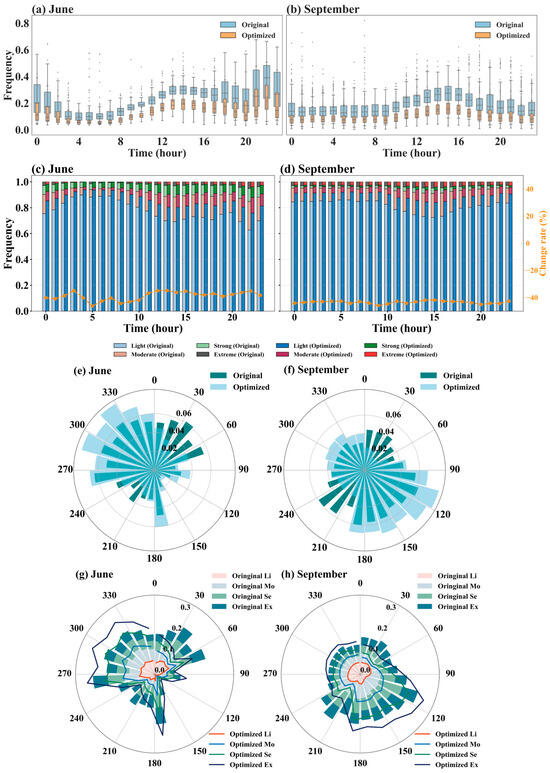
Figure 7.
Under the PPI model, the daily variation box plots of LLWS occurrence frequency in June (a) and September (b), the daily variation stacked bar charts of LLWS intensity frequency in June (c) and September (d), and the wind rose diagrams of LLWS occurrence (e,f) and intensity (g,h) frequency in June and September. The dashed line (right y-axis) indicates the percentage change rate of moderate and stronger LLWS. The overlapping colors represent the overlap between the Oringinal and Optimized detributions.
In June (Figure 7a,c), the optimized LLWS frequency was lower than the original at all hours. The largest reduction appeared in the late afternoon and nighttime (16–24 LT), when LLWS originally peaked. The median frequency dropped by about 30–40%. The interquartile range also became smaller, showing less variability and a more stable wind environment. Strong and extreme LLWS events were greatly reduced, while light shear events dominated after optimization. In September (Figure 7b,d), similar improvements were observed. The diurnal variation was weaker than in June. The optimized LLWS frequency stayed below 0.3 throughout the day. The reduction in moderate and strong intensities was most evident after 12 LT. Compared with June, the optimized September data showed smaller fluctuations and lower uncertainty. This indicates that the optimization stabilized LLWS occurrence in early autumn.
The wind rose diagrams (Figure 7e–h) highlight the directional characteristics and optimization effects. In June, LLWS in the original field mainly came from the north and west. The maximum frequency reached 0.06 in the north-northeast sector. After optimization, the frequencies were significantly lower. The reduction was largest and was reduced by up to 0.03 in the northeast, where strong and extreme LLWS were originally concentrated. The optimized distribution became more uniform, and the overall frequency in all directions decreased by 20–40%. In September, the original LLWS was dominated by southerly and east-southeasterly winds. The frequency peaked around 0.06 in the east-southeast and was lowest (0.03) in the northwest. After optimization, the LLWS frequency and intensity in the southeast declined sharply. The southwest wind shear frequency was reduced by up to 0.04. The wind shear frequency and intensity in the southeast direction are greatly increased. The optimized field displayed weaker directional bias and fewer high-intensity events, though the general seasonal shift from westerly dominance in June to easterly dominance in September remained evident.
3.3. Circulation Characteristics
Cluster analysis was conducted on the 500 hPa geopotential height, 500 hPa winds, and sea level pressure from 20 May to 30 September 2023. Four distinct patterns were identified (Figure 8). In Cluster 1 (Figure 8a), the subtropical high-pressure area remained positioned at 25° N. Lhasa Airport was located on the northern side of the high-pressure ridge. This situation often leads to the convergence of cold and warm air masses, influenced by cold fronts. This may cause significant changes in wind speed and direction. The isobars around ZULS were densely packed, indicating a high-pressure gradient. This suggested that wind speeds were high. Such weather patterns were conducive to the development of wind shear. In the second classification result (Figure 8b), ZULS was situated within a trough of low pressure. Low-pressure troughs were typically associated with upward airflows, which could lead to increased cloud cover and unstable stratification, resulting in the occurrence of wind shear. Figure 8c shows that ZULS was located on the southern edge of the low-pressure trough. It was influenced by the low-pressure system, resulting in upward airflows. The high-pressure gradient indicated that wind speeds remained high. Under the influence of strong winds and unstable stratification, wind shear was likely to occur. In the last classification result (Figure 8d), Lhasa Airport was situated on the edge of a high-pressure system. The isobars were relatively sparse, indicating lower wind speeds, with winds coming from the northeast. The region was under the influence of a high-pressure system, resulting in stable and clear weather. However, due to radiative cooling, the high-pressure system could lead to lower temperatures in the region at night, creating an inversion layer and leading to the occurrence of wind shear.
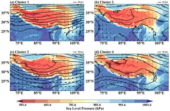
Figure 8.
The four atmospheric circulation types based on K-means clustering analysis from 20 May 2023 to 30 September 2023. The white pentagram represents ZULS.
Additionally, the frequency of wind shear events associated with different circulation types across various months was statistically analyzed, as shown in Figure 9. In May, ZULS was mainly influenced by Cluster 1 and Cluster 3, indicating its position north of the subtropical high and ahead of the low-pressure trough. The proportions of Cluster 1 and Cluster 3 occurring in May were 8% and 11%. In June, Cluster 2 and Cluster 3 circulation patterns occurred more frequently, accounting for 19% and 20%, respectively, with upper-level troughs and their preceding areas significantly influencing the development of wind shear. In August, the circulation patterns were similar to July, with a slight increase in occurrences of Cluster 3. In September, Clusters 1 and 4 were most frequent, accounting for 20% and 19%, with ZULS primarily located north of the subtropical high and under the control of the high-pressure system.
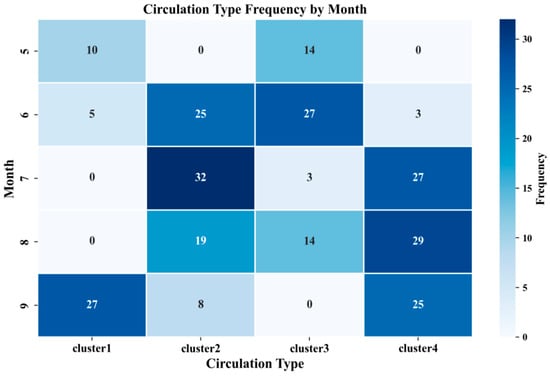
Figure 9.
The heatmap of the occurrence frequency of different atmospheric circulation types for each month.
3.4. Typical Processes in Summer and Fall
This paper selected two typical processes of wind shear, with Figure 10 illustrating the wind shear process on 3 June 2023. In the DBS model, the wind field (Figure 10a) showed that the low-level winds were predominantly westerly, while the upper-level winds were predominantly northerly. The boundary layer thickness exhibits a pattern of first increasing and then decreasing in response to changes in solar radiation. Due to the shallowing of the boundary layer at night, wind speed can increase to 20 m/s at night. In Figure 10b, wind shear of moderate intensity and above occurs throughout the entire boundary layer in the afternoon but is primarily concentrated in the near-surface layer during the nighttime. This study optimized horizontal wind shear under PPI mode, focusing on the afternoon and nighttime. Figure 10c–e show the original horizontal wind fields and wind shear at 14:00 LT on 3 June 2023. Figure 10f–h show the optimized results for the same time. In the original field, moderate and stronger shear appeared in the afternoon. It was mainly concentrated within 3 km in the north. After optimization, shear remained concentrated in the north. The area of moderate and stronger shear increased. Figure 10i–k show the original horizontal wind fields and wind shear at 20:00 LT. Figure 10l–n show the optimized results. At night, moderate and stronger shear was concentrated within 3 km in the west. Compared with the afternoon, wind shear covered a wider area and had higher intensity. After optimization, the false alarm rate in the northwest decreased significantly.
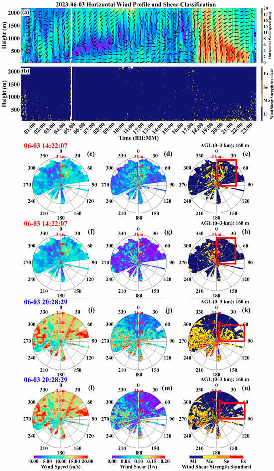
Figure 10.
Under the DBS model: wind speed and direction (a) and LLWS intensity (b) on 3 June 2023. Under the PPI model: wind speed, LLWS values, and intensity at 14:22:07 LT (c–e) and 20:28:29 LT (i–k), with optimized wind speed, LLWS values, and intensity shown in (f–h) and (l–n), respectively. The arrows indicate wind direction (north at 0°, clockwise), and the red boxes highlight regions with pronounced differences in wind shear before and after optimization.
Another typical process was the wind shear event on 3 September 2023 (Figure 11). Compared to June, the boundary layer is shallower in September (Figure 11a,b). This resulted in wind speed in September being lower than in June, with a maximum not exceeding 15 m/s and a higher frequency of moderate and above wind shear intensity during the day. Conversely, nighttime wind shear primarily took place at the top of the shallow stable boundary layer. Figure 11c–e show the original horizontal wind fields and wind shear at 15:00 LT on 3 September 2023. Figure 11f–h show the optimized results for the same time. In the original field, moderate and stronger shear appeared in all directions in the afternoon. It was also located farther from the lidar. After optimization, the scattered shear within 3 km was filtered out. At night, the original field showed moderate and stronger shear with reversed direction. It was mainly concentrated in the southern region. The affected area was within 3 km, with stronger shear intensity. After optimization, the false alarm rate in the southwest decreased significantly. Moderate and stronger shear in the southeast also increased noticeably.
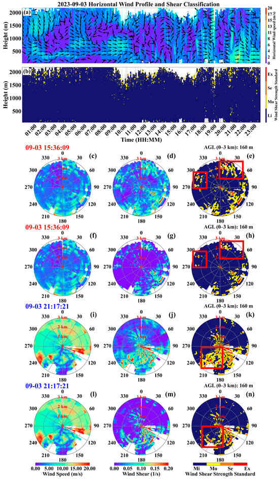
Figure 11.
Under the DBS model: wind speed and direction (a) and LLWS intensity (b) on 3 June 2023. Under the PPI model: wind speed, LLWS values, and intensity at 15:36:09 LT (c–e) and 21:17:21 LT (i–k), with optimized wind speed, LLWS values, and intensity shown in (f–h) and (l–n), respectively. The arrows indicate wind direction (north at 0°, clockwise), and the red boxes highlight regions with pronounced differences in wind shear before and after optimization.
The above results clarify the dominant circulation regimes, the associated wind-shear characteristics, and the performance of the optimized shear field. These findings provide the foundation for the overall conclusions and implications, which are summarized in the following section.
4. Conclusions
This study comprehensively investigated the spatiotemporal characteristics and formation mechanisms of low-level wind shear (LLWS) at Lhasa Gonggar Airport (ZULS) using long-term, high-resolution Doppler Wind Lidar (DWL) observations. In addition, ERA5 reanalysis data were used to analyze the associated large-scale circulation patterns. More importantly, an optimized LLWS detection approach, combining wind field divergence characteristics with logistic regression, was developed and applied to improve detection accuracy and reduce false alarm rates under complex plateau terrain conditions.
The results showed that the prevailing wind field over ZULS was dominated by westerly winds in the lower layers and northerly winds aloft, with a clear diurnal cycle. Wind speeds decreased with height in the near-surface layer and increased again above 1 km, while wind direction exhibited daytime southerly turning influenced by valley winds. LLWS displayed significant seasonal and diurnal variations; in June, shear occurred primarily near the surface during nighttime due to strong radiative cooling and the formation of nocturnal low-level jets; in September, wind shear occurred more frequently throughout the boundary layer during daytime, associated with shallower boundary layers and enhanced vertical wind gradients. The optimization algorithm substantially improved LLWS detection performance. By integrating divergence-based indicators and logistic regression classification, the optimized method effectively reduced the false alarm rate while maintaining the correct identification of true shear events. Compared with the original field, moderate and strong LLWS frequencies decreased by 30–40%, and the spatial distribution of high-intensity events became more concentrated and physically consistent. In June, optimization significantly reduced spurious detections in the northwest and stabilized the temporal variation in LLWS. In September, scattered shear near the airport was successfully filtered out, and the spatial pattern of strong shear became more coherent in the southeast sector. These improvements indicate that the proposed optimization framework can effectively capture real LLWS occurrences and suppress noise-induced false alarms in complex mountainous environments. The circulation analysis revealed that LLWS at ZULS is closely related to four dominant synoptic patterns, including the northern flank of the subtropical high, low-pressure troughs, and high-pressure edges. These large-scale conditions modulate the background wind field and influence the occurrence and intensity of LLWS.
However, some limitations should be noted; the algorithm depends on high-resolution lidar data, which may not be available at all airports, and currently considers only divergence and logistic regression, potentially overlooking small-scale turbulence and other local factors. Future work will focus on extending the algorithm to incorporate additional observational data, such as radar or in situ measurements, and integrating more advanced machine learning techniques to further enhance detection accuracy. Overall, this study not only provides a detailed understanding of LLWS characteristics at a typical plateau airport but also proposes an effective optimization algorithm for LLWS detection. The approach improves the reliability of wind shear warnings, offering valuable technical support for aviation meteorological forecasting, especially in complex terrain regions such as the Qinghai–Tibet Plateau.
Author Contributions
Conceptualization, H.D. and D.Z.; methodology, D.Z.; software, H.D.; validation, H.D., D.Z. and L.D.; formal analysis, H.D.; investigation, J.W.; resources, W.S.; data curation, G.L.; writing—original draft preparation, H.D.; writing—review and editing, H.D. and D.Z.; visualization, H.D. and S.Z.; supervision, T.W.; project administration, Y.L.; funding acquisition, Y.L. All authors have read and agreed to the published version of the manuscript.
Funding
This study was supported by the National Natural Science Foundation of China (42307144), the Second Comprehensive Scientific Research Project on the Tibetan Plateau (2019QZKK0105), and the Fundamental Research Funds for the Central Universities (24CAFUC07001; PHD2023-018).
Institutional Review Board Statement
Not applicable.
Informed Consent Statement
Not applicable.
Data Availability Statement
The data used in this study are available from the corresponding author upon reasonable request. ERA5 reanalysis data are openly available at https://www.ecmwf.int/en/forecasts/datasets/reanalysis-datasets/era5 (accessed on 6 December 2025).
Acknowledgments
The authors thank the European Centre for Medium-Range Weather Forecasts (ECMWF) for providing the ERA5 reanalysis data used in this study.
Conflicts of Interest
The authors declare no conflicts of interest. The funders had no role in the design of the study; in the collection, analyses, or interpretation of data; in the writing of the manuscript, or in the decision to publish the results.
Appendix A
Table A1.
Acronyms used in this study.
Table A1.
Acronyms used in this study.
| Acronym | Meaning |
|---|---|
| DWL | Doppler Wind Lidar |
| PPI | Plan-Position-Indicator scan |
| DBS | Doppler-Beam-Swinging scan |
| LLWS | Low-Level Wind Shear |
| ECMWF/ERA5 | Reanalysis dataset from ECMWF |
Table A2.
Definitions of key symbols used in this study.
Table A2.
Definitions of key symbols used in this study.
| Symbol | Meaning | Unit |
|---|---|---|
| ws | Horizontal wind speed | m·s−1 |
| wd | Wind direction (clockwise from north) | ° |
| u | Zonal (eastward) wind component | m·s−1 |
| v | Meridional (northward) wind component | m·s−1 |
| CRs | Radial shear component | s−1 |
| CAs | Azimuthal shear component | s−1 |
| Cs | Combined horizontal wind shear | s−1 |
| D(x,y) | Horizontal divergence | s−1 |
| Cs* | Optimized wind-shear field | s−1 |
| λ | Divergence contribution coefficient | dimensionless |
| K | Number of clusters in K-means | dimensionless |
| μk | Centroid of cluster k | same as input field |
References
- Ratnasari, Y.; Trilaksono, N.J.; Septiadi, D. Analysis of Low-Level Wind Shear’s (LLWS) Trigger Factors at Soekarno-Hatta International Airport Utilizing Doppler Weather Radar. AIP Conf. Proc. 2024, 2920, 030003. [Google Scholar] [CrossRef]
- Xia, H.; Chen, Y.; Yuan, J.; Su, L.; Yuan, Z.; Huang, S.; Zhao, D. Windshear Detection in Rain Using a 30 km Radius Coherent Doppler Wind Lidar at Mega Airport in Plateau. Remote Sens. 2024, 16, 924. [Google Scholar] [CrossRef]
- ICAO. Manual on Low-Level Wind Shear and Turbulence; International Civil Aviation Organization: Montreal, QC, Canada, 2005. [Google Scholar]
- Ryan, M.; Saputro, A.H.; Sopaheluwakan, A. Review of Low-Level Wind Shear: Detection and Prediction. AIP Conf. Proc. 2023, 2719, 020044. [Google Scholar] [CrossRef]
- Shun, C.M.; Chan, P.W. Applications of an Infrared Doppler Lidar in Detection of Wind Shear. J. Atmos. Ocean. Technol. 2008, 25, 637–655. [Google Scholar] [CrossRef]
- Tsai, C.; Kim, K.; Liou, Y.; Lee, G. Variability in the Microphysical Characteristics Associated with Orographic Airflow in the Mountainous Pyeongchang Region. Mon. Weather Rev. 2025, 153, 691–716. [Google Scholar] [CrossRef]
- Chan, P.W. Case Study of a Special Event of Low-Level Windshear and Turbulence at the Hong Kong International Airport. Atmos. Sci. Lett. 2023, 24, e1143. [Google Scholar] [CrossRef]
- Chan, P.W.; Li, Q.S. Some Observations of Low Level Wind Shear at the Hong Kong International Airport in Association with Tropical Cyclones. Meteorol. Appl. 2020, 27, e1898. [Google Scholar] [CrossRef]
- He, Y.; Cai, J.; Wang, R.; He, X.; Chan, P.; Fu, J. Observation of Downburst Wind Characteristics Using the Doppler Profiler and Near-Ground Measurements. Nat. Hazards 2024, 120, 4829–4851. [Google Scholar] [CrossRef]
- Chan, P.W. Remote-sensing observations of a gust front at Hong Kong International Airport. Weather 2012, 67, 176–181. [Google Scholar] [CrossRef]
- Chan, P.W.; Hon, K.K.; Li, Q.S. Low-Level Windshear Associated with Atmospheric Boundary Layer Jets—Case Studies. Atmósfera 2021, 34, 461–490. [Google Scholar] [CrossRef]
- Chan, P.W.; Hon, K.K.; Li, Q.S. A Comprehensive Study of Terrain-Disrupted Airflow at Hong Kong International Airport—Observations and Numerical Simulations. Weather 2020, 75, 199–206. [Google Scholar] [CrossRef]
- Louis, K.S.; Guan, Y.; Li, L.K.B. RANS Simulations of Terrain-Disrupted Turbulent Airflow at Hong Kong International Airport. Comput. Math. Appl. 2021, 81, 737–758. [Google Scholar] [CrossRef]
- Zhang, H.; Wang, Q.; Wu, S. Low-Level Wind Shear Observation at Beijing Capital International Airport Based on Coherent Doppler Lidar. J. Atmos. Environ. Opt. 2018, 13, 34–41. Available online: http://gk.hfcas.ac.cn/EN/Y2018/V13/I1/34 (accessed on 6 December 2025).
- Zhang, H.; Wu, S.; Wang, Q.; Liu, B.; Yin, B.; Zhai, X. Airport Low-Level Wind Shear Lidar Observation at Beijing Capital International Airport. Infrared Phys. Technol. 2019, 96, 113–122. [Google Scholar] [CrossRef]
- Boilley, A.; Mahfouf, J.F. Wind shear over the Nice Côte d’Azur airport: Case studies. Nat. Hazards Earth Syst. Sci. 2013, 13, 2223–2238. [Google Scholar] [CrossRef]
- Liou, Y.; Yang, P.; Chen, W.; Lee, Y.; Hsu, Y.; Tsai, C.; Lin, P.; Su, B.; Lan, C.; Chen, F.; et al. The Characteristics of Three-Dimensional Wind and Thermodynamic Fields in the Clear-Air Boundary Layer Retrieved by Using Two Scanning Doppler Lidar Observations. Mon. Weather Rev. 2025, 153, 2689–2704. [Google Scholar] [CrossRef]
- França, G.B.; de Almeida, M.V.; Bonnet, S.M.; Albuquerque Neto, F.L. Nowcasting Model of Low Wind Profile Based on Neural Network Using SODAR Data at Guarulhos Airport, Brazil. Int. J. Remote Sens. 2018, 39, 2506–2517. [Google Scholar] [CrossRef]
- Weipert, A.; Kauczok, S.; Hannesen, R.; Ernsdorf, T.; Stiller, B. Wind Shear Detection Using Radar and Lidar at Frankfurt and Munich Airports. In Proceedings of the 8th European Conference on Radar in Meteorology and Hydrology, Garmisch-Partenkirchen, Germany, 1–5 September 2014; pp. 1–5. Available online: http://www.pa.op.dlr.de/erad2014/programme/ExtendedAbstracts/058_Weipert.pdf (accessed on 6 December 2025).
- Zhao, S.; Shan, Y. Study of the Algorithm for Wind Shear Detection with LiDAR Based on Shear Intensity Factor. Algorithms 2022, 15, 133. [Google Scholar] [CrossRef]
- Ryan, M.; Saputro, A.H.; Sopaheluwakan, A.H. Intelligent Low-Level Wind Shear Alert Prediction System Based on Anemometer Sensor Network and Temporal Convolutional Network (TCN). Geogr. Tech. 2022, 17, 92–103. [Google Scholar] [CrossRef]
- Stratton, D.A.; Stengel, R.F. Robust Kalman Filter Design for Predictive Wind Shear Detection. IEEE Trans. Aerosp. Electron. Syst. 1993, 29, 1185–1194. [Google Scholar] [CrossRef]
- Weber, M.E.; Stone, M.L. Low Altitude Wind Shear Detection Using Airport Surveillance Radars. In Proceedings of the 1994 IEEE National Radar Conference, Atlanta, GA, USA, 29–31 March 1994; pp. 52–57. [Google Scholar] [CrossRef]
- Lin, C.; Zhang, K.; Chen, X.; Liang, S.; Wu, J.; Zhang, W. Overview of Low-Level Wind Shear Characteristics over Chinese Mainland. Atmosphere 2021, 12, 628. [Google Scholar] [CrossRef]
- Liu, Z.; Barlow, J.F.; Chan, P.W.; Fung, J.C.H.; Li, Y.; Ren, C.; Mak, H.W.L.; Ng, E. A Review of Progress and Applications of Pulsed Doppler Wind LiDARs. Remote Sens. 2019, 11, 2522. [Google Scholar] [CrossRef]
- Graßl, S.; Ritter, C.; Schulz, A. The Nature of the Ny-Alesund Wind Field Analysed by High-Resolution Windlidar Data. Remote Sens. 2022, 14, 3771. [Google Scholar] [CrossRef]
- Jin, H.; Chen, X.; Wu, P.; Song, C.; Xia, W. Evaluation of Spatial-Temporal Distribution of Precipitation in Mainland China by Statistic and Clustering Methods. Atmos. Res. 2021, 262, 105772. [Google Scholar] [CrossRef]
- Fan, Q.; Zheng, J.-F.; Zhou, D.-F.; Zhu, K.-Y.; Zhang, J.; Tong, W.-H.; Luo, X. Research on Airport Low-Level Wind Shear Identification Algorithm Based on Laser Wind Radar. J. Infrared Millim. Waves 2020, 39, 462–472. [Google Scholar]
- Smith, D.K.E.; Renfrew, I.A.; Price, J.D.; Dorling, S.R. Numerical Modelling of the Evolution of the Boundary Layer during a Radiation Fog Event. Weather 2018, 73, 310–316. [Google Scholar] [CrossRef]
- Zheng, J.; Liu, Y.; Peng, T.; Wan, X.; Huang, X.; Wang, Y.; Che, Y.; Xu, D. Investigating Wind Characteristics and Temporal Variations in the Lower Troposphere over the Northeastern Qinghai–Tibet Plateau Using a Doppler LiDAR. Remote Sens. 2024, 16, 1840. [Google Scholar] [CrossRef]
- Huang, X.; Zheng, J.; Shao, A.; Xu, D.; Tian, W.; Li, J. Study of Low-Level Wind Shear at a Qinghai-Tibetan Plateau Airport. Atmos. Res. 2024, 311, 107680. [Google Scholar] [CrossRef]
- Malek, A. Empirical Analysis of Processes Affecting Drainage Flows and Inversions in a Forested Mountain Landscape. Ph.D. Thesis, Oregon State University, Corvallis, OR, USA. Available online: https://ir.library.oregonstate.edu/concern/graduate_thesis_or_dissertations/bc386q546 (accessed on 6 December 2025).
- Halios, C.H.; Barlow, J.F. Observations of the Morning Development of the Urban Boundary Layer over London, UK, Taken during the ACTUAL Project. Bound.-Layer Meteorol. 2018, 166, 395–422. [Google Scholar] [CrossRef]
Disclaimer/Publisher’s Note: The statements, opinions and data contained in all publications are solely those of the individual author(s) and contributor(s) and not of MDPI and/or the editor(s). MDPI and/or the editor(s) disclaim responsibility for any injury to people or property resulting from any ideas, methods, instructions or products referred to in the content. |
© 2025 by the authors. Licensee MDPI, Basel, Switzerland. This article is an open access article distributed under the terms and conditions of the Creative Commons Attribution (CC BY) license.