Abstract
Vegetation phenology, particularly the start of the growing season (SOS) date, is a key indicator of the climate sensitivity of ecosystems, yet its accurate prediction remains challenging. This study investigates the SOS of Hungarian grasslands between 2000 and 2023 using MODIS NDVI data, testing ten process-based models of varying complexity. Model parameters were optimized with the differential evolution algorithm under three calibration strategies: generic (GEN, aiming for a single model setting for the country), grassland-type (GEN GRASS, where grasslands are first categorized and then a type-specific parameterization is sought), and pixel-level (PIX, where model parameterization is performed for each pixel separately). The models with the lowest RMSE values were AGSI and AHSGSI (driven by temperature, vapor pressure deficit, and photoperiod) under PIX (RMSE = 3.3 days), AGSIwSW (driven by temperature, soil water content, and photoperiod) under GEN and GEN GRASS (RMSE = 7.6 and 6.3 days, respectively), and MGDDwPP (driven by temperature and photoperiod) under GEN (RMSE = 7.6 days). Considering the Akaike Information Criteria, the simplest GDD model (driven by temperature only) was the proposed one under PIX, while MGDDwPP was identified as the best model both in GEN and GEN GRASS. Residual analysis revealed relatively strong co-variation between model errors and some basic climate anomalies (most of all spring temperature and soil water content), enabling statistical corrections that reduced bias close to zero across all models. Integrating local climate and soil information into phenology models enhances their accuracy for grassland SOS estimation in Central Europe.
1. Introduction
Plant phenology is a major indicator of the ongoing, large-scale environmental changes that affect many terrestrial properties and processes, including albedo, surface roughness, carbon balance, evapotranspiration, surface energy balance, greenhouse gas emission, and others [1,2,3]. Phenology observations span from individual plants [4,5,6,7] to regional and global patterns [8,9,10,11,12], covering markedly different spatial scales. In the mid-latitudes seasonality triggers spectacular changes in the foliage development of the different biomes that attracted scientific interest even several hundred years ago [13,14]. Since then, numerous studies have focused on the phenology of forests, grasslands, and other biomes [15]. Yet, despite the interest and recent advances, plant phenology is still not well understood due to the complexity of the environmental factors, studied spatial scales, and lack of process understanding [16,17,18]. This is especially true for grasslands due to the diversity of herbaceous vegetation. For example, White et al. (1997) found that the interannual variability of the phenological cycle of grasslands is more variable than those of forests, making them sensitive indicators of climate fluctuations and extremes [19]. Given the important role of grasslands and semi-arid ecosystems in the interannual variability of the land surface carbon sink [20], understanding their phenology is of great importance.
Biogeochemical and earth system models (ESMs) all quantify the phenology events of ecosystems, including the start of the growing season (SOS) and cessation of foliage cover (end of season), since almost all simulated processes interact with phenology. The misrepresentation of phenology is a major issue in these models that need improvement. For example, Wu et al. (2021) demonstrated that early growing season anomalies largely determine the annual vegetation–climate coupling; thus, accurate SOS estimation is essential for model realism [21]. As shown by Mo et al. (2023), globally applicable models often fail to capture ecosystem-specific dynamics, which is particularly problematic in grasslands [22,23]. Given the abundance of phenology models, the selection and spatial generalization of these models need special attention and improvement.
The present study focuses on the SOS date estimation of grasslands. Grassland phenology studies are typically characterized by the lack of rich in situ observations and a standard definition of grassland SOS. Most of the grassland-related studies rely on remote sensing data that provides an alternative way to quantify SOS in relatively larger spatial scales. Remote sensing-based studies use custom definitions to detect SOS [24], which sometimes makes it hard to compare the models and their performance. Remote sensing-based SOS detection relies on vegetation indices (VIs). However, given the diversity of the remote sensing-based VIs, there are many options that could be possibly used. For example, the recently published High-Resolution Vegetation Phenology and Productivity (HR-VPP) dataset (Copernicus Land Monitoring Service, 2017–present) uses the VPP index to estimate (among others) SOS. Balzarolo et al. (2016) [25] studied different VIs and found that the results of the NDVI-based SOS detection showed the strongest agreement with the SOS derived from eddy covariance measurements based on net ecosystem exchange of carbon dioxide (NEE) when considering all plant functional types. In this study we followed this approach also since many previous studies successfully applied NDVI for Central Europe, and quality-controlled and processed NDVI was already available from earlier works [25,26].
The target area is Hungary (located in Central Europe), which is characterized by a relatively large diversity of grasslands and diverse pedo-climatic conditions that span from dry sandy grasslands with very low productivity to humid grasslands in Western Hungary characterized by large NPP and yield [27]. Grassland-related studies are relatively rare in the region, with some notable exceptions. Kroël-Dulay et al. (2015) [28] and Orbán et al. (2023) [29] examined Hungarian and Central European grasslands, documenting drought-driven dominance shifts. Other studies documented the eddy covariance-based carbon balance of Hungarian grasslands, highlighting their climate sensitivity [28,29,30,31,32]. In any case, there is a growing need to characterize Central European grasslands, especially their phenological cycle, due to the ongoing environmental changes and extreme events. Studying SOS of Hungarian grasslands is a relevant added value, as it is largely missing from the literature.
The overarching aim of this study was to improve our understanding of the drivers and model-based estimation of the SOS date in Hungarian grasslands, with a particular focus on climatic sensitivity. To achieve this, we addressed the following main goals: (1) development of a custom SOS date dataset using a refined, satellite-based method specifically for grassland ecosystems, enabling a more accurate representation of the unique characteristics of Hungarian grassland types; (2) testing and comparing ten process-based phenology models with different levels of complexity and environmental drivers to estimate SOS; (3) assessing the effect of model calibration strategy—spanning from generic to grassland-type and pixel-level approaches—on the estimation of the SOS date; (4) identifying possible drivers of model errors through residual analysis with selected climatic anomalies.
The study can contribute to the improvement of phenology models in a spatially explicit context.
2. Materials and Methods
2.1. Target Area and Grassland Categorization
Hungary, situated in Central Europe, serves as the target area of the present research. The detailed Ecosystem Map of Hungary, developed within the so-called NÖSZTÉP project [33], was used to select these grassland categories. This ecosystem map (hereafter referred to as the NÖSZTÉP dataset) integrates multiple national databases and satellite remote sensing data, such as Sentinel imagery from the period 2015–2017. The dataset distinguishes 56 ecosystem types, including 7 grassland types, with a spatial resolution of 20 m. The analysis focuses on 4 different grassland types that represent the majority of Hungarian grasslands (following the official NÖSZTÉP nomenclature): Open sand steppes, Closed sand steppes, Salt steppes and meadows (grasslands affected by salinization included), and Closed grasslands in hills and mountains or on cohesive soil, together covering approximately 80–85% of the national grassland area [27]; Figure 1). For this study, the NÖSZTÉP dataset was initially aggregated to the grid of the used QKM (quarter km by quarter km) MODIS data with a nominal 250 m × 250 m spatial resolution discussed below.
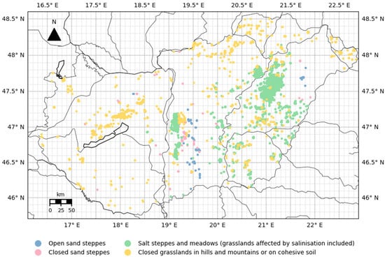
Figure 1.
Spatial distribution of selected grassland types in Hungary based on NÖSZTÉP. Colored dots represent grassland pixels at 250 m spatial resolution. The spatial resolution of the used meteorological database is also indicated (Gaussian grid at 0.1° × 0.1° resolution). Note that the grassland pixels are enlarged for better visualization.
As a first step, grass-covered pixels suitable for further analysis were selected. A given QKM pixel was included in the database if at least 90% of its area and at least 70% of its neighbors were covered by grassland of the same category. The processed grassland database contains ~12,000 QKM pixels (see Table 1 and Figure 1).

Table 1.
Grassland types (left), the proportion (%) of utilized 250 m × 250 m resolution pixels relative to the total number of grassland pixels (right).
2.2. SOS Metrics
2.2.1. Vegetation Index Dataset
Normalized Difference Vegetation Index (NDVI) derived from the official MOD09Q1 (Collection 6.1; [34]) data of the MODerate resolution Imaging Spectroradiometer (MODIS) with a spatial resolution of 250 m × 250 m (QKM) was used to analyze grassland dynamics across the study area from 2000 to 2023. NDVI is a widely used vegetation index based on the difference of the reflectances in the visible and near-infrared spectral bands [35,36]. Preprocessing of the dataset included quality filtering, in which only the highest-quality data were retained following the methodology of Kern et al. (2020) [9]. Missing values were filled using linear interpolation, based on the actual acquisition dates.
To reduce noise while preserving key patterns and trends in the NDVI time series, we applied a moving average smoothing technique. This approach allowed for the smoothing of local fluctuations in the data without compromising the underlying vegetation dynamics. The moving average method (with a 15-day window) that was used is a flexible and robust smoothing method that does not require intensive parameter estimation, unlike logistic function fitting, where parameter values often lack ecological or biological interpretability [37].
2.2.2. Start of Season Date Estimation Method
The start of the season was determined using the commonly applied G50 method [19,38,39]. To estimate the onset of the growing season, was calculated, which represents the relative progression of vegetation development regardless of vegetation type:
For this calculation two key points were identified: , that is the minimum NDVI value prior to day of year (DOY) 90, while is the maximum NDVI value during the period from DOY 90 to DOY 213. In the literature and are defined as the minimum and the maximum of the annual NDVI cycle [38]; however, in grassland systems, a secondary autumn NDVI peak can occur in some years, which may significantly shift the and, consequently, the SOS estimate. Therefore, accurately identifying within the appropriate time window is critical for modeling the vegetation cycle and correctly timing spring phenological events. SOS was defined as the date when the reached 50% of the seasonal NDVI amplitude. The method is illustrated in Figure 2.
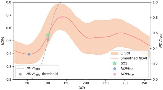
Figure 2.
Illustration of the G50 method to determine the start of the growing season (SOS) date. The red line shows the smoothed average NDVI curve for Hungarian grasslands obtained via moving average, while the shaded orange area indicates the standard deviation around the mean NDVI curve. The dark grey dashed line represents the (see Equation (1); right y-axis), and the grey dot indicates the NDVI threshold (0.5). and are marked in blue and pink, respectively, and the green star represents the point on the NDVI curve where the reaches the threshold; the corresponding projection on the x-axis represents the estimated SOS. Note that although an average NDVI curve representing the 23-year mean (2000–2023) is displayed here for clarity, the SOS is computed on a pixel-by-pixel basis in the analysis.
2.3. Driving Datasets
The models were primarily driven by the FORESEE-HUN v1.2 climate database [40] containing observation-based meteorological data for 2000–2023. FORESEE disseminates the seamless combination of observation-based interpolated data and climate projections. The database provides daily data at a spatial resolution of 0.1° × 0.1°, including daily minimum (Tmin, [°C]) and maximum temperatures (Tmax, [°C]), from which average temperatures (Tavg, [°C]) were calculated as the mean of Tmin and Tmax. In addition, the dataset contains daylight vapor pressure deficit (VPD, [Pa]) and day length (also referred to as photoperiod, PP [s]).
As a product of the European Space Agency’s (ESA) Soil Moisture Essential Climate Variable (ECV) Climate Change Initiative (CCI) project, the ESA CCI Soil Moisture dataset, more precisely the COMBINED v09.1 dataset, provides a globally consistent soil water content (SWC) time series derived from multiple satellite sources. The dataset spans the period from 1 November 1978 to 31 December 2023, offering daily estimations of volumetric soil water content at a spatial resolution of 0.25° × 0.25°, representing the top 5 cm of the soil [41,42]. While ESA CCI Soil Moisture is not an in situ dataset, it is derived from both active and passive microwave satellite observations and is thus considered observation-driven. The dataset includes quality flags (e.g., frozen soil, dense vegetation, radio frequency interference) but does not contain interpolated values. Although an interpolated version became available in January 2025 (ESA CCI SM GAPFILLED [43,44]), we utilized the COMBINED dataset, which includes only actual satellite observations. This choice was motivated by technical considerations, as the official Python package esa_cci_sm (version 0.5.0; https://esa-cci-sm.readthedocs.io/en/latest/, accessed on 19 March 2025)—which provides tools to convert the standard ESA CCI SM NetCDF-4 image files into continuous time series—does not yet support the GAPFILLED product. To address missing values while preserving the integrity of the original data, nearest neighbor interpolation was applied. This method maintains local extremes more effectively, which can be crucial for interpreting modeling uncertainties. The applicability of ESA CCI soil moisture data (v5.2 and v6.1) was assessed at the European scale by Pataki et al. (2025) [44], who demonstrated its suitability for large-scale analyses while noting that performance can vary with climatic and topographic conditions.
2.4. Phenology Models
A large number of mathematical models of varying complexity are available in the scientific literature to quantify specific phenological events [15,45,46,47,48,49,50]. Meteorological variables play a central role in phenological models [15,19,49,51], serving as the main driving data at a given point. In many cases the focus is on the start of the active growing season in mid- and high latitudes [16,52]. Based on the literature review, we selected 10 SOS models that represent different complexity and data requirements. We selected models that span from the simplest and most popular one (using heat sum) to more complex models that use chilling requirements, soil water content, and photoperiod. Detailed information on the models is provided in the Supplementary Materials. Table 2 summarizes the models used in this study, including their abbreviations, number of adjustable parameters, and the driving meteorological variables.
Table 2.
List of the ten SOS models and the ensemble applied in this study with their abbreviations, number of adjustable parameters, and the used input meteorological variables. Detailed information about the models is available in the Supplementary Materials.
The models can be grouped according to their main driving mechanisms. The simpler thermal-based formulations, such as GDD and MGDD models, rely on Tavg, with the latter introducing an additional parameter to increase flexibility. The MGDDwPP model extends this approach by incorporating photoperiod, thereby accounting for the influence of daylength on phenological development. The SEQ and PAR models are temperature-driven formulations with four adjustable parameters, differing mainly in how thermal, chilling accumulation, and threshold processes are combined. In contrast, the GSI-type models (GSI, HSGSI, AGSI, AGSIwSW, and AHSGSI) represent more complex formulations that integrate multiple meteorological drivers, including minimum temperature Tmin, VPD, PP, and in some cases Tavg (HSGSI and AHSGSI) and SWC (AGSIwSW). These models aim to capture the joint effects of thermal, atmospheric, and hydrological constraints on early vegetation activity. More advanced formulations, such as the accumulated GSI models (AGSI, AHSGSI, and AGSIwSW), further incorporate temporal accumulation of these bioclimatic indices, thereby capturing both the intensity and persistence of favorable conditions leading up to SOS. Finally, an ensemble (ENS) model was constructed by averaging the results of all individual models to obtain a more robust and generalized SOS estimate.
2.5. Optimization of the SOS Models
All phenology models contain adjustable parameters that can be set by the user for application (for the adjustable parameters, see Supplementary Materials Tables S8 and S9 and Figures S8–S17). Since these are mainly empirical parameters, setting them based on direct measurements is not possible; however, their adjustment has a significant effect on the model performance, which calls for a mathematical solution.
In general, we assume that an optimal parameter combination exists that minimizes the model error. The model error can be defined in multiple ways, but two of the most common approaches are (i) using a general misfit function or (ii) building a probabilistic model of the error. In this study, the former approach was applied, with the Mean Absolute Error (MAE) chosen as the misfit function. MAE was selected as it is simple to interpret, and no prior knowledge of the parameter distributions was present. Because not all models (e.g., GSI) were differentiable, a derivative-free method was required.
We used the evolutionary algorithms for model optimization [53]. Evolutionary algorithms are mimicking natural selection, and it is known to be an effective optimization tool when the number of parameters is not too high [54,55]. These algorithms are flexible enough to be applied across a wide range of problems, though this flexibility comes at the cost of computational efficiency. To address this limitation for models with continuous parameters, the Differential Evolution algorithm was developed [56], simplifying important settings of the algorithm (mutation and crossover steps) while maintaining robustness. This algorithm was employed in the present study.
The optimization was performed using the Scipy Python (version 1.15.0) library [57]. The parameters of the differential_evolution function were kept at their default settings, while the search bounds are set by expert knowledge (i.e., based on literature search and preliminary consistency check) and are provided in the Supplementary Materials (Tables S8 and S9).
For the calibration, the remote sensing-based SOS data were split into two subsets: from the 24-year dataset, 19 years were allocated for training, while the other years were selected for testing (i.e., independent validation). The division was made with an 80–20% split, where the criterion for selecting the test years was to ensure that the spatial averages of SOS were as similar as possible in both subsets. The test years were 2001, 2008, 2012, 2015, and 2022.
The models were optimized with three different approaches. In the first case, a generic parameterization was constructed across the entire country, where one single parameter set was sought for all grasslands. This kind of optimization is useful for biogeochemical models, crop models, or generic phenology models at larger spatial scales. This approach is referred to as GEN. Using the second approach, the models were optimized separately for each grassland type, as it is supposed to provide more detailed parameterization, resulting in the number of model parameter sets matching the number of four distinct grassland types (Table 1). GEN GRASS identifies the parameters that were set using this method. In the third approach, an individual calibration was performed for each grassland QKM pixel, meaning that the number of parameter sets corresponded to the number of QKM pixels. This approach is referred to as PIX hereafter.
2.6. Data Preparation and Statistical Analysis
The constructed SOS observation dataset spans the period 2000–2023 on 250 m × 250 m spatial grid. In comparison, the FORESEE dataset offers daily climate data at a spatial resolution of 0.1° × 0.1°, while ESA CCI dataset is available at a spatial resolution of 0.25° × 0.25°. The phenological models were executed on the QKM grid, consisting of 12,076 pixels in total. For each QKM pixel, the corresponding driving data were extracted from the nearest point on the original resolution grid.
The performance of the phenology models is quantified by using different statistical measures. Root-mean-square error (RMSE), bias, and R2 (for definitions, see e.g., [58]) were computed for each calibrated model (Table 2). These statistics represent pixel-level performance based on the independent validation years (see Section 2.5), meaning that the time dimension is ignored here, but the overall ability of the models’ spatial SOS patterns is quantified. We also quantified the interannual variability of the models (see Section 3.2). The performance of the models using the three calibration approaches is also visualized in the form of x-y scatterplots.
In addition to traditional error metrics (RMSE, bias, and R2), we also calculated the Akaike Information Criterion (AIC) for each calibration approach. AIC provides a measure of model performance that accounts not only for goodness of fit but also for model complexity, thereby enabling a more balanced comparison across models of different structures [59]. For a model with parameters and log-likelihood (details are available in the Supplementary Materials, Equation (S17), AIC is defined as:
where is a normal likelihood. k is determined by the structure of each phenology model, which is documented in the Supplementary Materials, where all model formulations and calibrated parameters are presented. For GEN calibration, k corresponds to the number of parameters estimated for a given model. For the GEN GRASS calibration, this number is multiplied by the four grassland types considered. For the PIX calibration, k is multiplied by the number of pixels (12,076), reflecting pixel-wise parameter estimation. AIC is calculated for the test years set.
All analyses were performed using Python 3.10.0 (available at https://www.python.org, accessed on 19 March 2025) programming environment.
2.7. Residual Analysis and Construction of Corrected Models
An attempt was made to identify the possible causes of the model errors. For this purpose, the correlations between model residuals (i.e., the difference between model-predicted and remote-sensing-based SOS expressed by DOY, where positive residual means that the model predicted delayed SOS relative to the observations, while negative residual indicates that the modeled SOS date was earlier than in reality) and anomalies of Tmin, Tmax, VPD, and SWC were examined, as they are associated with plant growth by some direct mechanism. The analysis was completed at a monthly time scale for the environmental data. Potentially influencing months were selected based on the timing of the modeled SOS (assuming short-term effect on SOS). The selected months included the January–May time period of the current year and November to December from the previous year. For the spring months, only those site-year combinations were included where the SOS occurred afterward, ensuring that potential spring month anomalies could still influence the SOS date timing.
Residual analysis was performed using the complete, 24-year-long time series within a repeated k-fold cross-validation. Spatial pixels were randomly partitioned into five folds, and Pearson correlation coefficients between meteorological anomalies and model residuals were computed separately for each fold. For each fold and repetition, pixel-wise monthly anomalies were computed by subtracting the long-term climatological mean (averaged over 24 years) from the corresponding monthly mean values for each meteorological variable. In each iteration, correlations were evaluated only on the held-out pixel subset, while the remaining pixels were excluded from that particular correlation estimate. This procedure ensured that the strength and significance of the residual meteorology relationships were assessed on mutually independent subsets of the spatial domain. The resulting correlation estimates were averaged across all folds and repetitions to obtain robust mean correlation values. Statistical significance was assessed using Bonferroni-corrected p-values.
For further investigation and possible adjustment of the modeled SOS, a multiple linear regression framework was applied. Only those meteorological variables and months that showed statistically significant correlations in the cross-validated analysis were retained for the correction procedure. Monthly anomalies were used as predictors in a least-squares regression to model the residuals of the original simulations. The regression was performed over the full spatial and temporal domain, with the resulting coefficients representing the sensitivity of model errors to interannual variability in each meteorological driver. The fitted relationship was subsequently used to correct the model outputs, thereby reducing model error associated with climate anomalies. Error metrics were calculated to check the possible improvement in the model performance.
3. Results
3.1. Remote Sensing-Based Reference SOS
The SOS date shows substantial interannual variability across the four investigated grassland types in Hungary during 2000–2023, with detailed statistics provided in Supplementary Figure S1. The range of the observed SOS is quite large, spanning from 40 to 160 days across all grassland types, indicating high variability in the SOS. Among the vegetation types, the average SOS is around DOY 116 (26th April) for Open sand steppes, DOY 114 (24 April) for Closed sand steppes, DOY 101 (11 April) for Salt steppes and meadows (grasslands affected by salinization included), and DOY 110 (20 April) for Closed grasslands in hills and mountains or on cohesive soil. Median values do not differ much from the average. Salt steppes and meadows (grasslands affected by salinization included) exhibit the earliest SOS, with a narrow interquartile range, indicating relatively low variability between years. In contrast, Open sand steppes have the latest and most variable SOS, with a wider spread of values across years. The SOS date distributions of Closed sand steppes and Closed grasslands in hills and mountains or on cohesive soil are less skewed, with intermediate medians and variability.
The lower tail of the SOS date distribution shows greater spread, with differences of up to 33 days between the minimum and 1st percentile (P1) values (e.g., 40 to 70 days in Open sand steppes), indicating extreme early cases. In contrast, the upper tail is tightly clustered, with differences between P95 and the maximum generally ≤18 days and often only 1–3 days between P99 and the maximum, suggesting that late extremes are rare.
The aggregated statistics for all grasslands yield an average SOS of 103 days, with P5 and P95 values of DOY 84 and 123, respectively, likely reflecting the diversity in environmental and ecological conditions across grassland types. For the detailed basic statistics, see Table S1 in the Supplementary Materials.
Differences among grassland types were examined using a one-way Kruskal–Wallis test, which revealed a significant overall effect of grassland type on SOS date. Post-hoc pairwise comparisons with Dunn’s test (Bonferroni-corrected) identified significant differences between Open sand steppes and Closed grasslands in hills and mountains or on cohesive soil, and between Salt steppes and meadows (grasslands affected by salinization included) and Closed grasslands in hills and mountains or on cohesive soil. No other pairwise comparisons were statistically significant. The p-values are available in Table S5 in the Supplementary Materials.
Figure 3 shows the interannual variability of SOS for Hungary using the categorization that we apply. According to Figure 3, the four categories typically behaved similarly in one particular year with a few exceptions (e.g., 2007 and 2020). The interquartile range is generally narrow, typically 10–15 days, but can expand substantially (reaching its maximum, that is, 79.2 days for Open sand steppes in 2020). Trend analysis revealed that only 9.6% of the pixels showed a significant (p < 0.05) SOS trend of +1 day/decade (delayed SOS). This suggests that climate change did not cause a remarkable shift in SOS dates in the past 24 years, which is somewhat surprising. However, visual inspection suggests certain temporal tendencies; for instance, from 2008 to 2013 there is a gradual delay in the SOS values, similarly to the period between 2001 and 2006. The years 2007 and 2020 stand out as extremes in the sense that the difference between the categories is more emphasized, plus the SOS varies in a wide range in 2020 and partly in 2007 for some grassland types. Nevertheless, a more detailed investigation is beyond the scope of the present study; further investigations are left for future research.
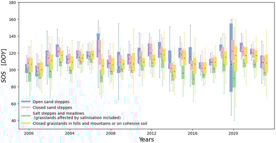
Figure 3.
Interannual variability of SOS across grassland types during the study period, calculated as the mean SOS for the whole country in a particular year. The box height represents the spread of the middle 50% of the observations (from the 25th to the 75th percentile), while the black line inside the box marks the median. The whiskers extend to the most extreme values within 1.5 times the interquartile range. Different box colors correspond to different grassland types.
3.2. Performance of the Models
Figure 4 shows the relationship between the observed and simulated SOS for the MGDDwPP model based on the different calibration approaches. MGDDwPP is presented here as an example, as it is representative of the majority of the other models. Supplementary Materials shows similar graphs for all other models and for the ensemble approach as well (Figures S2–S4). Comparison of the plots shows that there is no superior model to simulate SOS among the tested models. The ensemble is not different from the other process-based models, which is not surprising considering the structural similarities of the applied models leading to shared biases.
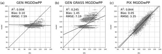
Figure 4.
Pixel-level performance of the MGDDwPP model, under the three calibration strategies: (a) generic calibration (marked as GEN), (b) grassland-type specific calibration (GEN GRASS), and (c) pixel-level calibration (PIX). The dashed line indicates the 1:1 relationship between observed and modeled values, while the solid line shows the result of the linear regression. Accompanying statistics (R2, bias, and RMSE) were computed over the independent test years.
Figure 5 visualizes the relationship between the area averages for the observed and simulated SOS based on the selected representative MGDDwPP model. The plot demonstrates that the model captures the interannual variability of SOS in all three cases relatively well. Clearly, the pixel-level errors compensate each other, and this leads to a robust estimation for the country mean and its variability.
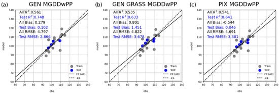
Figure 5.
Relationship between the area-averaged observed and simulated SOS for the MGDDwPP model under three calibration schemes: (a) generic calibration, (b) grassland-type specific calibration, and (c) pixel-level calibration. Gray points represent training data, while blue points indicate validation years. The dashed line denotes the 1:1 relationship, while the solid line is the result of the linear regression. Statistical metrics (R2, bias, and RMSE) are reported both for the full dataset (including training and validation years), with test-year values highlighted in blue.
The statistical evaluation of all calibration strategies and models is summarized in Table 3. According to the table, RMSE varies between 7.6 and 10.6 days for GEN. Under GEN GRASS, RMSE is the highest for MGDD (13.6 days) and HSGSI (13.7 days), indicating that those are the least reliable models overall. PIX calibration yielded the lowest RMSE values across nearly all models, ranging from 3–4 days (AGSI, MGDDwPP, and SEQ) to 6.5 days (GSI and HSGSI).
Table 3.
RMSE, bias, and R2 for each phenology model under three calibration schemes (GEN, GEN GRASS, and PIX). The statistics represent pixel-level performance, quantifying the spatial correspondence of SOS patterns across models computed from independent validation years. The lowest RMSE values are highlighted with bold underlined letters per modeling strategy.
Within the GEN calibration, the MGDDwPP and GDD models were associated with the most favorable bias values (i.e., close to zero). For the GEN GRASS calibration, AGSI, SEQ, and PAR were associated with the lowest bias. Under the PIX calibration, MGDDwPP, SEQ, and PAR yielded the most favorable results, while AGSI also showed notably low bias.
Table 3 presents the R2 values as well for each model across the different calibration approaches. Under the GEN calibration, nearly all models were associated with very low R2. In the GEN GRASS calibration, AGSIwSW continued to demonstrate the best performance. In contrast, HSGSI and AHSGSI perform poorly under this calibration method. The PIX calibration approach yields substantially higher R2 values overall, particularly for MGDDwPP, AHSGSI, and AGSI.
The ensemble approach did not turn out to be superior. Its performance was average, with no indication of any benefit that could be exploited. Scatterplots for all remaining models, along with the ensemble approach, are provided in the Supplementary Materials (Figures S5–S7). The calibrated parameters are also available in the Supplementary Materials (Figures S8–S17).
As the summary of the statistical evaluation, we ranked the models according to RMSE, which is the standard and most frequently used metric for SOS model quantification in the literature (e.g., [22]). In this sense MGDDwPP and AGSIwSW are preferred under GEN and AGSIwSW under GEN GRASS, while AHSGSI and AGSI under PIX.
3.3. AIC
Akaike Information Criterion (AIC) values were calculated separately for GEN, GEN GRASS, and PIX approaches, using all pixels and test years. The resulting AIC values are summarized in Table 4.
Table 4.
AIC values of models calibrated using GEN, GEN GRASS, and PIX approaches. Models are listed in ascending order based on their AIC values.
Considering AIC, the top three models were consistently those that are heat sum-based, with the exception of the GEN calibration, where AHSGSI ranked third. MGDDwPP was associated with the lowest AIC in both GEN and GEN GRASS calibrations. In all three calibration types, GSI and HSGSI showed suboptimal AIC, with particularly poor results for HSGSI under GEN, where its AIC increased substantially compared to the preceding AGSI model.
Interestingly, MGDD under GEN GRASS was among the worst-performing models, showing a substantial increase in AIC, even though it ranked second in both GEN and PIX calibrations. SEQ and PAR models produced nearly identical results, which is unsurprising given their similar structure, as both rely on accumulated heat sums and chilling requirements.
Since AIC values are relative, the comparison of the models is valid only within a given calibration type. Among the PIX-based models, the simpler formulations (GDD, MGDD, and MGDDwPP) performed best. This reflects the fact that the environmental factors influencing phenology exhibit spatially structured, locally coherent patterns. When parameters are calibrated pixel-wise, these spatial patterns are absorbed directly into the parameter fields, giving each parameter a meaningful local interpretation and reducing the need for additional process complexity. In such cases, simpler models are sufficient because their parameters can vary freely in space and thus implicitly represent the effects of drivers that are not explicitly included in the model structure. Conversely, when calibration is performed at broader spatial scales (GEN or GEN GRASS), the parameters must represent heterogeneous environmental conditions with limited spatial flexibility. Under these conditions, more complex model structures become advantageous because they explicitly incorporate additional physiological or environmental constraints that cannot be captured through spatial parameter variation alone.
Model complexity is penalized explicitly through AIC, which incorporates both the model misfit and the number of free parameters. RMSE, bias, and R2 are reported to characterize the predictive skill and to make it possible to be discussed with other studies. The only metric that accounts for model complexity is AIC.
3.4. Residual Analysis
Relatively strong relationships were identified between the model residuals and the anomaly of some of the studied environmental variables. Heat maps on Figure 6 visualize the Pearson correlation coefficients, supporting visual interpretation by highlighting the direction (positive or negative) and relative strength of correlations.
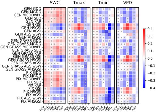
Figure 6.
Pearson correlation coefficients between model residuals and monthly meteorological (Tmin, Tmax, VPD, and SWC) anomalies for the models and for the different optimization approaches. Rows represent models, while columns correspond to months. The color scale indicates the direction and strength of the correlation (red = positive, blue = negative). The residual increases as the correlation strengthens, and vice versa. Statistically significant correlations (p < 0.05) are marked with grey dots.
During the winter period (November–December), the correlations between the residual and the selected predictors are consistently weak (but in many cases significant). This suggests that the dormant period has only a minor influence on the model error. As the season progresses into late winter and early spring (February–April), the strength of the correlations increases notably across most models and variables. This pattern suggests that environmental conditions during this pre-season period exert a stronger influence on the model–observation discrepancies in SOS estimation. In particular, the correlations become most pronounced in March and April, coinciding with the typical timing of SOS.
Distinct differences emerge among the predictors. In April, anomalies in SWC are predominantly positively correlated with the model residuals, whereas the other variables (Tmin, Tmax, and VPD) exhibit mainly negative correlations. Negative correlation means that the monthly meteorological anomaly and the residual changes are in opposite directions. For example, a warmer-than-average month means that the model predicted the SOS date earlier than the observation, or if a month was colder than average, the modeled SOS was later than the remote sensing-based SOS date.
Around April, which corresponds to the average SOS date, a general change in correlation sign can be observed. After this point, in May, several relationships change direction relative to the pre-SOS period. It is important to note that correlations for May are based only on sites and years where remote sensing-based SOS had not yet occurred earlier. While this restriction must be considered when interpreting the results, the observed sign reversal may still reflect a broader seasonal shift in the factors influencing SOS prediction errors.
Overall evaluation suggests that models with fewer parameters and single-variable dependence (e.g., GDD, MGDD, SEQ, and PAR) show stronger and more consistent correlations with the anomalies. This indicates that these simple formulations are more directly influenced by interannual variability in single meteorological drivers. However, because they lack explicit representations of additional limiting factors, such as soil moisture or photoperiod sensitivity, this leads to systematic biases under anomalous climatic conditions (e.g., unusually warm, cold, dry, or moist years). Such biases arise from the reduced ability to capture environmental variability.
Conversely, more complex models with a higher number of parameters and multiple environmental constraints (e.g., GSI, HSGSI, AGSI, AHSGSI, and AGSIwSW) generally exhibit weaker and less consistent correlations with individual anomalies. This indicates that these models can buffer or compensate for short-term anomalies through the integration of multiple drivers and longer accumulation windows.
3.5. Corrected Models and Their Evaluation
Building on the residual analysis, the identified co-variations were used to improve model performance. Linear regression models were constructed for each selected model to quantify the relationship between residuals and the meteorological and environmental anomalies (Tmin, Tmax, VPD, and SWC), with predictor variables selected based on prior correlation analysis (Figure 6). Anomalies were computed for months that could plausibly influence the timing of SOS (more precisely, the error of a given model predicting SOS), based on the condition that SOS occurred after the given month. The derived regression coefficients were then applied to adjust the raw model outputs. Note that multiple linear regression methods were also tested, including additional covariates, but the improvement was small relative to the simple linear regression.
The corrected SOS values () are obtained as:
where is the SOS value calculated by the original phenology model (e.g., GDD), is the predicted model residual as a function of monthly meteorological anomalies. Table 5 presents the constructed correction equations for the given SOS models. The coefficients in reflect the sensitivity of each model to these anomalies.
Table 5.
Linear regression-based correction equations estimating SOS model errors for selected phenological models. is the predicted model residual, and denotes the minimum and maximum temperature anomalies, while refers to the anomaly in soil water content [m3/m3]. Upper indices indicate the corresponding month for each anomaly variable.
The application of the residual correction equations effectively eliminated bias across all models. Notable improvements in overall model performance were also observed for specific cases, particularly for the GEN GRASS MGDD and GEN GRASS HSGSI models, where the RMSE decreased by approximately 4 and 3 days, respectively (see Supplementary Materials Table S7 and for additional analysis see Figures S18–S21). For the remaining models, changes in RMSE and R2 were minor, indicating that while the corrections efficiently removed bias, they had a limited influence on the spatial SOS patterns.
The following example provides a representation of the complete SOS estimation using the proposed method. The adjustable parameters—which can be generic (GEN), grassland-type dependent (GEN GRASS), or pixel-level (PIX)—are selected from Supplementary Materials Tables S8 and S9. In the case of the GEN GDD model, the parameters are and , as expressed in Equation (4):
where and is the day of SOS that is found when the inequality is fulfilled. After applying Equation (4), has to be determined based on Table 5 following Equation (5). For the GEN GDD, the correction factor depends on the SWC anomaly in April. This factor is subtracted from the GEN GDD modeled SOS, resulting in the bias-corrected model output:
4. Discussion
4.1. Remote Sensing-Based SOS Estimation
In the present study, we selected a commonly used, satellite-based measure to estimate the SOS for diverse, drought-prone, Central European grasslands. Several studies indicated that remote sensing-based SOS provides consistent results with the ground observations [25,60], or at least consistent with some measure of the SOS (see above). While datasets with higher spatial resolution are available, such as Sentinel-2-based VIs [61], the longer temporal record of MODIS offers a more robust basis for phenological modeling and has proven to be a reliable source for spatio-temporal analyses of phenological processes [8,37,62]. Nevertheless, Sentinel-2 data have shown strong potential for retrieving biophysical and physiological vegetation parameters relevant to phenology [61]. As the Sentinel-2 dataset becomes longer, new opportunities will open to quantify even sub-parcel-based phenology.
While MODIS NDVI provides a consistent, long-term record since 2000 for monitoring grassland phenology, several uncertainties must be acknowledged. The 250 m spatial resolution can cause mixed-pixel effects in heterogeneous landscapes, potentially shifting SOS estimates by several days [63]. To minimize this effect along with the known geolocation inaccuracy of the MODIS sensor [64] and the artifacts of the gridding procedure [65], we used only pixels with a high share (>90%) of the given grassland categories within the pixels but also within the side-neighboring pixels (>70%), similarly to the criterion successfully applied by Kern et al. (2022) [66]. However, despite the strict criteria used, uncertainties in SOS derivation still remain. NDVI is also influenced by soil background and atmospheric effects, which can introduce small but systematic biases even after quality filtering [67]. In addition, SOS estimates depend strongly on the detection method applied. Threshold-based metrics (e.g., G50) tend to capture the midpoint of greening, whereas curve-fitting or derivative-based approaches may identify earlier or later transition points depending on smoothing parameters and data gaps. Comparative analyses have shown that algorithm choice alone can shift SOS timing by up to several weeks in grasslands [11,36]. Therefore, while the MODIS-based SOS used here is internally consistent and suitable for regional trend analysis, it should be interpreted as one method-specific representation of greening onset rather than an absolute measure of biological activity.
Our study emphasizes the need for ancillary data (e.g., additional meteorological data other than temperature, soil texture, and soil water content) that is supposed to have similar spatial resolution to the remote sensing dataset to provide better insights. Moreover, biodiversity-related remote sensing information might also enhance the possibilities of even more sophisticated SOS modeling approaches.
4.2. Comparison with Other Studies
Grassland SOS has been modeled with several approaches in the literature. Traditionally, heat-sum formulations (GDD and MGDD) served as baselines, but even when augmented with photoperiod, they often underperform in grasslands [22,62,68]. In water-limited regions, AGSI-type models driven by vapor-pressure deficit or soil water content tend to perform better (Xin et al., 2015 [62]; RMSE ~18 days). For Mediterranean climates, the Mediterranean Grassland Phenology Model employs a soil water-potential threshold as a direct SOS trigger and reduces error to about 20–26 days compared with fixed-date baselines [69]. The Unified Model [47] variants extend temperature-based logic with hydrological cues, and the precipitation-driven UMPD explicitly accounts for short-term rainfall pulses and preseason totals, markedly improving accuracy (RMSE ≈ 9.9 days, R ≈ 0.6; [70]).
Large-scale comparisons reinforce these patterns. Post et al. (2022) [71] found that adding water availability and optimizing by Köppen climate classes yielded high R2 (0.85–0.93) in predicting grassland SOS. Dou et al. (2025) [72] reported the best-case RMSE around 5 days within a multi-model framework focusing on Central Asia. Mo et al. (2023) [22] showed that even an improved GDD ([68]) achieved only moderate accuracy in Northeast Asia (RMSE ≈ 14 days, R ≈ 0.43). White et al. (1997) [19] created an early regional model with ~6-day mean absolute error, and Tao et al. (2020) [73] demonstrated that soil moisture is more influential than temperature in Inner Mongolia in the context of SOS.
In this study, the best-performing models were MGDDwPP and AGSIwSW under GEN (RMSE = 7.6 days), AGSIwSW under GEN GRASS (RMSE = 6.3 days), and AHSGSI under PIX (RMSE = 3.3 days). Overall, we eliminated bias across all ten phenological models under three calibration types. Compared with previous studies, our results confirm that integrating water-related variables and optimizing parameter sets across multiple calibration schemes can enhance SOS prediction accuracy in grasslands.
Although the statistical indicators themselves are well defined that are used to evaluate model performance, caution is required when comparing results, since they may refer to different contexts, e.g., site-specific versus gridded approaches, spatial versus temporal averages, or metrics calculated from full time series versus subset periods. For example, in many cases model optimization and statistical evaluation are performed on the same dataset, ignoring independent validation. Harmonization of model optimization and evaluation are highly needed for better comparability of the studies.
4.3. Residual Patterns Across Models and Calibrations
Residual analysis revealed notable co-variations between model errors and key climatic variables. The simpler, temperature-driven models (GEN GDD, GEN MGDD, GEN MGDDwPP, GEN SEQ, and GEN PAR) responded primarily to SWC anomalies, showing positive relationships between residuals and SWC in April. This indicates that, for these generalized calibrations, moisture variability plays a key role in explaining the deviations between modeled and observed SOS.
Simpler, temperature-based models often fail to capture this variability, as noted by Blümel and Chmielewski (2012) [68] and Mo et al. (2023) [22], highlighting that purely thermal formulations overlook water-related constraints on vegetation activity. Similar spatially structured effects of temperature and moisture on SOS were reported by Ren et al. (2018) [74], who demonstrated that the interplay between thermal and hydrological conditions determines much of the regional variation in grassland phenology across the Northern Hemisphere. This is consistent with Tao et al. (2020) [73], who found that soil moisture exerts a stronger and more consistent influence on SOS than temperature in temperate grasslands, particularly in water-limited ecosystems. Our findings of soil moisture–linked residuals further align with Moore et al. (2015) [75], who showed that plant growth initiation in semiarid grasslands occurs only when both soil temperature and soil water content exceed threshold levels, underscoring the co-limiting nature of thermal and hydrological factors.
For the model types that are based on heat accumulation (GDD, MGDD, MGDDwPP, SEQ, and PAR) under GEN GRASS and PIX calibration, the dominance of Tmax anomalies over SWC in the residual correction equations does not necessarily imply that grass phenology is less moisture-dependent. Rather, it likely reflects that vegetation-type- and pixel-specific parameterization captures a greater share of the spatial variability in moisture conditions. Consequently, residuals become less correlated by SWC anomalies, and the remaining deviations are more closely linked to short-term thermal variability. The substantial improvement achieved through PIX-level calibration reinforces the importance of regionalized and spatially explicit parameterization, in line with large-scale assessments showing that climate-zone or biome-specific optimization markedly reduces systematic errors [71,72]. Furthermore, the increasing importance of soil-related predictors identified in our residuals supports recent evidence by Sun et al. (2025) [76], who found that including soil energetic state variables (enthalpy, moisture, and texture) enhances SOS prediction accuracy by more than 10%.
In contrast, the GSI and HSGSI models consistently used Tmin as the bias correction factor across all calibration schemes. Because Tmin is one of the internal drivers of these GSI-type formulations, the observed correlation reflects the misrepresentation of Tmin in the model structure rather than an external climatic control.
The accumulated bioclimatic index models (AGSI, AGSIwSW, and AHSGSI) contained correction terms based on Tmax anomalies, typically with small and negative coefficients, indicating that Tmax has only a minor effect on the residuals. Note that Tmax is indirectly represented in AHSGSI via Tavg, suggesting that heat accumulation can be an appropriate form of the temperature representation in phenology models. This pattern indicates that these accumulation-based formulations are less responsive to individual monthly anomalies, as the temporal integration of bioclimatic inputs improves the predictive accuracy [62].
Overall, these results confirm that soil moisture availability remains a primary constraint in water-limited grasslands, while short-term temperature fluctuations govern residual variability once the dominant moisture signal is accounted for. Integrating such relationships into model construction/calibration or bias-correction frameworks could therefore help reduce systematic model errors and improve the SOS simulations across heterogeneous grassland ecosystems. Nonetheless, the reliability of phenological simulations mainly depends on how the model structure represents real ecosystem processes. Even when environmental drivers such as temperature, SWC, and photoperiod are properly characterized, considerable deviations may occur if the mathematical formulations of the models do not capture the phenological dynamics of the vegetation [4,15,18]. This highlights the need to further develop new models or to regionalize and recalibrate existing ones, ensuring that they better capture regional vegetation-climate interactions.
4.4. Limitations and Outlook
In the context of climate change impact assessment, Piermattei (2024) [77] emphasized that precise definitions are essential to develop ecosystem models and to validate remote sensing indices. In this study, SOS was defined as the middle of intensive growth, and the models were calibrated accordingly (see also Section 4.1). Having a consistent and widely accepted definition is particularly important, since in ecosystem modeling even a few weeks’ discrepancy in the SOS can lead to substantial errors in the estimates of carbon balance, water cycling, and productivity [78].
According to the USA National Phenology Network, phenophase currently has no single, standardized definition, as the term has been used in different ways, yet it is defined as: “An observable stage or phase in the annual life cycle of a plant or animal that can be defined by a start and end point. Phenophases generally have a duration of a few days or weeks.” (https://www.usanpn.org/taxonomy/term/16, accessed on 27 August 2025) This highlights how complex the definition of SOS can be; the challenges lie not only in model development but also in the interpretation of observations, the variability among species and regions, and the choice of appropriate indicators. For instance, even in satellite-based vegetation indices, the physical environment can substantially affect how SOS is detected. In response to milder winters and reduced snow cover, it is increasingly observed that the wintertime NDVI minimum rises, resulting in a lower seasonal NDVI amplitude. This phenomenon has been reported in remote sensing studies showing that snow cover removal or reduction increases the baseline NDVI in winter, thereby decreasing the contrast between dormant and growing seasons [79]. Similarly, Gerard et al. (2020) [80] proposed that interannual changes in seasonal NDVI amplitude derived from MODIS NDVI time series can significantly influence the timing of phenological metrics based on relative thresholds. Our approach therefore identifies a point in time when the grasslands are securely active, which is a practical and consistent indicator for large-scale analyses.
The precise definition of SOS should always be tailored to the modeling needs. For example, a more detailed characterization of the SOS is needed for carbon budget studies. SOS provides information about the beginning of the growth but not about the dynamics of greening. The green-up duration (GUD), as demonstrated by Kern et al. (2020) [9], complements SOS date estimation by describing the pace and length of vegetation development, offering deeper insight into ecosystem dynamics. Although Kern et al. (2020) [9] applied this concept to deciduous forests, the same framework could be adapted to grasslands. Once GUD is quantified, the early phase of the intensive growth can be captured with a simple correction of the SOS date that is quantified in this study. Based on the preliminary analysis, the average GUD of Hungarian grasslands was 34 days for the 2000–2023 period (unpublished data). In this study, SOS was defined as the midpoint of the green-up phase; therefore, the onset of green-up can be robustly estimated by subtracting 17 days from the SOS date, independent of interannual variability.
Another major limitation is the relatively coarse resolution of the applied meteorological dataset that is clearly unable to capture small-scale variability caused by, e.g., topography and soil conditions. In this sense, construction of climate datasets that can better characterize microclimate might enhance the applicability of the SOS models. In addition to this, the combined use of datasets with different spatial resolutions (MODIS at 250 m, SWC at 0.25°, and meteorological variables at 0.1°) can also introduce scale-related uncertainties. Fine-scale phenological dynamics captured by MODIS may be spatially smoothed when linked to coarser SWC or meteorology. This effect can weaken SOS-environment relationships. Also, currently available SWC datasets have limited applicability (e.g., remote sensing datasets only characterize the topsoil that might not be a good indicator of the overall water availability of the grasslands, including new global products such as S1-DPA; [81]). One possible option is the exploitation of reanalysis-based SWC, although those datasets are typically modeled with limited information content. New, fine resolution SWC datasets are highly needed for improved model construction and parameterization. For example, the so-called Operational drought and water scarcity management system (https://aszalymonitoring.vizugy.hu/, accessed on 14 December 2025) in Hungary provides in situ SWC data for 127 locations in the country that offers options to harmonize remote sensing data and interpolated in situ observations.
The PIX-level calibration provides a solid database where model parameterization is available for the whole country. The spatial information content of the parameters can provide an additional basis for improved model construction.
5. Conclusions
In this study, we estimated the SOS date for Hungarian grasslands using satellite-derived data. Following the establishment of the SOS reference dataset, we calibrated ten process-based phenology models using three different strategies based on an advanced differential evolution genetic algorithm. According to the knowledge of the authors, this was the first study to apply evolutionary algorithms for modeling SOS in grassland ecosystems.
Although temperature is included as a key driver in the applied phenology models, neither heat sum-based nor bioclimatic index approaches were able to adequately capture its influence on SOS, suggesting that temperature effects should be incorporated differently in future models. Residual analysis allowed us to identify systematic relationships between model errors and climate anomalies, which were subsequently used to implement bias corrections that effectively reduced average errors to zero. Clearly, more advanced models with in-depth process understanding are needed for better, spatially applicable models.
Overall, our results demonstrate that SOS date in drought-prone, semi-arid Central European grasslands can be relatively well modeled when both fine-scale calibration and spatially explicit environmental information are considered. The modeling framework presented here offers a robust and scalable approach for predicting vegetation SOS, supporting future applications in phenology modeling, carbon cycle studies, and climate adaptation research. Finally, we provide a ready-to-use algorithm for the SOS modeling that can be easily incorporated into existing biogeochemical and biophysical models.
Supplementary Materials
The following supporting information can be downloaded at: https://www.mdpi.com/article/10.3390/atmos17010049/s1, [19,23,50,58,62,82,83,84,85], Figure S1: Kernel density estimates (KDEs) of SOS date values (expressed as DOY) for the different grassland types. Salt steppes and meadows (grasslands affected by salinization included) typically exhibit earlier green-up compared to the other types; Table S1: Statistical indicators of the remote sensing-based SOS values for grasslands, where P1, P5, P95, and P99 denote the first, fifth, 95th, and 99th percentiles, respectively; Table S2: Basic statistics for GEN calibrated models, where P1, P5, P95, and P99 denote the first, fifth, 95th, and 99th percentiles, respectively; Table S3: Basic statistics for GEN GRASS calibrated models, where P1, P5, P95, and P99 denote the first, fifth, 95th, and 99th percentiles, respectively; Table S4: Basic statistics for PIX calibrated models, where P1, P5, P95, and P99 denote the first, fifth, 95th, and 99th percentiles, respectively; Table S5: Pairwise comparisons of grassland types using Dunn’s test with Bonferroni correction; Figure S2: Comparison of the modeled and observed temporal mean SOS values from the GEN calibrations, where each point represents a 5-year average for a single pixel. Pearson r2, bias, and RMSE values are shown; Figure S3: Comparison of the modeled and observed temporal mean SOS values from the GEN GRASS calibrations, where each point represents a 5-year average for a single pixel. Pearson r2, bias, and RMSE values are shown; Figure S4: Comparison of the modeled and observed temporal mean SOS values from the PIX calibrations, where each point represents a 5-year average for a single pixel. Pearson r2, bias, and RMSE values are shown; Figure S5. Spatial comparison of the observed and modeled SOS based on the GEN calibration. Each point represents the annual average of approximately 12,000 pixels. Gray points represent training data, and blue points indicate validation years. The dashed line denotes the 1:1 relationship, while the solid line is the result of the linear regression. Statistical metrics (Pearson r2, bias, and RMSE) are reported for the full dataset (including training and validation years), with test-year values highlighted in blue; Figure S6: Spatial scatterplots of grassland-type-specific general calibrations. Each point represents the annual average of ~12,000 pixels. Gray points represent training data, and blue points indicate validation years. The dashed line denotes the 1:1 relationship, while the solid line is the result of the linear regression. Statistical metrics (Pearson r2, bias, and RMSE) are reported for the full dataset (including training and validation years), with test-year values highlighted in blue. Figure S7. Spatial scatterplots of pixel-level calibrations. Each point corresponds to the annual average of approximately 12,000 pixels. Gray points represent training data, and blue points indicate validation years. The dashed line denotes the 1:1 relationship, while the solid line is the result of the linear regression. Statistical metrics (Pearson r2, bias, and RMSE) are reported for the full dataset (including training and validation years), with test-year values highlighted in blue; Table S6. Pearson r values for each phenology model under three calibration schemes (GEN, GEN GRASS, and PIX) were computed using data from the validation years. The statistics represent pixel-level performance, quantifying the spatial correspondence of SOS patterns across models computed from independent validation years; Table S7: Statistics for each phenology model and the corrected models under three calibration schemes (GEN, GEN GRASS, and PIX) computed using data from all years. Note that the statistical values presented here differ from Tables 2 and S6 because those are calculated only for the validation years. The statistics represent pixel-level performance, quantifying the spatial correspondence of SOS patterns across models based on independent validation data; Figures S8–S17: Violin plots (for GDD, MGDD, MGDDwPP, SEQQ, PAR, GSI, HSGSI, AGSIwSW, AGSI, and AHSGSI models) illustrating the distribution of PIX-calibrated parameters for the AHSGSI model. The black vertical line represents the GEN calibration value, while the blue, pink, green, and yellow vertical lines indicate the GEN GRASS calibrated parameters for Open sand steppes, Closed sand steppes, Salt steppes and meadows (grasslands affected by salinization included), and Closed grasslands in hills and mountains or on cohesive soil, respectively; Table S8: Parameter intervals (minimum-maximum) for the heat accumulation-based models. The numbers displayed beneath each parameter name represent the parameter intervals: the left-hand value indicates the minimum (lower bound), and the right-hand value indicates the maximum (upper bound). The ranges were determined from expert knowledge, published literature, and empirical experience. Within each model type (GDD, MGDD, MGDDwPP, SEQ, and PAR), the GEN, GEN GRASS, and PIX rows correspond to the parameter sets used for different calibration categories; Table S9: Parameter intervals (minimum-maximum) for the GSI-type models. The numbers displayed beneath each parameter name represent the parameter intervals: the left-hand value indicates the minimum (lower bound), and the right-hand value indicates the maximum (upper bound). The ranges were determined from expert knowledge, published literature, and empirical experience. Within each model type (GSI, AGSI, AGSIwSW, HSGSI, and AHGSI), the GEN, GEN GRASS, and PIX rows correspond to the parameter sets used for different calibration categories. Figure S18. Performance of the evaluated models for Open sand steppes, shown in terms of bias and RMSE before (Original) and after bias correction (Corrected). Each point represents a model, while dashed vertical lines connect original and corrected values for the same model to enhance visual clarity. Figure S19. Performance of the evaluated models for Closed sand steppes, shown in terms of bias and RMSE before (Original) and after bias correction (Corrected). Each point represents a model, while dashed vertical lines connect original and corrected values for the same model to enhance visual clarity. Figure S20. Performance of the evaluated models for Salt steppes and meadows (grasslands affected by salinisation included), shown in terms of bias and RMSE before (Original) and after bias correction (Corrected). Each point represents a model, while dashed vertical lines connect original and corrected values for the same model to enhance visual clarity. Figure S21. Performance of the evaluated models for Closed grasslands in hills and mountains or on cohesive soil, shown in terms of bias and RMSE before (Original) and after bias correction (Corrected). Each point represents a model, while dashed vertical lines connect original and corrected values for the same model to enhance visual clarity.
Author Contributions
Conceptualization, Z.B. and R.Á.D.; methodology, Z.B., R.Á.D. and R.H.; software, R.Á.D. and R.H.; validation, R.Á.D., Z.B. and A.K.; formal analysis, R.Á.D.; investigation, R.Á.D., Z.B. and R.H.; resources, Z.B.; data curation, R.Á.D. and A.K.; writing—original draft preparation, R.Á.D. and Z.B.; writing—review and editing, R.Á.D., Z.B., A.K. and R.H.; visualization, R.Á.D.; supervision, Z.B.; project administration, Z.B.; funding acquisition, Z.B. All authors have read and agreed to the published version of the manuscript.
Funding
The research was funded by the Ministry of Culture and Innovation, National Research Development and Innovation Fund, under the University Research Fellowship Program. The research has been supported by the Hungarian National Scientific Research Fund (NKFIH FK-146600) and the TKP2021-NVA-29 project of the Hungarian National Research, Development and Innovation Fund, with the support provided by the Ministry of Culture and Innovation of Hungary. This work has been implemented by the National Multidisciplinary Laboratory for Climate Change (RRF-2.3.1-21-2022-00014) project within the framework of Hungary’s National Recovery and Resilience Plan supported by the Recovery and Resilience Facility of the European Union. This work was also supported by the FK 131813 project, implemented with support provided by the National Research, Development and Innovation Fund of Hungary, financed under the FK_19 funding scheme. RH and ZB were supported by the “Advanced methods of greenhouse gases emission reduction and sequestration in agriculture and forest landscape for climate change mitigation” (CZ.02.01.01/00/22_008/0004635) project. Support was also provided by the TKP2021-NKTA-06 project that has been implemented with the support provided by the Ministry of Innovation and Technology of Hungary from the National Research, Development and Innovation Fund, financed under the [TKP2021-NKTA] funding scheme. Also supported by the French-Hungarian bilateral partnership through the BALATON (N° 44703TF)/TéT (2019-2.1.11-TÉT-2019-00031) program.
Institutional Review Board Statement
Not applicable.
Informed Consent Statement
Not applicable.
Data Availability Statement
The presented dataset is available from the authors upon request.
Acknowledgments
We acknowledge the use of the MODIS MOD09Q1 (Collection 6.1) dataset provided by NASA. This study utilized the FORESEE-HUN v1.2 climate database developed at Eötvös Loránd University. We also acknowledge the European Space Agency’s Climate Change Initiative (ESA CCI) for providing the Soil Moisture COMBINED v09.1 dataset. The Hungarian Ecosystem Map (NÖSZTÉP) was provided by the NÖSZTÉP Project, integrating national databases and Sentinel satellite data (2015–2017). During the preparation of this manuscript/study, the author(s) used ChatGPT (GPT-5) for the purposes of improving the academic English language of the text and assisting in the generation and refinement of figures through scripting support. The authors have reviewed and edited the output and take full responsibility for the content of this publication.
Conflicts of Interest
The authors declare no conflicts of interest.
Abbreviations
The following abbreviations are used in this manuscript:
| AGSI | Accumulated Heat Sum Growing Season Index |
| AGSIwSW | Accumulated Heat Sum Growing Season Index Model with Soil Water Content |
| AHSGSI | Accumulated Heat Sum Growing Season Index |
| ENS | Model Ensembles |
| GDD | Growing Degree Days |
| GSI | Heat Sum Growing Season Index |
| HSGSI | Heat Sum Growing Season Index |
| MGDD | Modified Growing Degree Days |
| MGDDwPP | Modified Growing Degree Days with Photoperiod |
| PAR | Parallel |
| PP | Photoperiod |
| SEQ | Sequential |
| SWC | Soil water content |
| Tavg | Average temperature |
| Tmax | Maximum temperature |
| Tmin | Minimum temperature |
| VPD | Vapor pressure deficit |
References
- Caparros-Santiago, J.A.; Rodriguez-Galiano, V.; Dash, J. Land Surface Phenology as Indicator of Global Terrestrial Ecosystem Dynamics: A Systematic Review. ISPRS J. Photogramm. Remote Sens. 2021, 171, 330–347. [Google Scholar] [CrossRef]
- Richardson, A.D.; Keenan, T.F.; Migliavacca, M.; Ryu, Y.; Sonnentag, O.; Toomey, M. Climate Change, Phenology, and Phenological Control of Vegetation Feedbacks to the Climate System. Agric. For. Meteorol. 2013, 169, 156–173. [Google Scholar] [CrossRef]
- Stuble, K.L.; Bennion, L.D.; Kuebbing, S.E. Plant Phenological Responses to Experimental Warming—A Synthesis. Glob. Change Biol. 2021, 27, 4110–4124. [Google Scholar] [CrossRef] [PubMed]
- Fu, Y.; Zhang, H.; Dong, W.; Yuan, W. Comparison of Phenology Models for Predicting the Onset of Growing Season over the Northern Hemisphere. PLoS ONE 2014, 9, e109544. [Google Scholar] [CrossRef]
- Jánosi, I.M.; Silhavy, D.; Tamás, J.; Csontos, P. Bulbous Perennials Precisely Detect the Length of Winter and Adjust Flowering Dates. New Phytol. 2020, 228, 1343–1351. [Google Scholar] [CrossRef]
- Templ, B.; Koch, E.; Bolmgren, K.; Ungersböck, M.; Paul, A.; Scheifinger, H.; Rutishauser, T.; Busto, M.; Chmielewski, F.M.; Hájková, L.; et al. Pan European Phenological Database (PEP725): A Single Point of Access for European Data. Int. J. Biometeorol. 2018, 62, 1109–1113. [Google Scholar] [CrossRef]
- Tóth, V.R. Monitoring Spatial Variability and Temporal Dynamics of Phragmites Using Unmanned Aerial Vehicles. Front. Plant. Sci. 2018, 9, 728. [Google Scholar] [CrossRef]
- Bellini, E.; Moriondo, M.; Dibari, C.; Leolini, L.; Staglianò, N.; Stendardi, L.; Filippa, G.; Galvagno, M.; Argenti, G. Impacts of Climate Change on European Grassland Phenology: A 20-Year Analysis of MODIS Satellite Data. Remote Sens. 2023, 15, 218. [Google Scholar] [CrossRef]
- Kern, A.; Marjanović, H.; Barcza, Z. Spring Vegetation Green-up Dynamics in Central Europe Based on 20-Year Long MODIS NDVI Data. Agric. For. Meteorol. 2020, 287, 107969. [Google Scholar] [CrossRef]
- Ma, X.; Zhu, X.; Xie, Q.; Jin, J.; Zhou, Y.; Luo, Y.; Liu, Y.; Tian, J.; Zhao, Y. Monitoring Nature’s Calendar from Space: Emerging Topics in Land Surface Phenology and Associated Opportunities for Science Applications. Glob. Change Biol. 2022, 28, 7186–7204. [Google Scholar] [CrossRef]
- White, M.A.; de Beurs, K.M.; Didan, K.; Inouye, D.W.; Richardson, A.D.; Jensen, O.P.; O’Keefe, J.; Zhang, G.; Nemani, R.R.; van Leeuwen, W.J.D.; et al. Intercomparison, Interpretation, and Assessment of Spring Phenology in North America Estimated from Remote Sensing for 1982–2006. Glob. Change Biol. 2009, 15, 2335–2359. [Google Scholar] [CrossRef]
- Xu, J.; Tang, Y.; Xu, J.; Chen, J.; Bai, K.; Shu, S.; Yu, B.; Wu, J.; Huang, Y. Evaluation of Vegetation Indexes and Green-Up Date Extraction Methods on the Tibetan Plateau. Remote Sens. 2022, 14, 3160. [Google Scholar] [CrossRef]
- Aono, Y.; Saito, S. Clarifying Springtime Temperature Reconstructions of the Medieval Period by Gap-Filling the Cherry Blossom Phenological Data Series at Kyoto, Japan. Int. J. Biometeorol. 2010, 54, 211–219. [Google Scholar] [CrossRef] [PubMed]
- Chuine, I.; Yiou, P.; Viovy, N.; Seguin, B.; Daux, V.; Le Roy Ladurie, E. Grape Ripening as a Past Climate Indicator. Nature 2004, 432, 289–290. [Google Scholar] [CrossRef] [PubMed]
- Piao, S.; Liu, Q.; Chen, A.; Janssens, I.A.; Fu, Y.; Dai, J.; Liu, L.; Lian, X.; Shen, M.; Zhu, X. Plant Phenology and Global Climate Change: Current Progresses and Challenges. Glob. Change Biol. 2019, 25, 1922–1940. [Google Scholar] [CrossRef]
- Peaucelle, M.; Janssens, I.A.; Stocker, B.D.; Descals Ferrando, A.; Fu, Y.H.; Molowny-Horas, R.; Ciais, P.; Peñuelas, J. Spatial Variance of Spring Phenology in Temperate Deciduous Forests Is Constrained by Background Climatic Conditions. Nat. Commun. 2019, 10, 5388. [Google Scholar] [CrossRef]
- Tang, J.; Körner, C.; Muraoka, H.; Piao, S.; Shen, M.; Thackeray, S.J.; Yang, X. Emerging Opportunities and Challenges in Phenology: A Review. Ecosphere 2016, 7, e01436. [Google Scholar] [CrossRef]
- Wu, M.; Vico, G.; Manzoni, S.; Cai, Z.; Bassiouni, M.; Tian, F.; Zhang, J.; Ye, K.; Messori, G. Early Growing Season Anomalies in Vegetation Activity Determine the Large-Scale Climate-Vegetation Coupling in Europe. J. Geophys. Res. Biogeosci. 2021, 126, e2020JG006167. [Google Scholar] [CrossRef]
- White, M.A.; Thornton, P.E.; Running, S.W. A Continental Phenology Model for Monitoring Vegetation Responses to Interannual Climatic Variability. Glob. Biogeochem. Cycles 1997, 11, 217–234. [Google Scholar] [CrossRef]
- Ahlström, A.; Raupach, M.R.; Schurgers, G.; Smith, B.; Arneth, A.; Jung, M.; Reichstein, M.; Canadell, J.G.; Friedlingstein, P.; Jain, A.K.; et al. The Dominant Role of Semi-Arid Ecosystems in the Trend and Variability of the Land CO2 Sink. Science 2015, 348, 895–899. [Google Scholar] [CrossRef]
- Wu, W.; Sun, Y.; Xiao, K.; Xin, Q. Development of a Global Annual Land Surface Phenology Dataset for 1982–2018 from the AVHRR Data by Implementing Multiple Phenology Retrieving Methods. Int. J. Appl. Earth Obs. Geoinf. 2021, 103, 102487. [Google Scholar] [CrossRef]
- Mo, Y.; Zhang, J.; Jiang, H.; Fu, Y.H. A Comparative Study of 17 Phenological Models to Predict the Start of the Growing Season. Front. For. Glob. Change 2023, 5, 1032066. [Google Scholar] [CrossRef]
- Hidy, D.; Barcza, Z.; Haszpra, L.; Churkina, G.; Pintér, K.; Nagy, Z. Development of the Biome-BGC Model for Simulation of Managed Herbaceous Ecosystems. Ecol. Model. 2012, 226, 99–119. [Google Scholar] [CrossRef]
- Eklundh, L.; Jönsson, P. Timesat for Processing Time-Series Data from Satellite Sensors for Land Surface Monitoring. Remote Sens. Digit. Image Process. 2016, 20, 177–194. [Google Scholar] [CrossRef]
- Balzarolo, M.; Vicca, S.; Nguy-Robertson, A.L.; Bonal, D.; Elbers, J.A.; Fu, Y.H.; Grünwald, T.; Horemans, J.A.; Papale, D.; Peñuelas, J.; et al. Matching the Phenology of Net Ecosystem Exchange and Vegetation Indices Estimated with MODIS and FLUXNET In-Situ Observations. Remote Sens. Environ. 2016, 174, 290–300. [Google Scholar] [CrossRef]
- Kern, A.; Marjanović, H.; Barcza, Z. Evaluation of the Quality of NDVI3g Dataset against Collection 6 MODIS NDVI in Central Europe between 2000 and 2013. Remote Sens. 2016, 8, 955. [Google Scholar] [CrossRef]
- Belényesi, M.; Pacskó, V.; Lehoczki, R.; Pataki, R.; Tanács, E.; Kristóf, D.; Szekeres, Á.; Zsembery, Z.; Mikus, G. National Grassland Mapping in Hungary: Status Report. Tájökológiai Lapok J. Landsc. Ecol. 2025, 23, 3–45. [Google Scholar] [CrossRef]
- Kroël-Dulay, G.; Ransijn, J.; Schmidt, I.K.; Beier, C.; De Angelis, P.; De Dato, G.; Dukes, J.S.; Emmett, B.; Estiarte, M.; Garadnai, J.; et al. Increased Sensitivity to Climate Change in Disturbed Ecosystems. Nat. Commun. 2015, 6, 6682. [Google Scholar] [CrossRef]
- Orbán, I.; Ónodi, G.; Kröel-Dulay, G. The Role of Drought, Disturbance, and Seed Dispersal in Dominance Shifts in a Temperate Grassland. J. Veg. Sci. 2023, 34, e13199. [Google Scholar] [CrossRef]
- Barcza, Z.; Haszpra, L.; Kondo, H.; Saigusa, N.; Yamamoto, S.; Bartholy, J. Carbon Exchange of Grass in Hungary. Tellus B Chem. Phys. Meteorol. 2003, 55, 187–196. [Google Scholar] [CrossRef]
- Nagy, Z.; Pintér, K.; Czóbel, S.; Balogh, J.; Horváth, L.; Fóti, S.; Barcza, Z.; Weidinger, T.; Csintalan, Z.; Dinh, N.Q.; et al. The Carbon Budget of Semi-Arid Grassland in a Wet and a Dry Year in Hungary. Agric. Ecosyst. Environ. 2007, 121, 21–29. [Google Scholar] [CrossRef]
- Nagy, Z.; Barcza, Z.; Horváth, L.; Balogh, J.; Hagyó, A.; Káposztás, N.; Béla, G.; Machon, A.; Pintér, K. Measurements and Estimations of Biosphere-Atmosphere Exchange of Greenhouse Gases–Grasslands. In Atmospheric Greenhouse Gases: The Hungarian Perspective; Haszpra, L., Ed.; Springer: Berlin/Heidelberg, Germany, 2010; pp. 91–120. ISBN 978-90-481-9959-2. [Google Scholar]
- Tanács, E.; Belényesi, M.; Lehoczki, R.; Pataki, R.; Petrik, O.; Standovár, T.; Pásztor, L.; Laborczi, A.; Szatmári, G.; Molnár, Z.; et al. Országos, Nagyfelbontású Ökoszisztéma- Alaptérkép: Módszertan, Validáció És Felhasználási Lehetőségek. Természetvédelmi Közlemények 2019, 25, 34–58. [Google Scholar] [CrossRef]
- Vermote, E.F. MODIS/Terra Surface Reflectance 8-Day L3 Global 250m SIN Grid V061; NASA Land Processes Distributed Active Archive Center: Sioux Falls, South Dakota, 2021. [Google Scholar]
- Wood, D.J.A.; Powell, S.; Stoy, P.C.; Thurman, L.L.; Beever, E.A. Is the Grass Always Greener? Land Surface Phenology Reveals Differences in Peak and Season-Long Vegetation Productivity Responses to Climate and Management. Ecol. Evol. 2021, 11, 11168–11199. [Google Scholar] [CrossRef] [PubMed]
- Zhang, X.; Friedl, M.A.; Schaaf, C.B.; Strahler, A.H.; Hodges, J.C.F.; Gao, F.; Reed, B.C.; Huete, A. Monitoring Vegetation Phenology Using MODIS. Remote Sens. Environ. 2003, 84, 471–475. [Google Scholar] [CrossRef]
- Wang, B.; Tian, Z.; Zhang, W.; Chen, G.; Guo, Y.; Wang, M. Retrieval of Green-up Onset Date from MODIS Derived NDVI in Grasslands of Inner Mongolia. IEEE Access 2019, 7, 77885–77893. [Google Scholar] [CrossRef]
- Shen, M.; Zhang, G.; Cong, N.; Wang, S.; Kong, W.; Piao, S. Increasing Altitudinal Gradient of Spring Vegetation Phenology during the Last Decade on the Qinghai-Tibetan Plateau. Agric. For. Meteorol. 2014, 189–190, 71–80. [Google Scholar] [CrossRef]
- Yu, H.; Luedeling, E.; Xu, J. Winter and Spring Warming Result in Delayed Spring Phenology on the Tibetan Plateau. Proc. Natl. Acad. Sci. USA 2010, 107, 22151–22156. [Google Scholar] [CrossRef]
- Kern, A.; Dobor, L.; Hollós, R.; Marjanović, H.; Torma, C.Z.; Kis, A.; Fodor, N.; Barcza, Z. Seamlessly Combined Historical and Projected Daily Meteorological Datasets for Impact Studies in Central Europe: The FORESEE v4.0 and the FORESEE-HUN v1.0. Clim. Serv. 2024, 33, 100443. [Google Scholar] [CrossRef]
- Gruber, A.; Scanlon, T.; Van Der Schalie, R.; Wagner, W.; Dorigo, W. Evolution of the ESA CCI Soil Moisture Climate Data Records and Their Underlying Merging Methodology. Earth Syst. Sci. Data 2019, 11, 717–739. [Google Scholar] [CrossRef]
- Dorigo, W.; Wagner, W.; Albergel, C.; Albrecht, F.; Balsamo, G.; Brocca, L.; Chung, D.; Ertl, M.; Forkel, M.; Gruber, A.; et al. ESA CCI Soil Moisture for Improved Earth System Understanding: State-of-the Art and Future Directions. Remote Sens. Environ. 2017, 203, 185–215. [Google Scholar] [CrossRef]
- Preimesberger, W.; Stradiotti, P.; Dorigo, W. ESA CCI Soil Moisture GAPFILLED: An Independent Global Gap-Free Satellite Climate Data Record with Uncertainty Estimates. Earth Syst. Sci. Data 2025, 17, 4305–4329. [Google Scholar] [CrossRef]
- Pataki, A.; Bertalan, L.; Pásztor, L.; Nagy, L.A.; Abriha, D.; Liang, S.; Singh, S.K.; Szabó, S. Soil Moisture Satellite Data Under Scrutiny: Assessing Accuracy Through Environmental Proxies and Extended Triple Collocation Analysis. Earth Syst. Environ. 2025, 9, 801–824. [Google Scholar] [CrossRef]
- Asse, D.; Randin, C.F.; Bonhomme, M.; Delestrade, A.; Chuine, I. Process-Based Models Outcompete Correlative Models in Projecting Spring Phenology of Trees in a Future Warmer Climate. Agric. For. Meteorol. 2020, 285–286, 107931. [Google Scholar] [CrossRef]
- Basler, D. Evaluating Phenological Models for the Prediction of Leaf-out Dates in Six Temperate Tree Species across Central Europe. Agric. For. Meteorol. 2016, 217, 10–21. [Google Scholar] [CrossRef]
- Chuine, I. A Unified Model for Budburst of Trees. J. Theor. Biol. 2000, 207, 337–347. [Google Scholar] [CrossRef]
- Cleland, E.E.; Chuine, I.; Menzel, A.; Mooney, H.A.; Schwartz, M.D. Shifting Plant Phenology in Response to Global Change. Trends Ecol. Evol. 2007, 22, 357–365. [Google Scholar] [CrossRef]
- Hufkens, K.; Basler, D.; Milliman, T.; Melaas, E.K.; Richardson, A.D. An Integrated Phenology Modelling Framework in r. Methods Ecol. Evol. 2018, 9, 1276–1285. [Google Scholar] [CrossRef]
- Melaas, E.K.; Richardson, A.D.; Friedl, M.A.; Dragoni, D.; Gough, C.M.; Herbst, M.; Montagnani, L.; Moors, E. Using FLUXNET Data to Improve Models of Springtime Vegetation Activity Onset in Forest Ecosystems. Agric. For. Meteorol. 2013, 171–172, 46–56. [Google Scholar] [CrossRef]
- Zhang, L.; Lei, H.; Shen, H.; Cong, Z.; Yang, D.; Liu, T. Evaluating the Representation of Vegetation Phenology in the Community Land Model 4.5 in a Temperate Grassland. J. Geophys. Res. Biogeosci. 2019, 124, 187–210. [Google Scholar] [CrossRef]
- Menzel, A.; Sparks, T.H.; Estrella, N.; Koch, E.; Aaasa, A.; Ahas, R.; Alm-Kübler, K.; Bissolli, P.; Braslavská, O.; Briede, A.; et al. European Phenological Response to Climate Change Matches the Warming Pattern. Glob. Change Biol. 2006, 12, 1969–1976. [Google Scholar] [CrossRef]
- Holland, J.H. Adaptation in Natural and Artificial Systems: An Introductory Analysis with Applications to Biology, Control, and Artificial Intelligence; The MIT Press: Cambridge, MA, USA, 1992; ISBN 9780262581110. [Google Scholar]
- Zhou, M.C.; Cui, M.; Xu, D.; Zhu, S.; Zhao, Z.; Abusorrah, A. Evolutionary Optimization Methods for High-Dimensional Expensive Problems: A Survey. IEEE/CAA J. Autom. Sin. 2024, 11, 1092–1105. [Google Scholar] [CrossRef]
- Abdel-Basset, M.; Abdel-Fatah, L.; Sangaiah, A.K. Metaheuristic Algorithms: A Comprehensive Review; Elsevier Inc.: Amsterdam, The Netherlands, 2018; ISBN 9780128133149. [Google Scholar]
- Storn, R.; Price, K. Differential Evolution—A Simple and Efficient Heuristic for Global Optimization over Continuous Spaces. J. Glob. Optim. 1997, 11, 341–359. [Google Scholar] [CrossRef]
- Virtanen, P.; Gommers, R.; Oliphant, T.E.; Haberland, M.; Reddy, T.; Cournapeau, D.; Burovski, E.; Peterson, P.; Weckesser, W.; Bright, J.; et al. SciPy 1.0: Fundamental Algorithms for Scientific Computing in Python. Nat. Methods 2020, 17, 261–272, Erratum in Nat. Methods 2020. https://doi.org/10.1038/s41592-020-0772-5. [Google Scholar] [CrossRef] [PubMed]
- Sándor, R.; Barcza, Z.; Hidy, D.; Lellei-Kovács, E.; Ma, S.; Bellocchi, G. Modelling of Grassland Fluxes in Europe: Evaluation of Two Biogeochemical Models. Agric. Ecosyst. Environ. 2016, 215, 1–19. [Google Scholar] [CrossRef]
- Akaike, H. A New Look at the Statistical Model Identification. IEEE Trans. Automat. Contr. 1974, 19, 716–723. [Google Scholar] [CrossRef]
- Zhang, X.; Friedl, M.A.; Schaaf, C.B. Global Vegetation Phenology from Moderate Resolution Imaging Spectroradiometer (MODIS): Evaluation of Global Patterns and Comparison with in Situ Measurements. J. Geophys. Res. Biogeosci. 2006, 111, 716–723. [Google Scholar] [CrossRef]
- Frampton, W.J.; Dash, J.; Watmough, G.; Milton, E.J. Evaluating the Capabilities of Sentinel-2 for Quantitative Estimation of Biophysical Variables in Vegetation. ISPRS J. Photogramm. Remote Sens. 2013, 82, 83–92. [Google Scholar] [CrossRef]
- Xin, Q.; Broich, M.; Zhu, P.; Gong, P. Modeling Grassland Spring Onset across the Western United States Using Climate Variables and MODIS-Derived Phenology Metrics. Remote Sens. Environ. 2015, 161, 63–77. [Google Scholar] [CrossRef]
- Atkinson, P.M.; Jeganathan, C.; Dash, J.; Atzberger, C. Inter-Comparison of Four Models for Smoothing Satellite Sensor Time-Series Data to Estimate Vegetation Phenology. Remote Sens. Environ. 2012, 123, 400–417. [Google Scholar] [CrossRef]
- Wolfe, R.E.; Nishihama, M.; Fleig, A.J.; Kuyper, J.A.; Roy, D.P.; Storey, J.C.; Patt, F.S. Achieving Sub-Pixel Geolocation Accuracy in Support of MODIS Land Science. Remote Sens. Environ. 2002, 83, 31–49. [Google Scholar] [CrossRef]
- Tan, B.; Woodcock, C.E.; Hu, J.; Zhang, P.; Ozdogan, M.; Huang, D.; Yang, W.; Knyazikhin, Y.; Myneni, R.B. The Impact of Gridding Artifacts on the Local Spatial Properties of MODIS Data: Implications for Validation, Compositing, and Band-to-Band Registration across Resolutions. Remote Sens. Environ. 2006, 105, 98–114. [Google Scholar] [CrossRef]
- Kern, A.; Barcza, Z.; Hollós, R.; Birinyi, E.; Marjanović, H. Critical Climate Periods Explain a Large Fraction of the Observed Variability in Vegetation State. Remote Sens. 2022, 14, 5621. [Google Scholar] [CrossRef]
- Huete, A.R.; Didan, K.; Miura, T.; Rodriguez, E.P.; Gao, X.; Ferreira, L.G. Overview of the Radiometric and Biophysical Performance of the MODIS Vegetation Indices. Remote Sens. Environ. 2002, 83, 195–213. [Google Scholar] [CrossRef]
- Blümel, K.; Chmielewski, F.M. Shortcomings of Classical Phenological Forcing Models and a Way to Overcome Them. Agric. For. Meteorol. 2012, 164, 10–19. [Google Scholar] [CrossRef]
- Bart, R.R.; Tague, C.L.; Dennison, P.E. Modeling Annual Grassland Phenology along the Central Coast of California. Ecosphere 2017, 8, e01875. [Google Scholar] [CrossRef]
- Fan, D.; Zhao, X.; Zhu, W.; Sun, W.; Qiu, Y. An Improved Phenology Model for Monitoring Green-up Date Variation in Leymus Chinensis Steppe in Inner Mongolia during 1962–2017. Agric. For. Meteorol. 2020, 291, 108091. [Google Scholar] [CrossRef]
- Post, A.K.; Hufkens, K.; Richardson, A.D. Predicting Spring Green-up across Diverse North American Grasslands. Agric. For. Meteorol. 2022, 327, 109204. [Google Scholar] [CrossRef]
- Dou, X.; Wu, L.; Zhao, C.; Li, J.; Yan, Y.; Zhu, J.; Wang, D. Comparison of Spring Phenology Simulation in Central Asian Grasslands. Ecol. Model. 2025, 501, 111011. [Google Scholar] [CrossRef]
- Tao, Z.; Huang, W.; Wang, H. Soil Moisture Outweighs Temperature for Triggering the Green-up Date in Temperate Grasslands. Theor. Appl. Climatol. 2020, 140, 1093–1105. [Google Scholar] [CrossRef]
- Ren, S.; Chen, X.; Lang, W.; Schwartz, M.D. Climatic Controls of the Spatial Patterns of Vegetation Phenology in Midlatitude Grasslands of the Northern Hemisphere. J. Geophys. Res. Biogeosci. 2018, 123, 2323–2336. [Google Scholar] [CrossRef]
- Moore, L.M.; Lauenroth, W.K.; Bell, D.M.; Schlaepfer, D.R. Soil Water and Temperature Explain Canopy Phenology and Onset of Spring in a Semiarid Steppe. Great Plains Res. 2015, 25, 121–138. [Google Scholar] [CrossRef]
- Sun, X.; Lu, N.; Shen, M.; Qin, J. Improved Modeling of Vegetation Phenology Using Soil Enthalpy. Glob. Change Biol. 2025, 31, e70116. [Google Scholar] [CrossRef] [PubMed]
- Piermattei, A. A New Perspective on Tree Growing Season Determination. J. Biogeogr. 2024, 51, 2334–2337. [Google Scholar] [CrossRef]
- Keenan, T.F.; Gray, J.; Friedl, M.A.; Toomey, M.; Bohrer, G.; Hollinger, D.Y.; Munger, J.W.; O’Keefe, J.; Schmid, H.P.; Wing, I.S.; et al. Net Carbon Uptake Has Increased through Warming-Induced Changes in Temperate Forest Phenology. Nat. Clim. Change 2014, 4, 598–604. [Google Scholar] [CrossRef]
- Wu, Y.; Xiao, P.; Zhang, X.; Liu, H.; Dong, Y.; Feng, L. Effects of Snow Cover on Spring Vegetation Phenology Vary with Temperature Gradient Across the Pan-Arctic. J. Geophys. Res. Biogeosci. 2023, 128, e2022JG007183. [Google Scholar] [CrossRef]
- Gerard, F.F.; George, C.T.; Hayman, G.; Chavana-Bryant, C.; Weedon, G.P. Leaf Phenology Amplitude Derived from MODIS NDVI and EVI: Maps of Leaf Phenology Synchrony for Meso- and South America. Geosci. Data J. 2020, 7, 13–26. [Google Scholar] [CrossRef]
- Fan, D.; Zhao, T.; Jiang, X.; García-García, A.; Schmidt, T.; Samaniego, L.; Attinger, S.; Wu, H.; Jiang, Y.; Shi, J.; et al. A Sentinel-1 SAR-Based Global 1-Km Resolution Soil Moisture Data Product: Algorithm and Preliminary Assessment. Remote Sens. Environ. 2025, 318, 114579. [Google Scholar] [CrossRef]
- Jeong, S.J.; Medvigy, D.; Shevliakova, E.; Malyshev, S. Uncertainties in Terrestrial Carbon Budgets Related to Spring Phenology. J. Geophys. Res. Biogeosci 2012, 117, 1–17. [Google Scholar] [CrossRef]
- Jolly, W.M.; Nemani, R.; Running, S.W. A Generalized, Bioclimatic Index to Predict Foliar Phenology in Response to Climate. Glob. Chang. Biol. 2005, 11, 619–632. [Google Scholar] [CrossRef]
- Hidy, D.; Barcza, Z.; Marjanovic, H.; Sever, M.Z.O.; Dobor, L.; Gelybó, G.; Fodor, N.; Pintér, K.; Churkina, G.; Running, S.; et al. Terrestrial Ecosystem Process Model Biome-BGCMuSo v4.0: Summary of Improvements and New Modeling Possibilities. Geosci. Model. Dev. 2016, 9, 4405–4437. [Google Scholar] [CrossRef]
- Asseng, S.; Ewert, F.; Rosenzweig, C.; Jones, J.W.; Hatfield, J.L.; Ruane, A.C.; Boote, K.J.; Thorburn, P.J.; Rötter, R.P.; Cammarano, D.; et al. Uncertainty in Simulating Wheat Yields under Climate Change. Nat. Clim. Chang. 2013, 3, 827–832. [Google Scholar] [CrossRef]
Disclaimer/Publisher’s Note: The statements, opinions and data contained in all publications are solely those of the individual author(s) and contributor(s) and not of MDPI and/or the editor(s). MDPI and/or the editor(s) disclaim responsibility for any injury to people or property resulting from any ideas, methods, instructions or products referred to in the content. |
© 2025 by the authors. Licensee MDPI, Basel, Switzerland. This article is an open access article distributed under the terms and conditions of the Creative Commons Attribution (CC BY) license.