Modeling and Simulation of Urban Heat Islands in Thimphu Thromde Using Artificial Neural Networks

Abstract

Urban Heat Islands (UHIs) are urbanized areas that experience significantly higher temperatures than their surroundings, contributing to thermal discomfort, increased air pollution, heightened public health risks, and greater energy demand. In Bhutan, where urban expansion is concentrated within narrow valley systems, the formation and intensification of UHIs present emerging challenges for climate-resilient urban development. Thimphu, in particular, is experiencing rapid urban growth and densification, making it highly susceptible to UHI effects. Therefore, the aim of this study was to evaluate and simulate UHI conditions for Thimphu Thromde. We carried out the simulation using a GIS, multi-temporal Landsat imagery, and an Artificial Neural Network model. Land use and land cover classes were mapped through supervised classification in the GIS, and surface temperatures associated with each class were derived from thermal bands of Landsat data. These temperature values were normalized to identify existing UHI patterns. An Artificial Neural Network (ANN) model was then applied to simulate future UHI distribution under expected land use change scenarios. The results indicate that, by 2031, built-up areas in Thimphu Thromde are expected to increase to 72.82%, while vegetation cover is projected to decline to 23.52%. Correspondingly, both UHI and extreme UHI zones are projected to expand, accounting for approximately 14.26% and 6.08% of the total area, respectively. Existing hotspots, particularly dense residential areas, commercial centers, and major institutional or public spaces, are expected to intensify. In addition, new UHI zones are likely to develop along the urban fringe, where expansion is occurring around the current hotspots. These study findings will be useful for Thimphu Thromde authorities in deciding the mitigation measures and pre-emptive strategies required to reduce UHI effects.

1. Introduction

The rate of global urbanization has increased significantly, with studies suggesting that, by 2030, an additional two billion people will be residing in towns [1]. Even in Thimphu Thromde (municipality), land use and land cover (LULC) studies indicate a rapid rate of urbanization [2]. To enable this growth, pre-existing natural landscapes must be replaced by man-made, built-up structures such as buildings, pavements, and roads. These structures have a higher specific heat capacity and generally lower values of albedo, causing them to absorb more heat, compared to natural land surfaces. The impervious nature of built-up areas can also decrease the rate of evapotranspiration, thus affecting the equilibrium of energy and vapor exchange [3]. Urbanization also leads to an increase in the demand for artificial cooling, the number of vehicles on the road, and the demand for more industrial plants, all of which lead to increased air and surface temperatures [4].

The reduction in vegetation coverage, increase in built-up areas, and anthropogenic sources of heat can cause urban areas to have relatively higher temperatures compared to surrounding suburban or vegetative areas. These hotspots are known as Urban Heat Islands (UHI) [5]. When compared to their immediate surroundings, UHIs can have temperatures that are higher by more than 5 to 15 °C [6]. UHIs have local as well as large-scale implications. The presence of UHIs can lead to a plethora of environmental, economic, and health issues. The elevated temperatures in heat islands can cause inhabitants to experience sensations of thermal discomfort. In areas where UHIs are prevalent, the human body experiences discomfort and heat stress due to the exchange of heat load between the habitant and the surrounding environment [7].

Thermal discomfort can lead to a reduction in labor productivity. Heat stresses can affect human metabolism, reducing the physical capacity to do work, reducing mental aptitude, and increasing the chances of workplace accidents [8]. In extreme cases where the heat stress is too high, pre-existing medical conditions can be exacerbated. It can also lead to thermoregulatory system damage in the forms of heat exhaustion, heat stroke, respiratory illnesses, and even death [9]. The elevated temperatures due to UHIs also play a significant role in climate change and global warming. The observable impacts of climate change such as the occurrence of more severe heat waves are found to be more common in urban areas [10]. The interactions of the rising temperatures due to global warming and the effects of UHI are projected to result in even more detrimental repercussions.

UHIs also contribute to the deterioration of air and water quality. The elevated temperatures can increase the necessity for artificial cooling such as the use of air conditioners, which emit CO₂. The ozone formation also depends on meteorological parameters and local emissions. Studies have shown a positive correlation between ozone concentration and the intensity of UHIs [5]. Furthermore, when surface water and other forms of runoff come into contact with land surfaces, which have higher Land Surface Temperatures (LSTs), the temperature of the water is also raised. This can cause thermal pollution of the water bodies, which can lead to decreased levels of dissolved oxygen, harming aquatic life. To mitigate adverse effects of UHIs, it is necessary to conduct studies that determine the presence and quantify the intensity of UHIs [11].

UHIs are multiscale phenomena that occur due to the complex mesoscale interactions between humans and the environment. As such, it is difficult to comprehensively study all the aspects that are related to UHIs [12]. Therefore, many simplifying assumptions are made to reduce the complexities in quantifying the presence and intensities of UHIs. Many methods of UHI studies focus on determining the LST of a study area, with an emphasis on its spatial characteristics (land use and land cover).

Field measurements can be used to study UHIs, where the LST of a study area is measured using temperature-gauging devices such as infrared thermometers. Multiple coordinates, distributed uniformly across the study area, are located; then, the LST of those points is recorded [13]. A statistical analysis of the LST in the urban, suburban, and vegetative regions is conducted to determine the spatial distribution of heat.

Some studies employ the use of weather stations located in their study areas. The stations must be located in multiple coordinates that encompass areas of different land uses and land covers [14]. Compared to basic field measurement studies, the use of weather stations has the additional benefit of having access to other data such as air quality, humidity, and other parameters.

The aforementioned methods of determining the presence of UHIs have many limitations. A field measurement can be a tedious process where the researchers have to measure the LST of many points to comprehensively understand the UHI presence. It is almost impossible to cover the entire study area due to the sheer size of most regions or due to some points being physically inaccessible. Even after acquiring exhaustive field data, the presentation of the findings can prove to be a challenging task.

Thus, the traditional methods are time-consuming, labor-intensive, and often incomplete [15], which can lead to the poor assessment of UHIs. Hence, more advanced methods of studying UHIs must be employed.

Due to the disadvantages of the above two methods, the more widely implemented approach to studying UHIs is the use of a Geographic Information System (GIS) and remotely sensed data. Using methodologies based on a GIS, many researchers have studied the presence and intensity of UHIs, all the while considering the effect the landscape composition has on the LST [16].

The primary data used for determining the LST of an area are the multispectral images that can be obtained from satellites. The Landsat satellite, launched into orbit by NASA, has been used for an array of applications, including the determination of UHIs [17].

Landsat 8 was the latest iteration of the Landsat series during the time this research was conducted. Landsat 8 provides global coverage and has a spatial resolution of 30 m. The satellite has a temporal resolution of 16 days. It has two sensors onboard: the Operational Land Imager (OLI) and the Thermal Infrared Sensor (TIRS) [18]. The OLI records data in the form of spectral light reflected from the Earth’s surface. By using scientific algorithms and analyzing the spectral information of an area, various studies can be performed. The TIRS records infrared data reflected from the Earth’s surface. After the necessary atmospheric compensations are made, the TIRS data can be used to determine the LST of any region. Together, the two sensors provide data in the form of 11 different bands, each measuring a different form of spectral reflection.

The use of a GIS and remote sensing data overcomes the disadvantages of traditional methods. Through this approach, the LST of the entire study area can be computed. Thus, we can obtain a comprehensive understanding of an area’s spatial distribution of heat. A comparative analysis of the LST of different land covers can be easily made, compared to traditional methods. Some satellites provide historical data, with the Landsat data even possessing a catalog of multispectral images beginning from 1972 [19]. Using the historical data, it is possible to conduct a time series analysis of UHIs. Due to all these advantages, GIS and Landsat data were used for this study.

Apart from measuring the UHI effect, recent studies have also worked toward simulating future UHI conditions using Artificial Neural Networks (ANNs). Of the many types of ANN models, the CA-Markov model is a subset that is most suitable for simulating spatial variations in GIS-related studies [20]. Landsat data stores information about the study area in the form of raster cells. The model studies the state of the cells and the changes they might undergo due to the spatial variables associated with it. It then executes a series of transition probabilities that predicts the LULC of a region for the future.

Predicting the site conditions of LULC and UHIs for the future can prove to be useful for the sustainable planning and development of urban towns [21].

Thimphu Thromde (Figure 1) is located at coordinates 27°28′00″ N 89°38′30″ E, with elevations ranging from 2347 to 2438 m [2]. It has an area of 26.2 km². The built-up area of Thimphu Thromde had increased by 12.77% from 2002 to 2018. By the year 2050, the total built-up area is predicted to cover 73.21% of Thromde’s total area. Thimphu experiences warm wet summers and cold dry winters. The built-up area of the Thromde is predominantly composed of reinforced concrete buildings designed in traditional Bhutanese architectural style, typically roofed with corrugated galvanized iron (CGI) sheets.

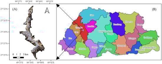
Figure 1. (A) Thimphu Thromde is the study area and the capital city of Bhutan. (B) A map of Bhutan, depicting the 20 Dzongkhags, one of which is Thimphu.

2. Materials and Methods

2.1. Data Acquisition and Processing

Table 1 provides the details on the various data used for this study.

Table 1. Required data and their sources and purposes.

Sl. No	Data	Source	Purpose
1	Landsat Images	Landsat Satellite/NASA	To determine the LULC, vegetation/built-up strength, and UHI
2	Boundary Map	Thromde Office	To demarcate the study area
3	Digital Elevation Model	SRTM/NASA	To determine the elevation

Landsat provides global coverage, with the Earth being divided into grids identifiable by their path and row numbers. Each grid has a swath area of 185 km × 180 km. Thimphu Thromde falls under the grid having the path and row numbers of 138/41. The data are in the form of multispectral images and as such are classified as raster data. Each pixel in the images represents an area of 30 m × 30 m on the actual ground. The satellite provides 11 different images, each measuring a different form of spectral wavelength [22]. The images are originally represented in the grayscale color, with the darker pixels representing areas that possess lower values of the wavelength and the lighter pixels having higher values. Analyzing the images makes it possible to conduct a whole host of different studies. For this study, the Landsat images were used to prepare maps that would detail the LULC, the vegetation biomass, the built-up strength, and the LST of the Thromde.

A Digital Elevation Model (DEM) was obtained from Shuttle Radar Topography Mission (SRTM). Similar to Landsat, SRTM provides global coverage with a spatial resolution of 30 m [23]. Although the DEM records multispectral wavelengths, SRTM uses imaging radar technology to record the elevation data. The DEM is also a raster form of data where each pixel is encoded with the elevation of the area in meters. The DEM was used to determine the elevation ranges of the Thromde and its variation with the UHI. The DEM was also used to delineate the water bodies of the Thromde to study its variation with the UHI.

An imperative prerequisite when working with remote sensing data is data cleaning. When the sensors are onboard, the satellite records the spectral wavelength, and there can be some minor errors due to the presence of the atmosphere. Certain portions of the light may undergo scattering/refraction or absorption, which can affect the readings. The absorption of light reduces the intensity, whereas scattering can cause the values of neighboring pixels to crossover with each other. The atmospheric correction was performed using the correction algorithm given by Equation (1) [24]:

TOA = M_L × Q_cal × A_L

(1)

where TOA denotes the spectral radiance, M_L denotes the band-specific multiplicative rescaling factor, Q_cal denotes the calibrated quantization value of the pixel, and A_L denotes the band-specific additive scaling factor. The values of M_L, Q_cal, and A_L are all specified in the metadata file that is provided along with the Landsat data.

2.2. Methodology

The required data such as the multispectral images from the Landsat satellite, a Digital Elevation Model of the Thromde, and the boundary map of the study area were obtained. The Landsat images of November 2001 and 2021 were acquired, and the data were cleaned to conduct the atmospheric corrections. After the data were cleaned, the land use and land cover of the Thromde were mapped.

The LST of the Thromde was then determined using the Landsat data. The LST was used to determine the presence of the UHI for 2001 and 2021 and to study the variations in the UHI in the last two decades. The LULC and UHI maps were then used for the simulation using Artificial Neural Networks. The LST maps were validated using the field measurements of the surface temperature. The LULC maps were validated through land class comparison using Google Earth images and field visits. The simulation model was validated by preparing a LULC simulation for 2021 and comparing it with the actual LULC map (Figure 2).

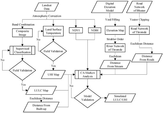
Figure 2. The research methodology.

2.3. Land Use and Land Cover Modeling

Land use and land cover (LULC) maps depict the biophysical properties of a study area. These maps generally quantify the spatial coverage of the different forms of land classes such as the amount of built-up land, vegetative areas, barren land, water bodies, and other such physical properties of the Earth’s surface. Two LULC maps for the years 2001 and 2021 were prepared to understand the spatial variations in the study area’s land cover.

Using the Landsat data, a composite image of the Thromde was prepared. Composite images depict the natural colors of an area, instead of the usual grayscale color of the Landsat images. These images are the actual representations of how the Earth’s surface appears when viewed from space.

To create the composite image, the Landsat bands 2, 3, and 4 were combined. These bands represent the blue, green, and red colors, respectively. The combination of these primary colors results in the creation of a natural color image. The study area portion was demarcated and extracted using the Thromde’s boundary map.

Using the composite image, a supervised classification, machine learning model was trained to differentiate between four different forms of land classes, as detailed in Table 2.

Table 2. LULC class designation.

Sl. No	Class Name	Class Description
1	Built-up	Urban Settlements, Commercial Areas, Roads, Pavements, Parking, and Man-made structures
2	Vegetation	Forests, Agricultural Fields, Parks, Grasslands, and Meadows
3	Barren	Sand, Gravel, Rocks, and River Banks
4	Water	Rivers, Lakes, and Streams

2.4. Determination of LST

The Normalized Difference Vegetation Index (NDVI) map is the most commonly used index for studying the vegetative biomass of an area [25,26] (Equation (2)):

$$\mathrm{NDVI} = {\displaystyle \frac{\mathrm{NIR} - \mathrm{Red}}{\mathrm{NIR} + \mathrm{Red}}}$$

(2)

where NIR represents the Landsat Near-Infrared Band, and RED represents the Landsat Red Band.

The Normalized Difference Built-up Index (NDBI) was used to quantify the built-up content of the Thromde, using the algorithm (Equation (3)) [27]:

$$\mathrm{NDBI} = {\displaystyle \frac{\mathrm{SWIR} - \mathrm{NIR}}{\mathrm{SWIR} + \mathrm{NIR}}}$$

(3)

where SWIR denotes the Shortwave Infrared Band, and NIR denotes the Landsat Near-Infrared Band.

The LST of Thimphu Thromde was computed from the Landsat data using the following methodology [24]:

• Calculation of TOA spectral radiance:

The Landsat bands must be corrected for measurement errors due to the presence of the atmosphere. This was performed using Equation (1).

2.

Calculation of brightness temperature (BT) (Equation (4)):

$$\mathrm{BT} ={\displaystyle \frac{{\mathrm{K}}_2}{\ln \left(\frac{{\mathrm{K}}_1}{\mathrm{TOA}}\right)+1}} - 273.15$$

(4)

K₁ and K₂ denote conversion constants that are also specified in the metadata file. BT represents the brightness temperature that denotes the LST of the area.

3.

The proportion of vegetation (P_v):

P_v is the degree of vegetation coverage of the area and is calculated using Equation (5):

$$\mathrm{P}\mathrm{v} = \left({\displaystyle \frac{\mathrm{NDVI} - {\mathrm{NDVI}}_{\min }}{{\mathrm{NDVI}}_{\max } - {\mathrm{NDVI}}_{\min }}}\right)$$

(5)

NDVI_max and NDVI_min represent the maximum and minimum values of NDVI present in the NDVI map, respectively.

4.

Calculation of Emissivity (e):

Emissivity is the effectiveness of an area in emitting radiation. It is calculated from P_v as follows (Equation (6)):

$${\mathrm{e} = \mathrm{m} \times \mathrm{P}}_{\mathrm{v}} + \mathrm{n}$$

(6)

where m is 0.004 [28] and n is 0.986 [28]; they are the emissivity constants and are obtained from the Landsat metadata file.

5.

The LST:

Upon obtaining the value of e, BT can be corrected to obtain the LST as follows (Equation (7)):

$$\mathrm{LST} = {\displaystyle \frac{\mathrm{BT}}{1+\mathrm{w}(\frac{\mathrm{BT}}{{\mathrm{P}}_{\mathrm{v}}})\times \ln \left(\mathrm{e}\right)}}$$

(7)

The spectral wavelength, w, is specified within the Landsat data.

2.5. Mapping of UHIs

The UHIs were then identified and demarcated. This was performed by normalizing the LST map to make the presence of UHIs more identifiable. The normalization method is specified in Table 3.

Table 3. The temperature class ranges used to normalize the LST.

Sl. No	Class Name	Class Range
1	Very Cold	T ≤ (μ − 1.5σ)
2	Cold	(μ − 1.5σ) < T < (μ − σ)
3	Moderate	(μ − σ) < T < (μ + σ)
4	Hot	(μ + σ) < T < (μ + 1.5σ)
5	Very Hot	T ≥ (μ + 1.5σ)

T denotes the LST of the individual pixels, μ denotes the mean LST, and σ denotes the standard deviation.

2.6. Simulation of LULCs and UHIs

After determining the variations in the LULC, a simulation study was conducted to predict the spatial conditions of the Thromde for 2031. The CA-Markov model was executed for the simulation. This model considers multiple spatial factors associated with the LULC/UHI for different periods. The factors considered in the simulation were vegetation content, built-up content, the elevation of the Thromde, and distances from roads, built-up structures, and streams. Then, it executes an algorithm, which predicts the future spatial conditions.

The algorithm (Equation (8)) is mathematically represented as follows [29]:

$${\mathrm{S}}_{(\mathrm{t},\mathrm{t}+1)} = {\mathrm{P}}_{\mathrm{ij} }\times \mathrm{S}\left(\mathrm{t}\right)$$

(8)

$${\mathrm{P}}_{\mathrm{ij}}=\left[\begin{array}{cccc}{\mathrm{P}}_{11}& {\mathrm{P}}_{12}& \cdots & {\mathrm{P}}_{1\mathrm{n}}\\ {\mathrm{P}}_{21}& {\mathrm{P}}_{21}& \cdots & {\mathrm{P}}_{2\mathrm{n}}\\ ⋮& ⋮& & ⋮\\ {\mathrm{P}}_{\mathrm{n}1}& {\mathrm{P}}_{\mathrm{n}2}& \cdots & {\mathrm{P}}_{\mathrm{nn}}\end{array}\right]$$

where S_t represents the state of the system at time t, S_t+1 represents the state of the system at time t + 1, P represents the transition probability, and P_ij represents the transition probability matrix.

2.7. Accuracy Assessment of LULCs

After the preparation of the maps, their accuracy had to be assessed to validate the findings. This was performed by comparing the land classes specified by the LULC maps with the actual land classes in the field. Multiple points on the LULC maps were randomly selected, and their coordinates were recorded. The coordinates were input into Google Earth Pro, and the land classifications based on their satellite images were noted down. A comparison between the LULC land classes and the high-resolution images of the Thromde from Google Earth images was conducted to obtain the accuracy in terms of total correctly predicted land classifications.

2.8. Field Verification of LST

To validate the accuracy of the LST map obtained from the Landsat data, the field measurement of the Thromde’s LST was carried out. This was performed by selecting random locations in the Thromde and measuring their LSTs. The measurement was conducted on the exact day and time as those shown in the Figure 3.

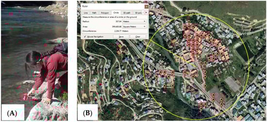
Figure 3. Field validation of Landsat LST by (A) conducting the field measurements of LST using an infrared thermometer for an area of (B) 400,000 m², encompassing more than 100 points.

An infrared thermometer with a measuring range of −50 °C~500 °C (−58 °F~932 °F), an accuracy of ±1.5 °C/±1.5%, and a resolution of 0.1 °C or 0.1 °F was used to conduct the field measurements of the LST. The field measurement of the LST was collected and compared with the Landsat LST using the Root Mean Square Error (RMSE).

3. Results

3.1. LULC of the Thromde

Based on the supervised classification model, the LULC maps for 2001 and 2021 (Figure 4) were prepared. The four classes differentiated by the model were color-coded for demarcation. Table 4 provides the details of the total land coverage of the different classes.

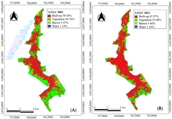
Figure 4. LULC class details for (A) 2001 and (B) 2021. The two maps were colored following the same color coding for an easier comparison between the two.

Table 4. LULC class details for 2001 and 2021.

Class	LULC Classification 2001		LULC Classification 2021
	Area (km2)	Percentage Area	Area (km2)	Percentage Area
Built-up	13.24	50.58	17.69	67.57
Vegetation	11.72	44.76	6.65	25.4
Barren	0.91	3.47	1.48	5.66
Water	0.31	1.19	0.36	1.36

3.2. LST of the Thromde

Figure 5 shows the spatial distribution of LST in Thimphu Thromde for the year 2001 and 2021. The figure shows a clear increase in the LST over time with higher LST values and a wider a extent of the high temperature zones. The figure indicates an intensification in the surfacing warming taking place in the study area.

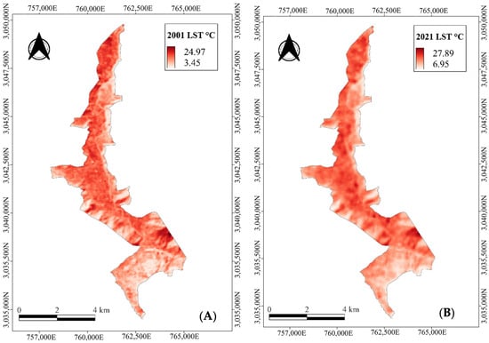
Figure 5. The LST map for the years (A) 2001 and (B) 2021. The LST has been color-coded in a white-red gradient, with higher temperatures depicted using a redder color.

3.3. UHI of the Thromde

From the LST maps (Figure 6), the surface temperatures of the Thromde were normalized to make the distinction between the relatively hotter zones more observable. Table 5 provides the details of the UHI classification of the Thromde.

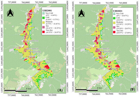
Figure 6. The UHI maps for the years (A) 2001 and (B) 2021.

Table 5. UHI details for 2021.

Class	Area (km2)	Percentage Area
Very Cold	2.18	8.32
Cold	2.80	10.68
Moderate	17.00	64.95
Hot	3.10	11.83
Very Hot	1.10	4.22

3.4. LULCs—UHIs Simulation Results

The ANN process is shown in Figure 7. The input layers were the factors affecting the LULC and UHI. The analysis of the data was executed in the hidden layer, and the output layer was the final LULC prediction.

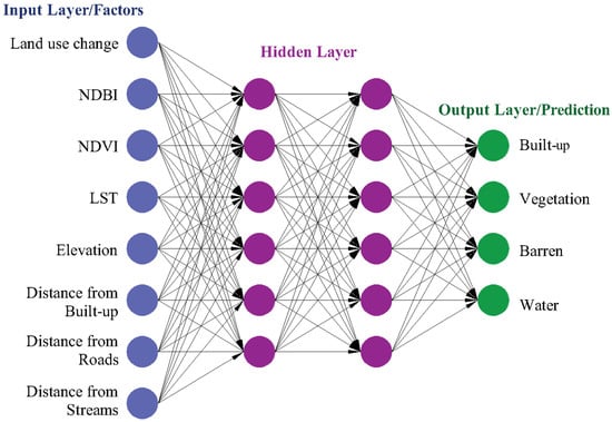
Figure 7. Graphical representation of the ANN architecture. The input layer that is colored blue is the factor that affects the LULC and UHI. The ANN analysis is conducted in the hidden layer. The output layer that is colored in green is the final output of the ANN algorithm.

The LULC and UHI maps (Figure 8) were then used to simulate the spatial conditions for 2031 along with other factors such as built-up content, the elevation of the Thromde, and distances from roads, built-up structures, and streams.

Figure 8. Simulation results for (A) LULC 2031 using an ANN. The map details the individual class changes in the Thromde’s land cover. (B) UHI for 2031. The simulated UHI map details the location and the potential changes in the total areal coverage of UHI and non-UHI zones.

4. Accuracy Assessment

4.1. Accuracy of LULCs

To assess the accuracy of the 2021 LULC map, high-resolution images from Google Earth Pro were used. A total of 160 random points on the LULC maps were selected based on Table 6 [30].

Table 6. Sample size distribution.

Sl. No	Class	Ratio	Sample Size
1	Built-up	4	4/10 × 160 = 64
2	Vegetation	3	3/10 × 160 = 48
3	Barren	2	2/10 × 160 = 32
4	Water	1	1/10 × 160 = 16
		Total Samples:	160

The LULC classifications of the points were noted and then compared with the actual classification observed from the Google Earth Pro images. An accuracy of 80.48% was obtained.

4.2. Field Validation Results of LST

An infrared thermometer was used to conduct the field measurements of the LST. The coordinates of the points were recorded, and the field LST was compared with the Landsat LST. A graph showing the correlation between the two forms of measurements was prepared (Figure 9). The RMSE obtained was 2.9 °C, which was similar to the RMSE values obtained by other researchers [13].

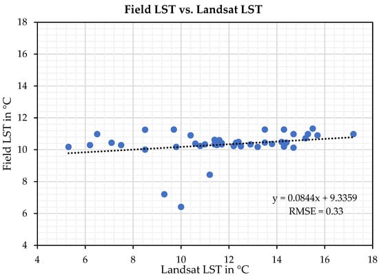
Figure 9. Field LST vs. Landsat LST.

4.3. Validation of Simulation Model

The accuracy assessment of prediction studies proved to be a challenge, as it is not possible to conduct field verification. However, many researchers have successfully predicted the LULC for their study areas using the CA-Markov model. Furthermore, this model was used to simulate the Thromde’s LULC for 2021 (Figure 10), and a comparison was made with the actual LULC.

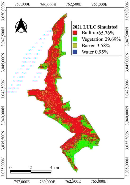
Figure 10. Simulated LULC for 2021 was compared with the actual LULC map prepared for 2021. When comparing the simulated and the actual LULC maps, an average class difference of 2.4% was observed.

5. Discussion

5.1. Transitions of the Thromde’s LULC

When comparing the two LULC maps prepared for the Thromde (Table 7), it was observed that, within the last two decades, the Thromde has undergone considerable urbanization. The built-up area had increased by 4.45 km² or by 16.99%. The vegetation cover had decreased by 5.07 km² or 19.36%. The lands classified as barren had increased by 0.57 km². The presence of water bodies had slightly increased by 0.05 km² or 0.17%.

Table 7. LULC transition from 2001 to 2021.

Class	Changes in Area (km2)
Built-up	4.45
Vegetation	−5.07
Barren	0.57
Water	0.05

5.2. LST of the Thromde

The LST of the Thromde, determined from the Landsat satellite, shows considerable variation, based on the area’s location and land classification. From 2001 to 2021, the difference between the maximum and minimum LST computed for the study area ranged from 18.33 °C to 25.74 °C, with the average difference being 20.74 °C. The higher ranges of the LST were disproportionately located more in the urban towns. It was observed that, even within the towns themselves, there were variations in the temperature. The maximum temperatures calculated for 2001 and 2021 were all located in core urban towns where built-up areas were predominant. These areas with the highest intensity of LST consisted of large multistory buildings, pavements, and roads where heavy traffic and other forms of built-up content were present. It was also observed that, if a built-up area had slightly more vegetation, such as trees along the footpaths, the LST of this area was a few degrees lower compared to other built-up areas in close proximity.

5.3. Presence of UHIs

The LST map prepared for the Thromde had large variations in the intensity of the surface temperature. The lowest LST was 6.95 °C, and the highest LST was 27.89 °C. The LST map was normalized for clearer visualization of the variations in LST. From the normalized LST map, it was observed that there were many instances of UHIs present within the thromde. Some regions had temperature differences of about 6.92 °C, when compared with the surrounding LST. All the UHIs were located in regions classified as urban. With the help of satellite images and field visits, it was determined that the heat islands were located in the core metropolitan areas, mostly made up of high-rise buildings and asphalt pavements.

The places most susceptible to the UHI effect were identified from the UHI maps. Popular landmarks such as Jigme Dorji Wangchuk National Referral Hospital and the Thimphu Clock Tower are classified as extreme UHI zones. The core residential towns like Motithang and commercial hubs like Tashi Commercial are also classified as extreme UHIs. It was observed that places where built-up areas such as multistory structures and pavements were prominent were likely to be classified as UHI zones. Artificial football turfs also seem to be a major contributor to UHIs as around eleven turfs were located, all of which were classified as UHI zones. Even large barren lands with minimal built-up structures were part of moderate UHI zones and were determined to be UHI formation contributors.

5.4. Simulated LULC for 2031

Similar to past trends, the LULC simulation results (Table 8) predict that significant changes in the land cover of the Thromde will occur due to the built-up area replacing the vegetative and barren land. From the simulated map, it was observed that most of the increase in built-up content is predicted to take place in areas in close proximity or on the outskirts of the pre-existing towns. This suggests that the increase in built-up areas in the next decade will be due to urban sprawl and the expansion of the urban area.

Table 8. Predicted LULC class coverage for 2021 vs. 2031.

Sl. No	Class	2021 Coverage %	2031 Coverage %	Changes
1	Built-up	67.57	72.82	5.25
2	Vegetation	25.4	23.52	−1.88
3	Barren	5.66	3.28	−2.38
4	Water	1.36	0.38	−0.98

5.5. Simulated UHI for 2031

In accordance with the increase in the built-up content predicted by the simulated LULC maps, the UHI condition of the Thromde is also projected to worsen. Upon comparing the present and the future UHI conditions (Table 9), the areas classified as hot and very hot UHIs are predicted to increase to 14.27% (3.73 km²) and 6.09% (1.59 km²) of the total Thromde area, respectively.

Table 9. Future transition of the UHI condition.

Class	2021		2031
	Area (km2)	Percentage	Area (km2)	Percentage
Very Cold	2.18	8.32	2.18	8.31
Cold	2.80	10.68	2.90	11.07
Moderate	17.00	64.95	15.77	60.26
Hot	3.10	11.83	3.73	14.27
Very Hot	1.10	4.22	1.59	6.09

6. Conclusions

The presence and intensity of UHIs were evaluated using multispectral Landsat satellite imagery and a Digital Elevation Model (DEM) from SRTM. The Landsat data were corrected for atmospheric errors, following which NDVI and NDBI maps were generated to evaluate vegetation biomass and to delineate built-up areas. These maps provided an initial understanding of the spatial characteristics of the study area. The LULC maps were subsequently prepared for the years 2001 and 2021 using the supervised classification of the Landsat data, enabling the quantification of built-up areas, vegetation, barren land, and water bodies. An analysis of class transitions revealed significant urban expansion over the last two decades. In 2021, the built-up area coverage was determined to be 67.57% and the vegetation cover to be 25.40%.

To determine the LST of the land classes present in the Thromde, the thermal band of the Landsat data was used, and the LST maps were prepared for 2001 and 2021. The UHIs of the Thromde were demarcated by classifying the temperatures based on their intensities in the LST maps.

A simulation of the LULC and UHI conditions for 2031 was carried out using the CA-Markov model. The modeling was carried out using key driving factors such as NDVI, NDBI, elevation, and distances from roads, built-up structures, and streams. The modeling results indicate a continued expansion of the urban area, with built-up areas projected to reach 72.82% and the vegetation coverage expected to reach 23.52% by the year 2031. Correspondingly, UHI zones classified as hot and very hot are expected to increase to 14.26% and 6.08% of the total thromde area, respectively.

Multiple validation methods were implemented to determine the accuracy of the results. To validate the LULC maps, multiple random points were selected on the maps, and their classifications were compared with the field classification. Field measurements were conducted to determine the accuracy of the Landsat LST. A simulation for the present scenario was conducted to verify the feasibility of the ANN model.

References

- Hassan, T.; Zhang, J.; Prodhan, F.A.; Pangali Sharma, T.P.; Bashir, B. Surface Urban Heat Islands Dynamics in Response to Lulc and Vegetation across South Asia (2000–2019). Remote Sens. 2021, 13, 3177. [Google Scholar] [CrossRef]
- Wang, S.W.; Munkhnasan, L.; Lee, W.K. Land Use and Land Cover Change Detection and Prediction in Bhutan’s High Altitude City of Thimphu, Using Cellular Automata and Markov Chain. Environ. Chall. 2021, 2, 100017. [Google Scholar] [CrossRef]
- Chen, L.; Jiang, R.; Xiang, W.N. Surface Heat Island in Shanghai and Its Relationship with Urban Development from 1989 to 2013. Adv. Meteorol. 2016, 2016, 9782686. [Google Scholar] [CrossRef]
- Rajeshwari, A. Estimation of Land Surface Temperature of Dindigul District Using Landsat 8 Data. Int. J. Res. Eng. Technol. 2014, 03, 122–126. [Google Scholar] [CrossRef]
- Swamy, G.; Shiva Nagendra, S.M.; Schlink, U. Urban Heat Island (UHI) Influence on Secondary Pollutant Formation in a Tropical Humid Environment. J. Air Waste Manag. Assoc. 2017, 67, 1080–1091. [Google Scholar] [CrossRef] [PubMed]
- Mohajerani, A.; Bakaric, J.; Jeffrey-Bailey, T. The Urban Heat Island Effect, Its Causes, and Mitigation, with Reference to the Thermal Properties of Asphalt Concrete. J. Environ. Manag. 2017, 197, 522–538. [Google Scholar] [CrossRef] [PubMed]
- Abdel-Ghany, A.M.; Al-Helal, I.M.; Shady, M.R. Human Thermal Comfort and Heat Stress in an Outdoor Urban Arid Environment: A Case Study. Adv. Meteorol. 2013, 2013, 693541. [Google Scholar] [CrossRef]
- Stalhandske, Z.; Nesa, V.; Zumwald, M.; Ragettli, M.S.; Galimshina, A.; Holthausen, N.; Röösli, M.; Bresch, D.N. Projected Impact of Heat on Mortality and Labour Productivity under Climate Change in Switzerland. Nat. Hazards Earth Syst. Sci. 2021, 22, 2531–2541. [Google Scholar] [CrossRef]
- O’Malley, C.; Piroozfarb, P.A.E.; Farr, E.R.P.; Gates, J. An Investigation into Minimizing Urban Heat Island (UHI) Effects: A UK Perspective. Energy Procedia 2014, 62, 72–80. [Google Scholar] [CrossRef]
- Leal Filho, W.; Wolf, F.; Castro-Díaz, R.; Li, C.; Ojeh, V.N.; Gutiérrez, N.; Nagy, G.J.; Savić, S.; Natenzon, C.E.; Al-Amin, A.Q.; et al. Addressing the Urban Heat Islands Effect: A Cross-Country Assessment of the Role of Green Infrastructure. Sustainability 2021, 13, 753. [Google Scholar] [CrossRef]
- Keppas, S.C.; Papadogiannaki, S.; Parliari, D.; Kontos, S.; Poupkou, A.; Tzoumaka, P.; Kelessis, A.; Zanis, P.; Casasanta, G.; De’donato, F.; et al. Future Climate Change Impact on Urban Heat Island in Two Mediterranean Cities Based on High-Resolution Regional Climate Simulations. Atmosphere 2021, 12, 884. [Google Scholar] [CrossRef]
- Mirzaei, P.A.; Haghighat, F. Approaches to Study Urban Heat Island—Abilities and Limitations. Build. Environ. 2010, 45, 2192–2201. [Google Scholar] [CrossRef]
- Mejbel Salih, M.; Zakariya Jasim, O.; Hassoon, K.I.; Jameel Abdalkadhum, A. Land Surface Temperature Retrieval from LANDSAT-8 Ther-Mal Infrared Sensor Data and Validation with Infrared Ther-Mometer Camera. Int. J. Eng. Technol. 2018, 7, 608–612. [Google Scholar] [CrossRef]
- Szymanowski, M.; Kryza, M. GIS-Based Techniques for Urban Heat Island Spatialization. Clim. Res. 2009, 38, 171–187. [Google Scholar] [CrossRef]
- Ma, W.; Feng, Z.; Cheng, Z.; Chen, S.; Wang, F. Identifying Forest Fire Driving Factors and Related Impacts in China Using Random Forest Algorithm. Forests 2020, 11, 507. [Google Scholar] [CrossRef]
- Nguyen, T.T. Landsat Time-Series Images-Based Urban Heat Island Analysis: The Effects of Changes in Vegetation and Built-up Land on Land Surface Temperature in Summer in the Hanoi Metropolitan Area, Vietnam. Environ. Nat. Resour. J. 2020, 18, 177–190. [Google Scholar] [CrossRef]
- Weng, Q.; Fu, P.; Gao, F. Generating Daily Land Surface Temperature at Landsat Resolution by Fusing Landsat and MODIS Data. Remote Sens. Environ. 2014, 145, 55–67. [Google Scholar] [CrossRef]
- Wulder, M.A.; Loveland, T.R.; Roy, D.P.; Crawford, C.J.; Masek, J.G.; Woodcock, C.E.; Allen, R.G.; Anderson, M.C.; Belward, A.S.; Cohen, W.B.; et al. Current Status of Landsat Program, Science, and Applications. Remote Sens. Environ. 2019, 225, 127–147. [Google Scholar] [CrossRef]
- Roy, D.P.; Wulder, M.A.; Loveland, T.R.; Woodcock, C.E.; Allen, R.G.; Anderson, M.C.; Helder, D.; Irons, J.R.; Johnson, D.M.; Kennedy, R.; et al. Landsat-8: Science and Product Vision for Terrestrial Global Change Research. Remote Sens. Environ. 2014, 145, 154–172. [Google Scholar] [CrossRef]
- Liping, C.; Yujun, S.; Saeed, S. Monitoring and Predicting Land Use and Land Cover Changes Using Remote Sensing and GIS Techniques- A Case Study of a Hilly Area, Jiangle, China. PLoS ONE 2018, 13, e0200493. [Google Scholar] [CrossRef]
- Liu, C.; Li, Y. Spatio-Temporal Features of Urban Heat Island and Its Relationship with Land Use/Cover in Mountainous City: A Case Study in Chongqing. Sustainability 2018, 10, 1943. [Google Scholar] [CrossRef]
- Traore, M.; Lee, M.S.; Rasul, A.; Balew, A. Assessment of Land Use/Land Cover Changes and Their Impacts on Land Surface Temperature in Bangui (the Capital of Central African Republic). Environ. Chall. 2021, 4, 100114. [Google Scholar] [CrossRef]
- Elkhrachy, I. Vertical Accuracy Assessment for SRTM and ASTER Digital Elevation Models: A Case Study of Najran City, Saudi Arabia. Ain Shams Eng. J. 2018, 9, 1807–1817. [Google Scholar] [CrossRef]
- Rosado, R.M.G.; Guzmán, E.M.A.; Lopez, C.J.E.; Molina, W.M.; Garciá, H.L.C.; Yedra, E.L. Mapping the LST (Land Surface Temperature) with Satellite Information and Software ArcGis. IOP Conf. Ser. Mater. Sci. Eng. 2020, 811, 012045. [Google Scholar] [CrossRef]
- Jiang, Z.; Huete, A.R.; Chen, J.; Chen, Y.; Li, J.; Yan, G.; Zhang, X. Analysis of NDVI and Scaled Difference Vegetation Index Retrievals of Vegetation Fraction. Remote Sens. Environ. 2006, 101, 366–378. [Google Scholar] [CrossRef]
- Zaitunah, A.; Samsuri, S.; Ahmad, A.G.; Safitri, R.A. Normalized Difference Vegetation Index (Ndvi) Analysis for Land Cover Types Using Landsat 8 Oli in Besitang Watershed, Indonesia. IOP Conf. Ser. Earth Environ. Sci. 2018, 126, 012112. [Google Scholar] [CrossRef]
- Rakib, A.A.; Akter, K.S.; Rahman, N.; Arpi, S.; Kafy, A. Analyzing the Pattern of Land Use Land Cover Change and Its Impact on Land Surface Temperature: A Remote Sensing Approach. In Proceedings of the 1st International Student Research Conference, Dhaka, Bangladesh, 6 December 2020; pp. 1–11. [Google Scholar]
- Mansourmoghaddam, M.; Rousta, I.; Cabral, P.; Ali, A.A.; Olafsson, H.; Zhang, H.; Krzyszczak, J. Investigation and Prediction of the Land Use/Land Cover (LU/LC) and Land Surface Temperature (LST) Changes for Mashhad City in Iran during 1990–2030. Atmosphere 2023, 14, 741. [Google Scholar] [CrossRef]
- Tadese, S.; Soromessa, T.; Bekele, T. Analysis of the Current and Future Prediction of Land Use/Land Cover Change Using Remote Sensing and the CA-Markov Model in Majang Forest Biosphere Reserves of Gambella, Southwestern Ethiopia. Sci. World J. 2021, 2021, 6685045. [Google Scholar] [CrossRef]
- Chimi, C.; Tenzin, J.; Cheki, T. Assessment of Land Use/Cover Change and Urban Expansion Using Remote Sensing and GIS: A Case Study in Phuentsholing Municipality, Chukha, Bhutan. Int. J. Energy Environ. Sci. 2017, 2, 127–135. [Google Scholar] [CrossRef]
Disclaimer/Publisher’s Note: The statements, opinions and data contained in all publications are solely those of the individual author(s) and contributor(s) and not of MDPI and/or the editor(s). MDPI and/or the editor(s) disclaim responsibility for any injury to people or property resulting from any ideas, methods, instructions or products referred to in the content. |
© 2025 by the authors. Licensee MDPI, Basel, Switzerland. This article is an open access article distributed under the terms and conditions of the Creative Commons Attribution (CC BY) license (https://creativecommons.org/licenses/by/4.0/).