Enhancing Forecasting Capabilities Through Data Assimilation: Investigating the Core Role of WRF 4D-Var in Multidimensional Meteorological Fields

Abstract

As climate change intensifies, enhancing numerical weather prediction (NWP) accuracy has been increasingly critical. While data assimilation optimizes NWP initial conditions, its effectiveness over complex terrain requires further systematic evaluation. This study implemented a high-resolution WRF/4D-Var data assimilation framework, overcoming its inherent limitation of not supporting two-layer nested assimilation across domains by designing a two-layer nested “assimilation-forecast” workflow. Representative winter and summer cases from February and June 2019 were selected to evaluate improvements in near-surface and upper-air meteorological parameters. The results indicated that the 4D-Var data assimilation significantly improved the correlation coefficients of near-surface variables during winter by 2.9% (temperature), 14.5% (relative humidity), 6.6% (wind speed), and 10.4% (wind direction), with even greater improvements observed in summer reaching 13.3%, 5.8%, 35.3%, and 42.3%, respectively. Meanwhile, 4D-Var considerably enhanced the atmospheric vertical profiling, with the middle troposphere (300–700 hPa) exhibiting the most pronounced improvement. Among different surface types, water bodies exhibited the strongest assimilation response. Results also revealed systematic corrections to the background fields, with February exhibiting more uniform adjustments in contrast to June’s complex spatiotemporal patterns. Positive effects persisted throughout the 24-h forecasts, with the maximum benefit occurring within the first 12 h. These results demonstrate the effectiveness of 4D-Var in regional meteorological forecasting, highlighting its value for constructing high-precision multidimensional meteorological fields to support both weather and air quality simulations.

1. Introduction

Numerical Weather Prediction (NWP), as the core technology of modern meteorological forecasting, plays an indispensable role in weather and climate prediction as well as atmospheric environmental research. Despite its importance, the forecast accuracy is often constrained by multiple factors, such as uncertainties in the initial conditions, limitations of the parameterization schemes for physical processes, and scale effects arising from insufficient model resolution [1,2]. Among them, the quality of the initial conditions is recognized as the decisive factor affecting the accuracy of numerical forecasts [3,4]. As the starting point of numerical integration, the initial atmospheric state must not only incorporate clear large-scale circulation information but also fully reflect the mesoscale features that trigger significant weather processes. Any deficiencies or uncertainties in the background fields can quickly amplify during model integration, degrading forecast skill. Given that atmospheric observations are characterized by uneven spatial distribution, coarse temporal resolution, and inherent errors, the construction of high-quality initial conditions poses a major challenge in numerical weather prediction research.

Data assimilation, as a systematic methodology, effectively improves model initial conditions by organically combining observational information with the model background field, thereby enhancing forecast accuracy [5,6,7]. Numerous studies have confirmed the positive impact of data assimilation on improving forecasting skill. At the global scale, major operational centers such as the European Centre for Medium-Range Weather Forecasts (ECMWF) [8,9,10,11,12,13], the National Centers for Environmental Prediction (NCEP) [14,15] and the Japan Meteorological Agency (JMA) [16,17] have implemented advanced data assimilation systems to assimilate multi-source observations, significantly enhancing the accuracy of medium- to long-range weather forecasts. Currently, data assimilation methods can be broadly divided into two categories: variational methods and ensemble-based statistical methods. Among them, 4D-Var as an advanced form of variational assimilation, not only simultaneously accounts for the error characteristics of observations and the background but also maintains spatiotemporal consistency under the dynamical constraints of the model within the assimilation window. Consequently, it has been widely adopted in operational NWP [18,19].

Compared to 3D-Var, 4D-Var can more effectively utilize asynchronous observations and achieve optimal estimation of the background field through the synergistic interaction of forward, tangential, and adjoint models [20,21]. Vourlioti et al. [22] employed 4D-Var to blend surface station data and the Integrated Multi-satellitE Retrievals for Global Precipitation Measurement (IMERG) satellite precipitation product with background fields from the Global Forecast System (GFS), using the result as improved initial conditions for prediction. The study revealed that 4D-Var assimilation benefited the temperature field throughout the forecast horizon. Xu et al. [23] directly assimilated hourly precipitation using 4D-Var and demonstrated that assimilation improved precipitation forecast accuracy and, to some extent, enhanced quantitative precipitation prediction skill. Yang et al. [24], through additional validation on multiple convective precipitation cases, confirmed that 4D-Var effectively adjusts the atmospheric thermodynamic structure, shortens model spin-up time, and improves short-range precipitation forecasts. In addition, studies on complex weather systems indicate that assimilating radar observations can effectively improve forecasts of severe convective weather [25,26,27].

Despite significant progress in existing research [28,29,30], the current literature remains limited in the systematicity and depth of its assessments of assimilation benefits. On the one hand, existing research has primarily focused on specific weather cases or single seasons [31,32,33,34,35], lacking systematic examination across weather backgrounds and seasons. Furthermore, previous work has neglected the spatial variation of assimilation benefits across different underlying surface types, limiting a comprehensive understanding of assimilation system performance under complex conditions. On the other hand, in-depth analysis of assimilation improvement mechanisms remains inadequate. Evaluations often focus on single meteorological variables [36], while key scientific questions—such as the synergistic improvement of multiple variables and their physical consistency, the intrinsic relationship between background field adjustment and forecast improvement, and the decay patterns of assimilation benefits with forecast lead time—have not been sufficiently explored.

In this study, we conducted a systematic assessment of the WRF 4D-Var system’s performance across different meteorological variables, seasons, and underlying surface conditions. This aims to address the limitations of previous studies regarding inter-seasonal, multi-parameter collaborative improvement assessments. We delve into the spatial heterogeneity of assimilation benefits and their correlation with underlying surface types, further clarifying the spatial correspondence between background field adjustments and forecast improvements, as well as the evolution of assimilation benefits over forecast lead times. Such assessments not only elucidate the strengths and weaknesses of the assimilation system but also provide scientific guidance for optimizing assimilation strategies and enhancing regional NWP capability.

2. Data and Methodology

2.1. Study Area and Time Period

Figure 1 depicts the topographical profile and regional configuration of the study area. To better capture detailed variations in local meteorological variables, we designed two-layer nested domains within the modeling system. As shown in Figure 1a, domain 1 covers most of China with a horizontal resolution of 27 km × 27 km, while domain 2 targets eastern China with a fine resolution of 9 km × 9 km. Two simulation periods in February and June 2019 were selected to represent mesoscale weather processes under different seasonal backgrounds. The figure also indicates the specific locations of near-surface and upper-air monitoring stations utilized for model evaluation (Figure 1b). The spatial distribution of underlying surface types is shown in Figure 1c, where the color bar corresponds to the numerical LU_INDEX (Land Use Index) values extracted directly from the WRF model’s static data, and lists the specific classifications of the underlying surface types included in this study area.

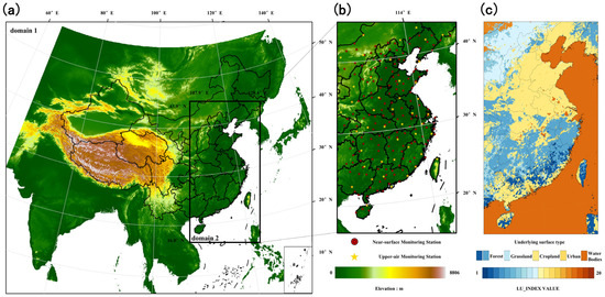
Figure 1. Sketch map of the study area: (a) the two-layer nested domains and the terrain elevation (m); (b) the distribution of near-surface and upper-air monitoring stations within domain 2; (c) the spatial distribution of underlying surface types, with the color bar indicating the corresponding LU_INDEX value.

2.2. Model Configuration

This study employed the regional numerical model WRF v4.6 and the four-dimensional variational assimilation system in WRF Data Assimilation, namely WRF 4D-Var v4.6, to construct the experimental framework. The 4D-Var method operates by combining the discrepancies between observations and the model background field over a given time window and incorporating them into a cost function $J\left({\mathbf{x}}_0\right)$ defined as follows:

$$\begin{array}{c}J\left({\mathbf{x}}_0\right)={\displaystyle \frac{1}{2}}{\left({\mathbf{x}}_0-{\mathbf{x}}_{\mathrm{b}}\right)}^{\mathrm{T}}{\mathbf{B}}^{-1}\left({\mathbf{x}}_0-{\mathbf{x}}_{\mathrm{b}}\right)+{\displaystyle \frac{1}{2}}{\displaystyle \sum _{t\in W}}{[{\mathbf{H}}_t{\mathbf{M}}_{0\to t}{\mathbf{x}}_0-{\mathbf{y}}_t]}^{\mathrm{T}}{\mathbf{R}}_t^{-1}\left[{\mathbf{H}}_t{\mathbf{M}}_{0\to t}{\mathbf{x}}_0-{\mathbf{y}}_t\right]\end{array}$$

(1)

where ${\mathbf{x}}_0$ denotes the initial state vector; ${\mathbf{x}}_{\mathrm{b}}$ is the background field vector; $\mathbf{B}$ is the background error covariance matrix; $W$ denotes the assimilation time window; ${\mathbf{H}}_t$ is the time-varying observation operator, which transforms the model state at time t into the model’s estimated observation value, placing it in the same space as the actual observation ${\mathbf{y}}_t$; ${\mathbf{M}}_{0\to t}$ is the WRF nonlinear model operator integrated from the initialization time to t, whose tangent linear model (TLM) and adjoint model (ADJ) are used for gradient computation; ${\mathbf{y}}_t$ is the observation field vector; ${\mathbf{R}}_t$ is the observation error covariance matrix.

The gradient is efficiently obtained using the adjoint model, and the minimization employs iterative optimization algorithms such as the conjugate gradient method. It is typically combined with multiple outer loops for linearization updates and several inner loop iterations. Throughout the assimilation process, it adjusts the model’s initial state and optimizes the variables at the initial time of the model to find the state that minimizes the cost function value, while constraining consistency with the background field. This yields the optimal initial state at the start time, ensuring that the model’s forecast within the entire assimilation window is most consistent with the observed data. Compared with 3D-Var, 4D-Var explicitly utilizes the temporal information of observations, thus enabling better handling of asynchronous observations and ensuring temporal consistency of the analysis.

Throughout the simulations, cyclic assimilation and forecast experiments were conducted by continuously ingesting real observations. The observed datasets were drawn from the NCEP ADP global upper air and surface weather observations [37], which integrates multiple sources of routine global surface and upper-air observations (e.g., SYNOP/METAR, SHIP/BUOY, TEMP/RAOB, AIREP/AMDAR) and can simultaneously be assimilated within a single assimilation window to incorporate both surface and upper-air observations.

The initial and lateral boundary conditions for WRF were provided by the ECMWF ERA5 reanalysis at 0.25° × 0.25° horizontal resolution and hourly temporal resolution, obtained from the Copernicus Climate Data Store (CDS) [38,39]. The model configuration employed 35 vertical levels with the top fixed at 50 hPa and a dynamic core with the non-hydrostatic framework. The primary physics options in WRF included the Thompson microphysics scheme [40], the Kain–Fritsch cumulus parameterization scheme [41], the Rapid Radiative Transfer Model for General Circulation Models Applications (RRTMG) longwave and shortwave radiation schemes [42], the Yonsei University (YSU) planetary boundary layer scheme [43], and the Noah Land-Surface scheme [44].

This experiment is designed as a day-cycled analysis and forecasting scheme, as illustrated in Figure 2. Each day begins with a 6-h WRF 4D-Var assimilation window from 00:00 to 06:00 UTC, which assimilates all available observations to produce an optimized analysis field valid at 00:00 UTC. This analysis serves as the deterministic initial condition to drive the standard WRF model for a 24-h forecast. The output (wrfout) constitutes the final simulation result for that day. Except for the initial run, the system employs a “warm-start” mechanism for cyclic coupling: the previous day’s 24-h forecast results serve as the first guess for the current day’s assimilation process. This “6-h analysis to 24-h forecast” cycle repeats daily throughout the one-month simulation period.

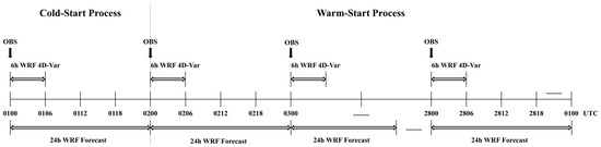
Figure 2. Cyclic Assimilation Process.

Additionally, this study innovatively employs a two-layer nested “assimilation-forecasting” workflow to achieve staged optimization from large to small scales. Since WRF 4D-Var inherently does not support cross-domain online bidirectional nested assimilation, we designed and implemented a cascading assimilation strategy to further focus on small-scale, local features and high-density observation areas, thereby significantly improving refined variables: 4D-Var assimilation is performed in both outer and inner domains to maximize utilization of local observations and high-resolution physical processes. The optimized analysis fields from both nested levels serve as initial conditions, enabling simultaneous initiation of nested-domain forecasts to enhance prediction quality.

The specific process is illustrated in Figure 3 below. First, assimilation is implemented in the coarse-grid parent domain (d01), applying multi-source observational constraints to the background field to correct initial errors in the large-scale circulation background. Subsequently, the ndown program transfers the analysis from d01 and its consistent boundary conditions within the assimilation window to the inner high-resolution domain (d02), constructing initial and boundary fields that align with the fine-grid dynamics and topographic details. Building upon this, d02 conducts a second-stage independent assimilation process, refining the initial state of local mesoscale and small-scale systems while maintaining large-scale consistency. Compared to traditional approaches implementing assimilation solely within a single domain or resolution, this strategy balances large-scale equilibrium with localized refinement. Ultimately, the optimized analysis fields from two-layer nested domains serve as consistent initial conditions, synchronously driving subsequent forecasting processes to significantly enhance overall forecasting capability.

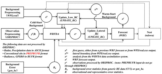
Figure 3. WRF 4D-Var components and workflow in nested simulations (solid boxes represent the standard single-domain process; dashed boxes indicate the extensions for the nested domain).

2.3. Model Evaluation

The performance of the WRF model in simulating two categories of meteorological variables—near-surface and upper-air—is evaluated by comparing hourly simulation data against observations, followed by an assessment with a series of statistical metrics. The near-surface meteorological parameters include: (1) temperature at 2 m, T₂; (2) relative humidity at 2 m, RH₂; (3) wind speed at 10 m, WS₁₀; and (4) wind direction at 10 m, WD₁₀. The observational data of these parameters were collected from the National Climate Data Center (NCDC), which is recorded mainly at 3 h intervals (with some 1 h sampling). The assessment of upper-air meteorological elements is conducted for meteorological parameters at different standard pressure levels (hPa), including: (1) temperature at 500 hPa, T₅₀₀; (2) relative humidity at 500 hPa, RH₅₀₀; (3) wind speed at 500 hPa, WS₅₀₀; and (4) wind direction at 500 hPa, WD₅₀₀. The observational data were sourced from the University of Wyoming’s 12 h resolution radiosonde dataset. The monitoring stations required for the aforementioned evaluations were uniformly distributed throughout the study region.

We will comprehensively evaluate the model’s performance across multiple dimensions in subsequent analyses. First, we employ the Mean Absolute Error (MAE) and the Mean Bias (MB) to assess the absolute magnitude and direction of errors, respectively. MAE provides an intuitive measure of the average gap between predicted and observed values, where lower values indicate better performance. MB, on the other hand, helps determine whether the model exhibits systematic overestimation (positive values) or underestimation (negative values), with absolute values closer to zero indicating smaller systematic bias. Mean Fractional Bias (MFB, %) and Mean Fractional Error (MFE, %) further gauge the credibility of model simulations. Generally, a model’s performance goal is considered met if the MFB falls within ±30% and the MFE is below 50%. Performance is considered acceptable if the MFB is within ±60% and the MFE remains under 75% [45]. Additionally, we employ the Root Mean Square Error (RMSE) to quantify the overall discrepancy between predicted and actual values. This metric is particularly sensitive to large errors; a smaller RMSE indicates higher predictive accuracy. The correlation coefficient (R) measures the linear relationship between predicted and observed values. As R approaches 1, it indicates stronger capture of data variations by the model and more ideal simulation performance [46]. For wind direction calculations, to avoid direct angle processing, we convert wind direction into unit vectors on a two-dimensional plane for computation. Additionally, to quantify the optimization, we defined the average improvement rate. For scalars such as air temperature, relative humidity, and wind speed, this improvement rate is calculated based on RMSE and defined as RATE. It should be noted that simulation results inevitably exhibit biases, which may stem from inherent limitations of the meteorological model itself. The aforementioned statistical metrics are specifically expressed as follows:

$$\begin{array}{c}MAE={\displaystyle \frac{\sum _{i=1}^N\left|x_m-x_o\right|}{N}}\end{array}$$

(2)

$$\begin{array}{c} MB={\displaystyle \frac{\sum _{i=1}^N\left(x_m-x_o\right)}{N}}\end{array}$$

(3)

$$\begin{array}{c}MFB={\displaystyle \frac{2}{N}}{\displaystyle \sum _{i=1}^N}{\displaystyle \frac{x_m-x_o}{x_m+x_o}}\times 100\%\end{array}$$

(4)

$$\begin{array}{c}MFE={\displaystyle \frac{2}{N}}{\displaystyle \sum _{i=1}^N}{\displaystyle \frac{\left|x_m-x_o\right|}{\left(x_m+x_o\right)}}\times 100\%\end{array}$$

(5)

$$\begin{array}{c}RMSE=\sqrt{{\displaystyle \frac{1}{N}}{\displaystyle \sum _{i=1}^N}{\left(x_m-x_o\right)}^2}\end{array}$$

(6)

$$\begin{array}{c}RATE={\displaystyle \frac{1}{N}}{\displaystyle \sum _{i=1}^N}{\displaystyle \frac{{RMSE}_{\_CTRL}-{RMSE}_{\_WRFDA}}{{RMSE}_{\_CTRL}}}\times 100\%\end{array}$$

(7)

$$\begin{array}{c}\Delta RMSE={RMSE}_{\_CTRL}-{RMSE}_{\_WRFDA}\end{array}$$

(8)

$$\begin{array}{c} R={\displaystyle \frac{\sum _{i=1}^N\left(x_m-\overline{x_m}\right)\left(x_o-\overline{x_o}\right)}{\sqrt{\sum _{i=1}^N{\left(x_m-\overline{x_m}\right)}^2\sum _{i=1}^N{\left(x_o-\overline{x_o}\right)}^2}}}\end{array}$$

(9)

where $x_m$ is the model-estimated value at station i at hour j, $x_o$ is the observed value at station i at hour j, $\overline{x_m}$ is the mean model-estimated value across all stations and hours, $\overline{x_o}$ is the mean observed value across all stations and hours, ${RMSE}_{\_CTRL}$ denotes the root mean square error for the control experiment, ${RMSE}_{\_WRFDA}$ denotes the root mean square error for the assimilation experiment, while $\Delta RMSE$ quantifies the change in root mean square error, and $N$ is the total sample number of all simulations and observations compared.

3. Results and Discussion

3.1. Overall Improvement of Forecasts by Data Assimilation

3.1.1. Near-Surface Meteorological Variables

As data assimilation is a key approach for correcting the model background field in numerical simulations, its practical effectiveness in improving the accuracy of near-surface meteorological variables requires systematic evaluation. Specific statistical performance is summarised in Table 1. Compared to the Control Experiment (CTRL), which is a standard WRF run without data assimilation, the Assimilation Experiment (WRFDA) showed superior performance in most of the statistical metrics overall. Although theoretical studies indicate that the assimilation process can effectively merge observational and model information, in practice, different meteorological variables in complex regional weather forecasting exhibit varying responses to assimilation. Based on comparative analysis of simulations from the CTRL experiment and the WRFDA experiment for February and June 2019, this section conducts an evaluation against observational data for four major near-surface meteorological parameters.

Table 1. Performance statistics for T₂, RH₂, WS₁₀, and WD₁₀.

Statistic		February		June
		CTRL	WRFDA	CTRL	WRFDA
T2 (°C)	MAE	2.40	1.92	2.62	1.76
	MB	0.45	1.13	1.23	0.38
	MFB (%)	−6.15	−1.25	4.69	1.53
	MFE (%)	36.49	−6.85	10.48	7.43
	RMSE	3.25	2.62	3.48	2.25
	R	0.94	0.97	0.78	0.88
RH2 (%)	MAE	14.85	11.03	14.15	11.13
	MB	−7.51	−2.04	−8.89	−1.03
	MFB (%)	−9.71	−2.04	−15.21	−1.76
	MFE (%)	24.77	18.23	24.54	17.65
	R	0.69	0.79	0.73	0.77
WS10 (m/s)	MAE	1.47	1.39	1.83	1.70
	MB	0.75	0.69	1.14	0.95
	MFB (%)	27.58	25.02	35.23	30.49
	MFE (%)	53.21	50.77	55.22	54.15
	RMSE	1.78	1.73	2.31	2.09
	R	0.57	0.61	0.42	0.57
WD10 (degrees)	R	0.69	0.77	0.40	0.59

Bold values indicate the optimum performance per row.

Figure 4 shows the observed–simulated scatter density plots of meteorological variables for (a) February and (b) June, representing winter and summer, respectively. The figure uses color to represent the density distribution of data points within specific regions. The dashed black line (1:1 reference line) and solid red line (linear regression fit) are employed to assess system bias. The results indicate that temperature field forecasts were significantly improved after the introduction of data assimilation. In winter, the correlation coefficient for the T₂ increased from 0.941 to 0.968, and the regression slope rose from 0.971 to 0.982, reflecting better simulation-observation and reduced systematic bias. In summer, the improvement in T₂ was more pronounced, with the correlation coefficient increasing by 13.3%; the high-density core region, previously located below the reference line (indicating overestimation), shifted back toward the reference line, indicating a strong constraint of the assimilation system on the summer temperature field.

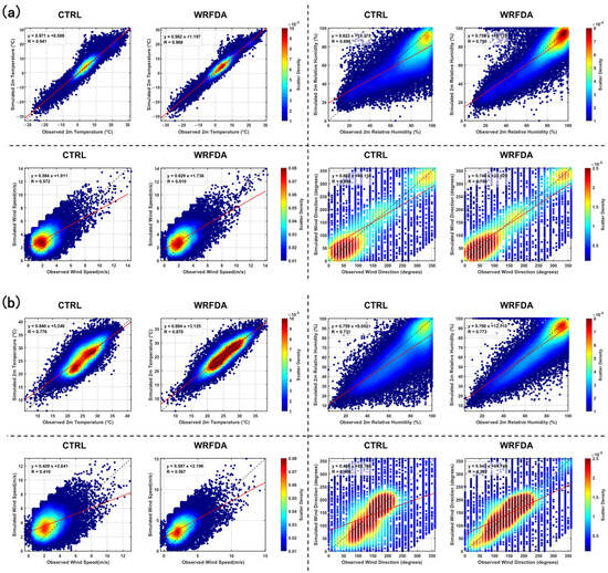
Figure 4. Comparisons of observed and simulated near-surface meteorological variables (T₂, RH₂, WS₁₀, WD₁₀) in (a) February and (b) June 2019 (dashed black lines represent 1:1 reference lines; solid red lines represent linear regression fit).

The analysis of the scatter density plots for the relative humidity field indicates that the regression equation slope improved in both seasons after data assimilation, approaching the ideal value of 1. The dispersion of forecast distributions decreased, while the correlation coefficient increased post-assimilation. The forecast correlation coefficient rose by 5.8% in summer and 14.5% in winter. This indicates that while data assimilation outperformed the CTRL experiment in both seasons, its accuracy and consistency in simulating winter relative humidity were slightly higher than those in summer.

As the direct reflection of atmospheric motion, the forecasting quality of wind field variables is the most sensitive to assimilation. The benefit of assimilation gains for WS₁₀ in summer far exceeded those in winter: in June, the correlation coefficient increased from 0.419 to 0.567, with an increase (35.3%) much higher than that in February (6.6%). The assimilation effect on WD₁₀ exhibited a similar seasonal differentiation, with the correlation coefficient increasing by 42.3% in June (from 0.409 to 0.582), far higher than the 10.4% in February (from 0.694 to 0.766). This differentiation is likely attributable primarily to more active convective and turbulent mixing processes in summer, through which the observational information introduced by assimilation can be more effectively disseminated and utilized.

Building on the above analyses, the improvement in forecasting quality for near-surface meteorological variables by data assimilation is both broad and significant: the temperature, humidity, and wind fields all exhibit better forecasting performance after assimilation. The degree of response to assimilation varies across variables, with the humidity field obtaining more stable assimilation gains in winter, while the temperature and wind fields exhibit stronger assimilation responses in summer.

3.1.2. Upper-Air Meteorological Variables

Accurate forecasting of the mid–upper tropospheric state is likewise crucial. Evaluations based on sounding data directly reflect the model’s capability to simulate the atmospheric vertical structure and provide indispensable insights into the overall performance of the assimilation system. Table 2 presents the statistical metrics for the primary variables on the 500 hPa standard pressure level during the February and June 2019 simulation periods for both the CTRL experiment and the WRFDA experiment.

Table 2. Performance statistics for T₅₀₀, RH₅₀₀, WS₅₀₀, and WD₅₀₀.

Statistic		February		June
		CTRL	WRFDA	CTRL	WRFDA
T500 (°C)	MAE	2.21	1.02	1.41	0.86
	MB	−1.88	−0.46	0.17	0.26
	MFB (%)	11.33	3.92	−16.95	−10.68
	MFE (%)	−13.39	−7.38	−44.21	−30.55
	RMSE	2.82	1.35	1.84	1.14
	R	0.97	0.99	0.91	0.96
RH500 (%)	MAE	20.35	17.85	25.44	16.41
	MB	3.88	6.38	−1.99	−0.86
	MFB (%)	23.56	30.32	5.01	0.60
	MFE (%)	75.35	69.53	65.34	48.16
	R	0.47	0.63	0.42	0.74
WS500 (m/s)	MAE	5.21	3.22	4.13	2.79
	MB	0.41	−0.30	−0.49	0.13
	MFB (%)	1.32	−0.68	−5.03	0.55
	MFE (%)	23.30	14.72	43.75	30.00
	RMSE	6.95	4.33	5.41	3.66
	R	0.68	0.87	0.46	0.76
WD500 (degrees)	R	0.93	0.97	0.69	0.87

Bold values indicate the optimum performance per row.

The assimilation experiment outperformed the control experiment in nearly all statistical metrics, with both the MAE and the RMSE significantly reduced, while correlation coefficients approached 1, indicating closer agreement between assimilated simulations and observations. Although the correlation coefficient for relative humidity after assimilation (e.g., 0.74 in June) still has room for improvement compared to temperature and wind fields, and a positive bias exists in the February simulation, overall, the assimilation experiment effectively corrects the model’s initial conditions, enabling the model to more accurately depict the vertical structure of the atmosphere.

Figure 5 presents the RATE for upper-air meteorological variables across different standard pressure levels. It can be observed that the RATE values for all variables are positive, confirming the overall enhancement of model forecast performance by data assimilation. Specifically, improvements in the temperature field were most pronounced in the 300–500 hPa levels. Enhancements in relative humidity and wind speed were also primarily concentrated in the middle troposphere (400–700 hPa), where improvement rates remained consistently high. This indicates that the assimilation process made the most significant contribution to refining the humidity and dynamic structure of the middle troposphere. From a seasonal perspective, although the magnitudes differ between winter and summer, patterns of the RATE are generally consistent, suggesting seasonal adaptability and stability of the assimilation system.

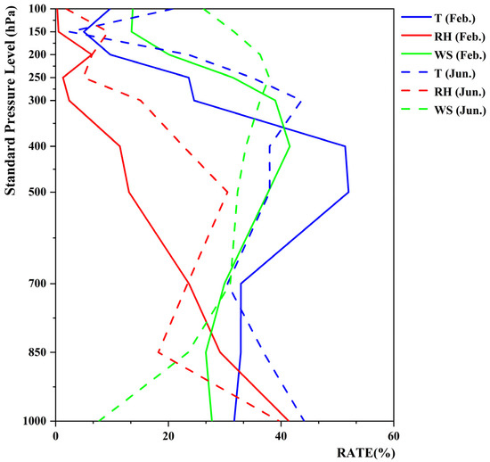
Figure 5. Improvement rate (RATE, %) for meteorological variables at different standard pressure levels (hPa) (solid lines represent February 2019; dashed lines represent June 2019; curves with the same color correspond to the same variable).

3.2. Forecast Improvement Across Underlying Surface Types

Improvements in simulation accuracy typically exhibit a heterogeneous spatial distribution, which can arise from multiple factors; among them, characteristics of the underlying surface could be one of the key factors, especially for near-surface atmospheric simulation. The underlying surface regulates boundary layer structure and development by influencing land-atmosphere exchange processes—such as heat, moisture, and momentum fluxes—and thereby affects the accuracy of numerical forecasts. To investigate how underlying surface types modulate forecast improvements by data assimilation, observation sites in this study were classified into five typical underlying surface categories: forest, grassland, cropland, urban, and water bodies. The spatial distribution of these underlying surface types is detailed in Figure 1. We then analyzed the assimilation-induced improvements for stations of each underlying surface type. Panels (a–d) of Figure 6 illustrate the RATE distributions for four near-surface meteorological variables—T₂, RH₂, and WS₁₀—across the different underlying surface types.

Figure 6. Distributions of the assimilation improvement rate (RATE, %) across different underlying surface types in February and June. (a) T₂, (b) RH₂, (c) WS₁₀.

In terms of T₂ (Figure 6a), data assimilation exhibits clear temporal and spatial heterogeneity in its impact across different underlying surface types. For nearly all underlying surface types, the RATE in summer is generally higher than in winter. This seasonal contrast was most pronounced over grassland, urban, and water body areas. In contrast, cropland shows a complex wintertime response. The data exhibit substantial dispersion, and numerous observations display negative improvement rates. This indicates that 4D-Var assimilation may produce a systematic degradation over cropland in winter. Such behavior may be related to both the special surface conditions of croplands in winter (e.g., bare soil, residue cover, and freeze–thaw cycles) and limitations in the land surface parameterization schemes under low-temperature conditions.

The relative humidity field (Figure 6b) exhibits a seasonal pattern opposite to that of the temperature field, with winter improvements generally slightly exceeding those in summer. Among these, the assimilation process demonstrates limited effectiveness in improving near-surface humidity over grassland, with median improvement rates showing negative values during both winter and summer. This indicates that the current assimilation scheme introduces a systematic negative bias when applied to near-surface humidity predictions over grassland, causing forecast results to deviate from observed values. This phenomenon may be attributed to the complexity of evapotranspiration processes occurring over grassland surfaces. Moreover, grasslands, farmlands, and urban areas all exhibit increased data dispersion during winter, with interquartile ranges markedly greater than in summer and frequent outliers. This indicates that for the same land type, the assimilation performance of humidity data across different observation sites shows greater variability in winter. This high variability likely reflects the pronounced influence of complex surface conditions during winter—such as soil freeze–thaw cycles, variations in snow cover, and vegetation dormancy—on the assimilation process of the moisture field.

Although the magnitude of improvement for wind field variables is relatively small, they nevertheless exhibit underlying surface specificity. Regarding wind speed (Figure 6c), water body areas demonstrate comparatively pronounced improvement during winter months. This phenomenon may be attributed to locally driven winds arising from wintertime thermal contrasts between water and land surfaces. As the model struggles to accurately simulate such localised circulation, its initial wind field forecasts exhibit significant bias. Consequently, incorporating observed wind data into the assimilation system corrects these forecasts, yielding markedly improved results.

The thermodynamic and dynamic characteristics of different underlying surfaces directly influence surface energy and moisture flux distributions, thereby modulating boundary layer structure and the vertical distributions of atmospheric state variables. Consequently, assimilation effectiveness varies by different underlying surface types. Water bodies consistently exhibit positive improvement rates with higher numerical values than other surfaces. This indicates a stable positive gain in forecasting through assimilation.

Conversely, grassland and cropland areas demonstrate more complex improvement patterns. Notably, grasslands exhibit systematic negative effects on humidity forecasts, while croplands show similar systematic negative effects on winter temperature forecasts. These phenomena directly point to deficiencies in current numerical model parameterisation schemes for specific land cover types.

3.3. Background Field Changes in Data Assimilation and Forecast Impact

The forecast accuracy of the NWP model is heavily dependent on the accuracy of the background field. As mentioned earlier, 4D-Var data assimilation operates by optimally combining observational information with the model background field to produce a more accurate analysis field, which is then used as the model’s background field. Figure 7 presents the spatial distribution of the monthly mean changes in the background field before and after assimilation, as well as the spatial distribution of the RATE for surface meteorological variables.

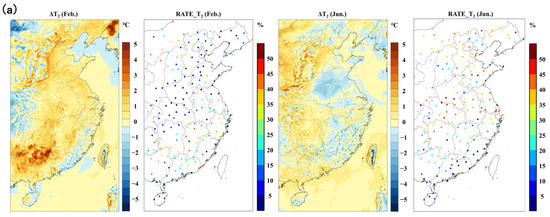
Figure 7. Spatial distributions of the monthly mean analysis increment (first and third columns) and improvement rate (RATE, %; second and fourth columns) for surface meteorological variables: (a) T₂, (b) RH₂, (c) WS₁₀ in February and June 2019.

Figure 7a presents the results for the 2 m temperature. From the February increment field, it can be observed that following 4D-Var assimilation, a regionally coherent positive increment is evident across most of the study area. The increment values are predominantly distributed between 0 °C and 2 °C, indicating that the assimilation system has implemented a correction to the background field, primarily in the form of warming, on a monthly mean basis. Comparing this with the spatial distribution of the February RATE scatter plot reveals that the temperature assimilation improvement rate is positive at most stations, with assimilation enhancing the fitting and forecasting performance of 2 m temperature to varying degrees across the vast majority of regions. The June temperature results exhibit distinct characteristics, showing an overall higher improvement rate than February and a more uniform spatial distribution. This seasonal variation reflects differences in the dominant weather systems across seasons: February’s increment field predominantly exhibits coherent warming signals, indicating background errors with large-scale, consistent characteristics—consistent with winter conditions governed by large-scale systems. Conversely, June’s increments alternate between positive and negative values, with a higher overall RATE and more uniform spatial distribution.

Figure 7b depicts the variation in 2 m relative humidity within the background field. In February, the increment field predominantly exhibits consistent negative values, indicating that assimilation has implemented a correction to the background field characterized by ‘dehumidification’ at the monthly mean level. The corresponding RATE distribution map reveals that improvements in relative humidity forecasts are primarily concentrated in the central and southern parts of the study region, with enhancement rates generally reaching 20–50%. By contrast, the June relative humidity adjustments exhibit markedly different characteristics. The intensity of negative increments has diminished, and their spatial distribution has become more complex.

Figure 7c focuses on the adjustments to the 10 m wind field and reveals the systematic correction of the near-surface dynamical field by 4D-Var. From the vector increment field, it is evident that 4D-Var imposes pronounced dynamical adjustment on the wind field. In February, the changes in wind direction point predominantly northward across much of the region, consistent with the observed prevailing wind direction in winter. In June, the wind field adjustments exhibit a more complex vector pattern, with substantial regional variations in both the direction and magnitude of the increment vectors.

The results demonstrate that 4D-Var exhibits a degree of physical consistency. The systematic warming adjustment of the winter temperature field and the cooling adjustment of relative humidity complement each other, consistent with fundamental atmospheric thermodynamic principles; the reconstruction of the wind field provides the dynamical basis for the redistribution of temperature and humidity fields. By contrast, the summer assimilation increment field exhibits greater complexity, with alternating positive and negative increments and a finer spatial distribution. This seasonal variation not only confirms that 4D-Var assimilation can accurately identify and correct the structural characteristics of background field errors across different seasons but also demonstrates the system’s robustness and precision in handling multi-scale meteorological processes.

3.4. Persistence of the Assimilation Benefits

To quantify the persistence of the positive effects of data assimilation on short-range forecasts, we stratified the daily forecasts from the CTRL and the WRFDA experiments over a continuous month by forecast lead time. Specifically, all forecasts initialized from 00 UTC were partitioned into 24 independent subsets, each corresponding to a single lead time from 1 to 24 h. For example, the 1-h subset contains the 1-h forecasts from every day within the study period, the 2-h subset contains all 2-h forecasts, and so forth. After stratification, for each forecast lead time subset, we independently computed the root mean square error (RMSE) for key near-surface variables in CTRL and WRFDA experiments, and then derived the absolute improvement in error ΔRMSE and the mean improvement rate (RATE). Meanwhile, to objectively characterize the decay of assimilation benefits with forecast lead time and assess the statistical significance of this trend, we performed linear regression analysis on the RATE series computed at each forecast lead time, using forecast lead time as the independent variable and RATE as the dependent variable. The regression coefficient directly quantifies the rate of change of RATE with time. By constructing the 95% confidence interval and prediction interval of the regression model, we evaluated the statistical uncertainty of the linear trend parameters and the expected range of variation for individual-case improvement rates, respectively. Based on the fitted intercept, slope, and their confidence bounds, we determined the forecast lead time at which the positive effects of assimilation diminish to zero, thereby objectively delineating its effective duration.

Figure 8a,b depict how the improvements in near-surface forecast due to data assimilation evolve with forecast lead time for February and June 2019, respectively. The figure indicates pronounced positive effects in both seasons: ΔRMSE remains positive throughout the 24 h following assimilation, yet the benefits exhibit a decaying trend as lead time increases. From the perspective of the physical mechanism, the early improvements likely stem from the consistent constraints on the background field imposed by 4D-Var. As the model integration progresses, systematic biases in the model and its parameterizations begin to accumulate and increasingly dominate error growth, which erodes the initial advantage—manifested as a monotonic decline of RATE with lead time.

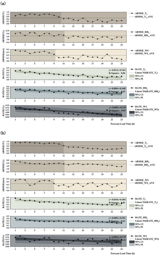
Figure 8. Evolution of assimilation benefits with forecast lead time in (a) February and (b) June 2019. In each panel, the upper three subplots display the ΔRMSE for T₂, RH₂, and WS₁₀ (the horizontal dashed line denotes the mean ΔRMSE over 23-h forecast lead times for the corresponding variable; the shaded area marks the forecast period during which ΔRMSE exceeds its mean); the lower three subplots present the corresponding improvement rate (RATE, %) and the results of the linear regression analysis, overlaid with its linear regression fit (dashed line), the 95% confidence interval (dark shading) and the 95% prediction interval (light shading).

Based on the intersection points between the ΔRMSE curves (Figure 8) and their 24-h averages, the forecast lead time can be partitioned into two phases: a strong improvement phase and a weak improvement phase. In February, T₂, RH₂, and WS₁₀ transition from the strong improvement phase to the weak improvement phase at approximately 10, 11, and 9 h, respectively; in June, the transition time occurs at about 11, 11, and 9 h, respectively. The presence of this dividing time suggests that the assimilation system provides its most pronounced improvements during roughly the first 12 h, after which its contribution gradually levels off—improvements persist, but their marginal benefit begins to diminish. Therefore, to balance forecast accuracy against computational costs, a 12-h assimilation update cycle may be an optimal choice. Notably, WS10 exhibits a relatively earlier transition time in both case months, indicating higher sensitivity than the temperature and humidity variables to the background field from assimilation.

To further clarify this decay process, we conducted linear regression analysis of RATE against forecast lead time. Using T₂ as an example, the RATE for T₂ decreased significantly with lead time in winter, with a decay rate of −0.012%/h (95% CI: −0.015–−0.010, p < 0.001), which was faster than in summer at −0.010%/h (95% CI: −0.013–−0.008, p < 0.001). This more rapid winter decay was also verified for RH₂ (winter −0.009%/h versus summer −0.005%/h) and WS₁₀ (winter −0.005%/h versus summer −0.003%/h). Despite differences in decay rates, in terms of absolute improvements, summer assimilation outperformed winter for T₂ (24-h mean ΔRMSE of 0.95 °C) and WS₁₀ (0.24 m/s), whereas winter showed a more significant improvement for RH₂ (6.73% versus 5.39%).

The faster decay rate in winter directly results in a shorter effective duration of assimilation benefits. If we extrapolate using the linear model, we can estimate the theoretical time at which assimilation benefits vanish completely, i.e., when RATE declines to 0. For T₂, the average benefit was projected to last only 30.2 h in February, markedly shorter than the 40.4 h in June. This seasonal contrast is even more pronounced for RH₂ (49.8 h vs. 70.2 h) and WS₁₀ (31.0 h vs. 45.0 h).

This phenomenon may be related to the prevailing weather regimes in different seasons: in winter, stable atmospheric stratification and weaker dynamical processes may cause model errors to grow in a more isolated and rapid manner, thereby accelerating the dissipation of information in the background field; in contrast, in summer, active convection and stronger turbulent mixing may help the coordinated information introduced by assimilation to sustain its positive influence on the model trajectory within a deeper boundary layer and over longer time scales.

Despite the decay, ΔRMSE for all variables remained consistently positive throughout the 24-h forecast window. This strongly demonstrates that the positive impact from a single 6-h assimilation cycle endures throughout an entire forecast day, and that the current cycled assimilation-forecast strategy can sustain its advantage in short-range forecasting.

3.5. Uncertainties

Uncertainties remain regarding the conclusions drawn from these data and the methods employed in this study. (1) Uncertainty in the model. Model-related uncertainties primarily stem from the idealized assumptions and seasonal applicability limits of physical parameterization schemes and surface datasets. For example, structural biases in the planetary boundary layer scheme, cumulus parameterization scheme, and microphysics schemes under different seasons and surface conditions may amplify or mask the benefits of data assimilation. Moreover, anthropogenic heat may also introduce uncertainty, as meteorological forecasts around large cities are highly sensitive to it [47]. (2) Uncertainty in assimilation window and coverage. Temporal unevenness of observations within the assimilation window and sparse multiscale spatial coverage directly affect the propagation of increments and the strength of constraints. This can lead to excessive sensitivity of the cost function at certain times and localized overfitting of the initial conditions. (3) In a two-layer nested “assimilation–forecast” workflow, cross-scale downscaling provides large-scale background constraints from the outer domain to the inner grid, but may also introduce spatiotemporal inconsistencies at the lateral boundaries, thereby affecting inner-domain forecast performance. All of these factors may contribute to uncertainty in the study’s results, but they should not diminish the significance of the present work for advancing regional numerical prediction technique optimization.

4. Conclusions

This study systematically evaluated the application effectiveness of the WRF 4D-Var data assimilation system in regional meteorological forecasting, revealing the significant role of data assimilation in enhancing the accuracy of short-term numerical weather predictions. Findings indicate that 4D-Var data assimilation delivers substantial overall improvements for both near-surface and upper-air meteorological variables. Regarding near-surface parameters, temperature, humidity, and wind fields all show enhanced forecasts post-assimilation, with temperature field improvements proving most consistent—correlation coefficients markedly increasing in both winter and summer seasons. The wind field exhibited stronger seasonal sensitivity, demonstrating a more pronounced assimilation response during summer with greater improvement than in winter. Assessments of upper-level meteorological elements revealed that assimilation improvements were primarily concentrated in the middle atmosphere between 300 and 700 hPa, indicating that 4D-Var effectively enhanced the description of atmospheric vertical structure.

Furthermore, spatial heterogeneity analysis revealed the regular distribution characteristics of the improvement effects. Significant influence of underlying surface types on assimilation performance provided crucial clues for tracing improvement causes. Water bodies exhibited optimal assimilation response compared to other land surfaces, while grassland and cropland areas revealed negative effects in specific seasons and parameters, exposing limitations of the current parameterisation scheme, requiring further refinement in subsequent studies.

Since the accuracy of numerical weather prediction fundamentally depends on the fidelity of the initial conditions, 4D-Var data assimilation achieves forecast improvement precisely by optimising these initial conditions. By comparing monthly average background field changes before and after assimilation, the study found: In February, the system applied a generalised warming correction of 0–2 °C to the 2 m temperature and a systematic ‘dehumidification’ correction to the 2 m relative humidity, while simultaneously adjusting the 10 m wind field to orient its direction more northerly. This aligns with the background error characteristics under the influence of large-scale winter weather systems. The June assimilation adjustments exhibited more complex spatio-temporal characteristics, with alternating positive and negative increments in temperature and humidity fields and finer spatial distribution, reflecting the influence of multi-scale weather processes during summer. This further confirms that 4D-Var assimilation can accurately identify and correct the structural features of background error fields across different seasons, yielding more precise results.

Finally, persistence analysis further indicates that while the positive effects of data assimilation diminish with increasing forecast lead time, they consistently maintain a beneficial contribution within the 24-h forecast window. The most significant improvements occur within the first 12 h, providing reference for subsequent studies determining optimal assimilation update frequencies. In summary, the WRF 4D-Var system demonstrates commendable performance and robustness in regional meteorological forecasting. However, its differential response across varying land surfaces (particularly grasslands and croplands) and seasonal conditions highlights key areas for future research: optimising the model’s land surface process parameterisation schemes for specific physical processes associated with particular land surfaces, and potentially integrating more targeted observational data to enhance the adaptability of the assimilation algorithm. Furthermore, based on the assimilation and forecast system developed in this study, future work should extend to longer-term simulations that include transitional seasons to construct more robust, high-precision multidimensional meteorological fields, thereby providing critical support for both regional weather forecasting and downstream air quality simulations.

References

- Bauer, P.; Thorpe, A.; Brunet, G. The Quiet Revolution of Numerical Weather Prediction. Nature 2015, 525, 47–55. [Google Scholar] [CrossRef] [PubMed]
- Gustafsson, N.; Janjić, T.; Schraff, C.; Leuenberger, D.; Weissmann, M.; Reich, H.; Brousseau, P.; Montmerle, T.; Wattrelot, E.; Bučánek, A.; et al. Survey of Data Assimilation Methods for Convective-scale Numerical Weather Prediction at Operational Centres. Q. J. R. Meteoro Soc. 2018, 144, 1218–1256. [Google Scholar] [CrossRef]
- Buehner, M.; Houtekamer, P.; Charette, C.; Mitchell, H.L.; He, B. Intercomparison of Variational Data Assimilation and the Ensemble Kalman Filter for Global Deterministic NWP. Part I: Description and Single-Observation Experiments. Mon. Weather Rev. 2010, 138, 1550–1566. [Google Scholar] [CrossRef]
- Kalnay, E. Atmospheric Modeling, Data Assimilation and Predictability; Cambridge University Press: Cambridge, UK, 2003. [Google Scholar]
- Barker, D.; Huang, X.-Y.; Liu, Z.; Auligné, T.; Zhang, X.; Rugg, S.; Ajjaji, R.; Bourgeois, A.; Bray, J.; Chen, Y.; et al. The Weather Research and Forecasting Model’s Community Variational/Ensemble Data Assimilation System: WRFDA. Bull. Amer. Meteor. Soc. 2012, 93, 831–843. [Google Scholar] [CrossRef]
- Tiwari, G.; Kumar, P. Predictive Skill Comparative Assessment of WRF 4DVar and 3DVar Data Assimilation: An Indian Ocean Tropical Cyclone Case Study. Atmos. Res. 2022, 277, 106288. [Google Scholar] [CrossRef]
- Zhang, X.; Huang, X.-Y.; Liu, J.; Poterjoy, J.; Weng, Y.; Zhang, F.; Wang, H. Development of an Efficient Regional Four-Dimensional Variational Data Assimilation System for WRF. J. Atmos. Ocean. Technol. 2014, 31, 2777–2794. [Google Scholar] [CrossRef]
- Bonavita, M.; Hólm, E.; Isaksen, L.; Fisher, M. The Evolution of the ECMWF Hybrid Data Assimilation System. Q. J. R. Meteorol. Soc. 2016, 142, 287–303. [Google Scholar] [CrossRef]
- Hersbach, H.; Bell, B.; Berrisford, P.; Hirahara, S.; Horányi, A.; Muñoz-Sabater, J.; Nicolas, J.; Peubey, C.; Radu, R.; Schepers, D.; et al. The ERA5 Global Reanalysis. Q. J. R. Meteorol. Soc. 2020, 146, 1999–2049. [Google Scholar] [CrossRef]
- Uppala, S.M.; Kållberg, P.; Simmons, A.J.; Andrae, U.; Bechtold, V.D.C.; Fiorino, M.; Gibson, J.; Haseler, J.; Hernandez, A.; Kelly, G.; et al. The ERA-40 Re-Analysis. Q. J. R. Meteorol. Soc. A J. Atmos. Sci. Appl. Meteorol. Phys. Oceanogr. 2005, 131, 2961–3012. [Google Scholar] [CrossRef]
- Dee, D.P.; Uppala, S.; Simmons, A.J.; Berrisford, P.; Poli, P.; Kobayashi, S.; Andrae, U.; Balmaseda, M.; Balsamo, G.; Bauer, P.; et al. The ERA-Interim Reanalysis: Configuration and Performance of the Data Assimilation System. Q. J. R. Meteorol. Soc. 2011, 137, 553–597. [Google Scholar] [CrossRef]
- Järvinen, H. Temporal Evolution of Innovation and Residual Statistics in the ECMWF Variational Data Assimilation Systems. Tellus A Dyn. Meteorol. Oceanogr. 2001, 53, 333–347. [Google Scholar] [CrossRef]
- Matricardi, M.; McNally, A. The Direct Assimilation of Principal Components of IASI Spectra in the ECMWF 4D-Var. Q. J. R. Meteorol. Soc. 2014, 140, 573–582. [Google Scholar] [CrossRef]
- Saha, S.; Moorthi, S.; Pan, H.-L.; Wu, X.; Wang, J.; Nadiga, S.; Tripp, P.; Kistler, R.; Woollen, J.; Behringer, D.; et al. The NCEP Climate Forecast System Reanalysis. Bull. Am. Meteorol. Soc. 2010, 91, 1015–1058. [Google Scholar] [CrossRef]
- Kalnay, E.; Kanamitsu, M.; Kistler, R.; Collins, W.; Deaven, D.; Gandin, L.; Iredell, M.; Saha, S.; White, G.; Woollen, J.; et al. The NCEP/NCAR 40-Year Reanalysis Project. In Renewable Energy; Routledge: London, UK, 2018; pp. 146–194. [Google Scholar]
- Kobayashi, S.; Ota, Y.; Harada, Y.; Ebita, A.; Moriya, M.; Onoda, H.; Onogi, K.; Kamahori, H.; Kobayashi, C.; Endo, H.; et al. The JRA-55 Reanalysis: General Specifications and Basic Characteristics. J. Meteorol. Soc. Japan. Ser. II 2015, 93, 5–48. [Google Scholar] [CrossRef]
- Onogi, K.; Tsutsui, J.; Koide, H.; Sakamoto, M.; Kobayashi, S.; Hatsushika, H.; Matsumoto, T.; Yamazaki, N.; Kamahori, H.; Takahashi, K.; et al. The JRA-25 Reanalysis. J. Meteorol. Soc. Japan. Ser. II 2007, 85, 369–432. [Google Scholar] [CrossRef]
- Huang, X.-Y.; Xiao, Q.; Barker, D.M.; Zhang, X.; Michalakes, J.; Huang, W.; Henderson, T.; Bray, J.; Chen, Y.; Ma, Z.; et al. Four-Dimensional Variational Data Assimilation for WRF: Formulation and Preliminary Results. Mon. Weather Rev. 2009, 137, 299–314. [Google Scholar] [CrossRef]
- Rabier, F. Overview of Global Data Assimilation Developments in Numerical Weather-Prediction Centres. Q. J. R. Meteorol. Soc. A J. Atmos. Sci. Appl. Meteorol. Phys. Oceanogr. 2005, 131, 3215–3233. [Google Scholar] [CrossRef]
- Lorenc, A.C.; Rawlins, F. Why Does 4D-Var Beat 3D-Var? Q. J. R. Meteorol. Soc. A J. Atmos. Sci. Appl. Meteorol. Phys. Oceanogr. 2005, 131, 3247–3257. [Google Scholar] [CrossRef]
- Rawlins, F.; Ballard, S.; Bovis, K.; Clayton, A.; Li, D.; Inverarity, G.; Lorenc, A.; Payne, T. The Met Office Global Four-Dimensional Variational Data Assimilation Scheme. Q. J. R. Meteorol. Soc. A J. Atmos. Sci. Appl. Meteorol. Phys. Oceanogr. 2007, 133, 347–362. [Google Scholar] [CrossRef]
- Vourlioti, P.; Mamouka, T.; Agrafiotis, A.; Kotsopoulos, S. Medicane Ianos: 4D-Var Data Assimilation of Surface and Satellite Observations into the Numerical Weather Prediction Model WRF. Atmosphere 2022, 13, 1683. [Google Scholar] [CrossRef]
- Xu, D.; Song, T.; Li, H.; Min, J.; Luo, J.; Shen, F. Four-Dimensional Variational Assimilation of Precipitation Data With the Large-Scale Analysis Constraint in the 21.7 Extreme Rainfall Event in China. JGR Atmos. 2025, 130, e2024JD042522. [Google Scholar] [CrossRef]
- Yang, S.; Li, D.; Duan, Y.; Chen, Y.; Liu, Z.; Huang, X.-Y. Assimilating Precipitation Data via Full-Hydrometeor Scheme in WRF 4D-Var for Convective Precipitation Forecast Associated with the Northeast China Cold Vortex (NCCV). J. Geophys. Res. Atmos. 2025, 130, e2024JD042427. [Google Scholar] [CrossRef]
- Ikuta, Y. Radar Data Assimilation in Numerical Weather Prediction Models. In Precipitation Science; Elsevier: Amsterdam, The Netherlands, 2022; pp. 743–756. [Google Scholar]
- Snyder, C.; Zhang, F. Assimilation of Simulated Doppler Radar Observations with an Ensemble Kalman Filter. Mon. Weather Rev. 2003, 131, 1663–1677. [Google Scholar] [CrossRef]
- Vendrasco, E.P.; Sun, J.; Herdies, D.L.; Frederico De Angelis, C. Constraining a 3DVAR Radar Data Assimilation System with Large-Scale Analysis to Improve Short-Range Precipitation Forecasts. J. Appl. Meteorol. Climatol. 2016, 55, 673–690. [Google Scholar] [CrossRef]
- Thépaut, J.; Courtier, P.; Belaud, G.; Lemaǐtre, G. Dynamical Structure Functions in a Four-dimensional Variational Assimilation: A Case Study. Q. J. R. Meteoro Soc. 1996, 122, 535–561. [Google Scholar] [CrossRef]
- Wang, W.; Ren, K.; Duan, B.; Zhu, J.; Li, X.; Ni, W.; Lu, J.; Yuan, T. A Four-Dimensional Variational Constrained Neural Network-Based Data Assimilation Method. J. Adv. Model. Earth Syst. 2024, 16, e2023MS003687. [Google Scholar] [CrossRef]
- Wu, Y.; Liu, Z.; Li, D. Improving Forecasts of a Record-Breaking Rainstorm in Guangzhou by Assimilating Every 10 min AHI Radiances with WRF 4DVAR. Atmos. Res. 2020, 239, 104912. [Google Scholar] [CrossRef]
- Kumar, A.; Xalxo, K.L.; Kumar, S.; Mahala, B.K.; Routray, A.; Kumar, N. Performance Assessment of 4D-VAR Microphysics Schemes in Simulating the Track and Intensity of Super Cyclonic Storm “Amphan”. Pure Appl. Geophys. 2024, 181, 3375–3391. [Google Scholar] [CrossRef]
- Lu, L.; Chen, B.; Guo, L.; Zhang, H.; Li, Y. A Regional Data Assimilation System for Estimating CO Surface Flux from Atmospheric Mixing Ratio Observations—A Case Study of Xuzhou, China. Environ. Sci. Pollut. Res. 2019, 26, 8748–8757. [Google Scholar] [CrossRef]
- Wang, Y.; Chen, Y.; Min, J. Impact of Assimilating China Precipitation Analysis Data Merging with Remote Sensing Products Using the 4DVar Method on the Prediction of Heavy Rainfall. Remote Sens. 2019, 11, 973. [Google Scholar] [CrossRef]
- Vargas, V., Jr.; Ferreira, R.C.; Pinto, O., Jr.; Herdies, D.L. Assessing the Impact of Lightning Data Assimilation in the WRF Model. Atmosphere 2024, 15, 826. [Google Scholar] [CrossRef]
- Thodsan, T.; Wu, F.; Torsri, K.; Cuestas, E.M.A.; Yang, G. Satellite Radiance Data Assimilation Using the WRF-3DVAR System for Tropical Storm Dianmu (2021) Forecasts. Atmosphere 2022, 13, 956. [Google Scholar] [CrossRef]
- Ren, J.; Huang, C.; Hou, J.; Zhang, Y.; Yang, L. Optimizing Snow Property Forecasts over the Tibetan Plateau through Hybrid Assimilation of Satellite Precipitation and Water Vapor Radiances Using WRF Model Configured with Noah-MP. J. Hydrol. Reg. Stud. 2025, 59, 102334. [Google Scholar] [CrossRef]
- National Centers for Environmental Prediction; National Weather Service; NOAA; US Department of Commerce. NCEP ADP Global Upper Air and Surface Weather Observations (PREPBUFR Format). 2008. [Google Scholar] [CrossRef]
- Copernicus Climate Change Service, Climate Data Store. ERA5 Hourly Data on Single Levels from 1940 to Present. 2023. [CrossRef]
- Copernicus Climate Change Service, Climate Data Store. ERA5 Hourly Data on Pressure Levels from 1940 to Present. 2023. [CrossRef]
- Thompson, G.; Field, P.R.; Rasmussen, R.M.; Hall, W.D. Explicit Forecasts of Winter Precipitation Using an Improved Bulk Microphysics Scheme. Part II: Implementation of a New Snow Parameterization. Mon. Weather Rev. 2008, 136, 5095–5115. [Google Scholar] [CrossRef]
- Kain, J.S. The Kain–Fritsch Convective Parameterization: An Update. J. Appl. Meteor. 2004, 43, 170–181. [Google Scholar] [CrossRef]
- Iacono, M.J.; Delamere, J.S.; Mlawer, E.J.; Shephard, M.W.; Clough, S.A.; Collins, W.D. Radiative Forcing by Long-lived Greenhouse Gases: Calculations with the AER Radiative Transfer Models. J. Geophys. Res. 2008, 113, 2008JD009944. [Google Scholar] [CrossRef]
- Hong, S.-Y.; Noh, Y.; Dudhia, J. A New Vertical Diffusion Package with an Explicit Treatment of Entrainment Processes. Mon. Weather Rev. 2006, 134, 2318–2341. [Google Scholar] [CrossRef]
- Tewari, M.; Chen, F.; Wang, W.; Dudhia, J.; LeMone, M.A.; Mitchell, K.E.; Ek, M.B.; Gayno, G.; Wegiel, J.W.; Cuenca, R. Implementation and Verification of the Unified Noah Land-Surface Model in the WRF Model [Presentation]. 2004. Available online: https://www.researchgate.net/publication/286272692_Implementation_and_verification_of_the_united_NOAH_land_surface_model_in_the_WRF_model (accessed on 25 September 2025).
- Boylan, J.W.; Russell, A.G. PM and Light Extinction Model Performance Metrics, Goals, and Criteria for Three-Dimensional Air Quality Models. Atmos. Environ. 2006, 40, 4946–4959. [Google Scholar] [CrossRef]
- Zhang, Y.; Olsen, K.M.; Wang, K. Fine Scale Modeling of Agricultural Air Quality over the Southeastern United States Using Two Air Quality Models. Part I. Application and Evaluation. Aerosol Air Qual. Res. 2013, 13, 1231–1252. [Google Scholar] [CrossRef]
- Xie, M.; Liao, J.; Wang, T.; Zhu, K.; Zhuang, B.; Han, Y.; Li, M.; Li, S. Modeling of the Anthropogenic Heat Flux and Its Effect on Regional Meteorology and Air Quality over the Yangtze River Delta Region, China. Atmos. Chem. Phys. 2016, 16, 6071–6089. [Google Scholar] [CrossRef]
Disclaimer/Publisher’s Note: The statements, opinions and data contained in all publications are solely those of the individual author(s) and contributor(s) and not of MDPI and/or the editor(s). MDPI and/or the editor(s) disclaim responsibility for any injury to people or property resulting from any ideas, methods, instructions or products referred to in the content. |
© 2025 by the authors. Licensee MDPI, Basel, Switzerland. This article is an open access article distributed under the terms and conditions of the Creative Commons Attribution (CC BY) license (https://creativecommons.org/licenses/by/4.0/).