A Loggamma Generalised Linear Model for NO₂ Emissions Data from South Africa’s Eskom’s Coal-Fired Power Stations When the Data Are Non-Normal and the Variance Is Non-Constant

Abstract

The aim of this paper is to determine if the Loggamma distribution model in a Generalised Linear Model (GLM) setup is a better model than the traditional simple linear regression model and the Lognormal-based GLM when fitted to nitrogen dioxide (NO₂) emissions data generated during the production of electricity from 13 Eskom’s coal-fuelled power stations in South Africa. The variables explaining the NO₂ emissions data are selected using backward stepwise variable selection techniques. The variables considered include the power station itself, the amount of electricity generated from the power station, the age in years of the power station, the abatement technology (filter) used at the particular power station, and the month of the year. Interaction terms between the variables are also considered. The maximum likelihood estimation (MLE) method is used to estimate parameters of the GLM, and ordinary least squares is used to estimate parameters for the regression model. The Normal, Lognormal, and Loggamma distribution models with identity link function are fitted to the NO₂ emissions data. The variance of the NO₂ emissions increases with mean emissions and the Loggamma model plots, and the explained variance metrics (the variance-function-based R² and adjusted R²) confirm the best fit to the data over the Normally distributed regression model and Lognormal-based GLM. Thus, NO₂ emissions at Eskom in South Africa can be explained and predicted by employing the Loggamma-based GLM model. The findings will assist in providing information for the development of effective strategies for mitigating air pollution and promoting sustainable practices within the energy sector in South Africa.

1. Introduction

Developing and developed countries alike are paying significant attention to the issue of atmospheric air quality and the associated climate change, as this remains one of the most critical concerns worldwide [1], and South Africa is not an exception in this endeavour. The ever-increasing levels of atmospheric air pollutants or emissions have a negative impact on human health and the overall quality of life [2,3]. Numerous epidemiological studies have demonstrated that nitrogen dioxide (NO₂) is a significant atmospheric air pollutant associated with adverse health effects in humans, including respiratory and cardiovascular diseases [4]. Nitrogen monoxide (NO) and NO₂ are the most relevant of the nitrogen oxide (NO_X) emissions to the air, causing significant pollution [5]. About 40% of NO_X emissions are produced from point sources of electric power plant boilers [6].

Air pollutants, particularly NO₂, are a major environmental concern associated with the production of electricity from coal-fuelled power stations. Eskom, the main energy producer in South Africa, uses coal as the primary source of power in electricity generation at over 13 coal-fired power stations. This method of producing electricity is responsible for the emission of dangerous pollutants, including NO₂. To safeguard human health, atmospheric air quality standards for high-priority air pollutants, including NO₂, have been imposed by authorities or regulatory bodies. This obligates Eskom to ensure and maintain adequate atmospheric air quality standards by limiting its emissions.

Air quality models are essential in all aspects of atmospheric air pollution control and planning, where prediction forms a significant component [7,8]. Mathematical models are frequently used to predict the temporal and spatial dispersion of air pollutants and to understand the effects of different atmospheric air pollutants [9]. Khare and Sharma [10] highlighted three distinct methods for modelling atmospheric air quality data, namely, deterministic modelling (analytical and numerical models), statistical modelling, and physical modelling. Sophisticated air temporal and spatial models have been employed to address the challenges associated with predicting air pollutant concentrations emitted during the production of electricity from thermal power plants, resulting in various management strategies to mitigate these harmful pollutants [11,12]. The authors of [11,12] propose a high-dimensional multi-objective optimal dispatching strategy for managing the generation of electricity with the aim of reducing emissions and emission costs [11]. The VAR-XGBoost model, based on Vector autoregression (VAR), the Kriging method, and XGBoost (Extreme Gradient Boosting), has been used to improve pollutant prediction accuracy and obtain its spatial distribution over a continuous period of time [12].

Statistical techniques involve treating the air pollution concentration as a random variable and then identifying and estimating the most suitable probability distribution to forecast the frequency of national ambient air quality standard exceedances [13,14]. The inherent properties of probability density functions make them a popular choice for modelling atmospheric emission as they cater to uncertainty in the pollutant [14].

Several statistical parent probability distributions are used to fit air pollutant concentration data. The parent statistical probability distribution fitting method involves fitting a probability distribution to emissions data, where the selected distribution serves as the “parent distribution” from which observed emissions are assumed to originate. Parent distributions concentrate their fit around where most of the data are concentrated, around the mean, mode, or median. Among these distributions are the Weibull, Gamma, Lognormal, and type V Pearson distributions [14,15].

Accurate modelling of NO₂ emissions is essential for understanding the impact of this pollutant on air quality and, hence, in developing effective mitigation strategies. Many studies involving emissions data often assume that the data have a Normal distribution and, hence, use Normally distributed regression analysis. However, this is not invariably the case, and models based on the Normal distribution are often indiscriminately applied to data that may be better handled otherwise. This is especially true of atmospheric emissions data.

The distributional assumptions made about the emission variable can have a critical impact on the conclusions drawn. An alternative approach to the Normal distribution based regression model assumption is to use some member of the family of generalised linear models.

This study investigates and compares the performance of Lognormal and Loggamma distributed Generalised Linear Models (GLMs) as potential alternatives to the traditional simple linear regression model in predicting NO₂ emissions generated during the production of electricity from Eskom’s 13 coal-fuelled power stations in South Africa. The former models are particularly good when emissions data are skewed, with an increasing variance and a heavy tail [16]. Furthermore, this study aims to identify significant variables and interactions that contribute information for the prediction of NO₂ emissions from Eskom’s coal-fuelled power stations.

The use of GLMs in environmental modelling offers several advantages over the Normal distribution based regression model. GLMs are flexible statistical models that can cater to response variables that are not even normally distributed and capture complex relationships between predictors and the response variable. By incorporating the Lognormal and Loggamma distributions, GLMs are well suited for modelling positive, right-skewed data with a variance that may increase with the mean, making them particularly relevant for NO₂ emissions data.

The rest of the paper is organised as follows: Section 2 gives the literature review, followed by the Section 3, Section 4, Section 5 and Section 6.

2. Literature Review

The literature on NO₂ emissions is very limited, especially in the South African context, but other atmospheric emissions that may be assumed to follow the same statistical distributions are discussed below.

In a study in the United Kingdom, Hadley et al. [17] investigated the distribution of annual mean daily (sulfur dioxide) SO₂ and concluded that the Lognormal distribution was a better fit for the data compared to the Normal distribution. In another study on the distribution of particulate matter emissions in Washington, Rumburg et al. [18] concluded that the three-parameter Lognormal distribution and a generalised extreme value distribution (GEVD) had the best fit to the data. Kao and Friedlander [19] further observed that the frequency distribution of (non-reactive) aerosol components of particulate matter PM₁₀ (particulate matter of size 10 micrometres or less) and the source contributions, for most sources, followed an approximately Lognormal distribution in the South Coast Air Basin (SoCAB), United States of America.

Three theoretical distributions (Lognormal, Weibull, and type V Pearson) were used to fit PM₁₀ concentrations in the Belgrade urban area for the 2003–2005 period. The type V Pearson distribution was found to be the most appropriate in representing PM₁₀ daily average concentrations [20]. In a similar study by Lu, the Gamma distribution was the best of the three theoretical parent frequency distributions (Lognormal, Weibull, and Gamma) in representing the distribution of high PM₁₀ concentrations in central Taiwan [15]. The measured data on NO₂, PM₁₀, PM_2.5, and SO₂ in Santiago were fitted using the type V Pearson distribution [21]. In their study, Zhang et al. [22] investigated the statistical distribution of automobile emissions, namely, carbon monoxide (CO) and hydrocarbons (HCs), from various locations in the United States. The automobile emissions followed a statistically Gamma-distributed pattern.

Other techniques to model emission data have been used in the past. Sahsuvaroglu et al. [23] used a land use regression (LUR) model to predict NO₂ concentrations in Hamilton, Ontario, Canada. In other studies, such as those by Boznar et al. [24], Gardner and Dorling [25], Comrie [26], among others, a component of machine learning, namely, the multilayer neural network technique, was used to forecast emissions data.

Atmospheric emission data are rarely modelled using GLMs, and yet, data are not always Normally distributed. The current study uses Lognormal and Loggamma distributed based GLMs to fit the NO₂ emissions data from Eskom’s 13 coal-fuelled power stations and compare them with a Normal distribution based regression analysis in this paper.

3. Methodology

This section discusses linear regression and the GLM models. In regression analysis, the data are assumed to be Normally distributed.

3.1. Linear Regression

The following model will be fitted stepwise to the NO₂ emissions data initially. Analysis of Covariance (ANCOVA) will be used since the response variable is continuous and the explanatory variables are both continuous and categorical. The stepwise procedure implies that only the significant variables may be used in the final model. Backward stepwise variable selection is used to try and find the best model. This model selection procedure allows one to start with a more complex model that includes all possible or available variables and the interaction terms of these variable terms.

The full model in this case is given as:

$$\begin{array}{c}{Y}_{pqts}\equiv {\beta }_0+{{\beta }_{1}x}_{pqts}+{\beta }_2{Age}_t+{\gamma }_p+{\alpha }_q+{\tau }_s+{\alpha }_q{\tau }_s+{\gamma }_p{\alpha }_q+x_{pqts}{Age}_t+x_{pqts}{\gamma }_p+x_{pqts}{\alpha }_q+x_{pqts}{\tau }_s\hfill \\ \hspace{1em}\hspace{1em}\hspace{1em}\hspace{1em}\hspace{1em}\hspace{1em}+{Age}_t{\alpha }_q+{Age}_t{\tau }_s+{Age}_t{\gamma }_p+x_{pqts}{\gamma }_p{\tau }_s+x_{pqts}{\gamma }_p{\alpha }_q+x_{pqts}{Age}_t{\gamma }_p+x_{pqts}{Age}_t{\alpha }_q\hfill \\ \hspace{1em}\hspace{1em}\hspace{1em}\hspace{1em}\hspace{1em}\hspace{1em}+x_{pqts}{Age}_t{\tau }_s+{Age}_t{\gamma }_p{\alpha }_q+{Age}_t{\gamma }_p{\tau }_s+{Age}_t{\alpha }_q{\tau }_s+x_{pqts}{\gamma }_p{\alpha }_q{\tau }_s+{\gamma }_p{Age}_t{\alpha }_q{\tau }_s\hfill \\ \hspace{1em}\hspace{1em}\hspace{1em}\hspace{1em}\hspace{1em}\hspace{1em}+x_{pqts}{Age}_t{\gamma }_p{\alpha }_q+x_{pqts}{Age}_t{\gamma }_p{\tau }_s+x_{pqts}{Age}_t{\alpha }_q{\tau }_s+x_{pqts}{Age}_t{\gamma }_p{\alpha }_q{\tau }_s+{\epsilon }_{pqts},\hfill \end{array}$$

(1)

where

“$Y_{pqts}$” is the response, i.e., NO₂ emission in tons from filter $q$ in plant $p$ at time $t$ in month $s$.

$x_{pqts}{Age}_t{\gamma }_p{\alpha }_q{\tau }_s$ is the joint effect on NO₂ emission of electricity sent out in Gigawatt-hours (by filter $q$ in plant $p$ at given age, at time $t$ in month $s$), ${Age}_t$of the power plant at time t (in years), the $p^{th}$ plant, $q^{th}$ filter and the $s^{th}$ month.

$x_{tpqs}{Age}_t{\gamma }_p{\tau }_s$ is the joint effect of electricity sent out in Gigawatt-hours (by filter $q$ in plant $p$ at a given age at time $t$ in month s), ${Age}_t$ of the power plant at time t (in years), the $p^{th}$ plant and the $s^{th}$ month. It means the difference in effect of electricity sent out in Gigawatt-hours (by filter $q$ in plant $p$ at given age at $t$ in month $s$) on NO₂ emission in tons depending on the ${Age}_t$of the power plant at time t (in years), the $p^{th}$ plant and the $s^{th}$ month.

${\epsilon }_{pqts}~N(0,{ \sigma }^2)$ is the error term.

Similar interpretations can be made for the other interaction parameters. The model includes all the variables recorded in this study, including interaction terms between the variables.

3.1.1. Model Selection

Backward Model Selection Procedure

The backward stepwise variable selection method eliminates each explanatory variable that is not statistically significant at each step. Schwarz’s Bayesian Information Criterion (BIC), the Akaike Information Criteria (AIC), the residuals, and other plots are used to check if the elimination of an explanatory variable simplifies to a good and adequate model or not; hence, they are also used to determine the best-fitting model. The lowest values of BIC and AIC are associated with the best model. The BIC and AIC formulae are given as follows [27].

$$BIC=-2l\left(\widehat{\theta };y\right)+2p\times \mathrm{l}\mathrm{n}(\mathrm{n})$$

(2)

and

$$AIC=-2l\left(\widehat{\theta };y\right)+2p,$$

(3)

where $l\left(\widehat{\theta };y\right)$ is the log-likelihood, $p$ is the number of parameters, and $n$ is the number of observations.

The best variable fitting model is found for the Normal, Lognormal, and Loggamma distribution models, all with identity link functions. The elimination process starts with a model containing all the following explanatory variables: power station, electricity sent out in Gigawatt-hours from the power station, age in years of the power station, type of filter used at the power station, month of emission, and all their interaction terms.

Box plots, histograms, the Kolmogorov–Smirnov test, and quantile–quantile (QQ) plots are used to check the Normality assumption of the data and residuals. A symmetric and bell-shaped histogram suggests the data follow a Normal distribution and the model residuals suggest a good fit.

The best model is to be selected between the Normal, Lognormal, and the Loggamma distribution based GLMs, as discussed later.

3.2. Generalised Linear Models

The data used in a classical regression model are assumed to be symmetric and to belong to a Normal distribution with a constant variance, ${\sigma }^2$. However, in practice, it is common to find data in the form of continuous measurements, where Normality, symmetry, and homoscedasticity assumptions do not hold. In such cases, the Lognormal and Loggamma distributions may be better candidates to model the data, especially if the variance of the data is suspected to increase with the mean of the data, that is, for some constant ${\sigma }^2$, if the variance of the data is of the form:

$$Var\left(Y\right)={\sigma }^2{\left[E\right(Y\left)\right]}^2={\sigma }^2{\mu }^2.$$

(4)

3.2.1. The Logarithmic Transformation

Generally, transforming the data has three main purposes: stabilising the variance in the response variable (homoscedasticity), improving the model fit to the data (additive effects), and making the distribution of the response variable closer to the Normal distribution (thus, approximating symmetry) [28].

For a random variable $Y$ with a variance that is proportional to the mean, as in Equation (4), one of the variance-stabilising transformations involves taking the logarithm of the response, $\ln Y$, such that:

$Var\left(\ln Y\right)\approx {\left[{\displaystyle \frac{\partial \ln Y}{\partial y}}{|}_{y=\mu }\right]}^{2}Var\left(Y\right)={\displaystyle \frac{1}{{\mu }^2}}{\sigma }^2{\mu }^2={\sigma }^2$ is a constant [29].

This transformation also has a normalising effect on a distribution that is positively skewed [30].

3.2.2. The Lognormal Distribution

Suppose the random variable $X$ follows a Normal distribution with parameters $\mu$ and ${\sigma }^2$. Consider the transformation $X=\ln Y$ or, equivalently, $Y=e^X$; then, $Y~Lognormal\left(\mu ,{\sigma }^2\right)⟺\ln Y~Normal(\mu ,{\sigma }^2)$. That is to say, the logarithm of a random variable follows a Normal distribution. Therefore, a random variable $Y$ with positive continuous values follows a Lognormal distribution if it has a probability density function that can be written in the following form [16]:

$$f\left(y;\mu ,{\sigma }^2\right)={\displaystyle \frac{1}{\sqrt{2\pi {\sigma }^2}}}\exp \left[-{\displaystyle \frac{{\left(\ln y-\mu \right)}^2}{2{\sigma }^2}}\right]\left({\displaystyle \frac{1}{y}}\right),-\infty \le \mu \le \infty ,y>0,\sigma >0,$$

(5)

where ${\displaystyle \frac{1}{y}}$ is the Jacobian of the transformation $x=\ln y$.

The distribution has:

$$E\left\{y\right\}={\mu }_Y=\mathrm{e}\mathrm{x}\mathrm{p}(\mu +{\displaystyle \frac{{\sigma }^2}{2}})\mathrm{and} {\sigma }_Y^2=Var\left(y\right)=\mathrm{e}\mathrm{x}\mathrm{p}{(\mu +\sigma )}^2\left[\exp \left({\sigma }^2\right)-1\right].$$

The Lognormal distribution has a constant coefficient of variation, as shown below

$$CV\left(Y\right)={\displaystyle \frac{\sqrt{Var\left(y\right)}}{E\left(Y\right)}}$$

$$CV\left(Y\right)={\displaystyle \frac{\sqrt{u^2{\theta }^2}}{u}}$$

$$CV\left(Y\right)={\displaystyle \frac{u\theta }{u}}=\theta =\sqrt{(\exp \left({\sigma }^2\right)-1)}$$

where $\theta =\sqrt{(\exp \left({\sigma }^2\right)-1)}$, ${\mu }_Y=\exp \left(\mu +{\displaystyle \frac{{\sigma }^2}{2}}\right),$ and $Var\left(y\right)=\mathrm{e}\mathrm{x}\mathrm{p}{(\mu +\sigma )}^2\left[\exp \left({\sigma }^2\right)-1\right].$

The variance of the Lognormal model increases with the mean. It increases with the mean such that the coefficient of variation is constant. Lognormal modelling can be used to compensate for such increases with the mean such that the residual distribution results in homoscedasticity.

3.2.3. The Loggamma Distribution

Let $X$ be a random variable that has a Gamma distribution if it has a probability density function that can be written in the form

$$f\left(y;\mu \right)={\displaystyle \frac{1}{\mathsf{\Gamma }\left(v\right)\mathrm{y}}}{\left({\displaystyle \frac{vy}{\mu }}\right)}^{v}exp\left(-vy/\mu \right) , v={\displaystyle \frac{1}{{\sigma }^2}}>0, \mu , y>0$$

(6)

with the mean and variance given by:

$E\left\{y\right\}=\mu$ and $Var\left(y\right)={\displaystyle \frac{{\mu }^2}{v}}$, respectively, such that the coefficient of variation of $y$ is:

$$CV\left(y\right)={\displaystyle \frac{\sqrt{Var\left(y\right)}}{E\left(y\right)}}={\displaystyle \frac{\sqrt{\frac{{\mu }^2}{v}}}{\mu }}=\sqrt{{\displaystyle \frac{1}{v}}}={\displaystyle \frac{1}{\sqrt{v}}}={\displaystyle \frac{1}{\sqrt{\frac{1}{{\sigma }^2}}}}=\sigma ,$$

(7)

since $v={\displaystyle \frac{1}{{\sigma }^2}}$.

Unlike the Normal distribution with the constant variance assumption, the Gamma model has a variance that increases with the mean. The variance increases with the mean in such a way that the coefficient of variation is again a constant. The Gamma model can be used to compensate for such increases in variance with the mean in modelling.

Considering the transformation $X=\ln Y$ or, equivalently, $Y=e^X$; then, $Y~Loggamma\left(\alpha ,\lambda \right)⟺\ln Y~Gamma(\alpha ,\lambda )$.

That is, the logarithm of a random variable follows a Gamma distribution. Taking the logarithmic transform of the data will further tame the variance of the data. Therefore, a random variable $Y$ with positive continuous values follows a Loggamma distribution if it has a probability density function that can be written in the following form [16]:

$$f\left(y;\mu \right)={\displaystyle \frac{1}{\mathsf{\Gamma }\left(\alpha \right)\mathrm{y}}}{\left(\ln y\right)}^{\alpha -1}exp\left(-\lambda \ln y\right)={\displaystyle \frac{{\left(\ln y\right)}^{\alpha -1}}{\mathsf{\Gamma }\left(\alpha \right)y^{\lambda +1}}}, 1<y<\infty ,$$

(8)

with mean and variance given by:

$E\left\{y\right\}={\mu }_Y={\displaystyle \frac{{\lambda }^{\alpha }}{{(\lambda -1)}^{\alpha }}}$, for $\lambda >1,$ and ${\sigma }_Y^2=Var\left(y\right)={\displaystyle \frac{{\lambda }^{\alpha }}{{(\lambda -2)}^{\alpha }}}-{\displaystyle \frac{{\lambda }^{2\alpha }}{{(\lambda -1)}^{2\alpha }}}$, for $\lambda >2,$ respectively.

The tail of the distribution is given by $\overline{F}(x)~{\displaystyle \frac{{\lambda }^{\alpha -1}{\left(\ln y\right)}^{\alpha -1}}{\mathsf{\Gamma }\left(\alpha \right)y^{\lambda }}}$ [31].

The Normal distribution assumes the data are symmetric. However, emission data are not always symmetric and may be skewed. In such cases, the Loggamma distribution provides a good alternative. This distribution can also cater to heavy-tailed data [32] since it belongs to Pareto-type tail distributions; see Albrecher et al. [32] for details.

Broadly speaking, under the Loggamma distribution, a unimodal distribution represents mid-sized data, and large observations are represented by a Pareto-like tail [33].

3.2.4. The Exponential Family Distribution

Let $Y$ be a random variable with a distribution in the exponential family and a pdf $f\left(y;\mu \right)$ in the standard form:

$$f\left(y;\mu \right)=\exp \left[a\left(y\right)b\left(\mu \right)+c\left(\mu \right)+d\left(y\right)\right]$$

(9)

The distribution is said to be in canonical form when $a\left(Y\right)=y$.

In order to be a GLM, a model must have the three components, namely, an error distribution, a linear predictor, and a link function [27]. The Lognormal and Loggamma distributions are in the exponential family of distributions for the following reasons:

1.

Error Distribution.

The Lognormal distribution has independent response variables $Y_{1,}{Y}_2,\dots ,Y_n$ with the pdf given in Equation (5) and rewritten as

$$f\left(y;\mu \right)=\mathrm{e}\mathrm{x}\mathrm{p}\left\{\mathrm{l}\mathrm{n}(y).{\displaystyle \frac{\mu }{{\sigma }^2}}-{\displaystyle \frac{{\mu }^2}{2{\sigma }^2}}-\left[{\displaystyle \frac{{\mathrm{l}\mathrm{n}\left(y\right)}^2}{2{\sigma }^2}}+{\displaystyle \frac{1}{2}}\mathrm{l}\mathrm{n}(2\pi {\sigma }^2{y}^2)\right]\right\},$$

(10)

where $a\left(y\right)=\mathrm{l}\mathrm{n}\left(y\right)$, $b\left(\mu \right)={\displaystyle \frac{\mu }{{\sigma }^2}}$, $c\left(\mu \right)=-{\displaystyle \frac{{\mu }^2}{2{\sigma }^2}}$, and $d\left(y\right)=-{\displaystyle \frac{{\ln \left(y\right)}^2}{2{\sigma }^2}}-{\displaystyle \frac{1}{2}}\ln \left(2\pi {\sigma }^2{y}^2\right).$

The Loggamma distribution assumes independent response variables $Y_{1,}{Y}_2,\dots ,Y_n$ with the pdf given in Equation (8) and rewritten as

$$f\left(y; \lambda \right)=\exp \left\{-\lambda \ln y+\alpha \ln \lambda +[\left(\alpha -1\right)\ln \left(\ln y\right)-\ln y-\ln \mathsf{\Gamma }\left(\alpha \right)]\right\}$$

(11)

where $a\left(y\right)=\ln y,b\left(\lambda \right)=-\lambda$ is the natural parameter of the distribution, $c\left(\lambda \right)=\alpha \ln \lambda ,$ and $d\left(y\right)=\left(\alpha -1\right)\ln \left(\ln y\right)-\ln y-\ln \mathsf{\Gamma }\left(\alpha \right)$.

2.

Linear Predictor.

The linear predictor ${\eta }_{tpqs}$ is chosen when, for instance, the parameters $\beta$ and explanatory variable vector $X_i$ are such that

$${\eta }_{tpqs}\equiv {\beta }_0+{\beta }_1{x}_{tpqs}+{\beta }_2{Age}_t+{\gamma }_p+{\alpha }_q+{\tau }_s$$

(12)

where $X_i=\left[1,x_{i1},x_{i2}\dots ,x_{ip}\right]=[1,x_{tpqs},{Age}_t\dots ,December]$.

3.

Link Function.

There exists a monotone link function $g$ such that $g\left({\mu }_i\right)={\eta }_i={x^{’}}_i\beta ,i=1,\dots ,n$.

Box and Cox [34] introduced a flexible family of transformations: the power transformations. For a given parameter $\lambda$, the transformation is defined by

$$g\left(y\right)=\left(\begin{array}{cc}{\displaystyle \frac{y^{\lambda }-1}{\lambda }},& for \lambda \ne 0\\ \log \left(y\right),& for \lambda =0.\end{array}\right.,$$

(13)

To determine the most suitable data transformation, the Box–Cox method is used to estimate the $\lambda$ value.

Generally, transformations are used for three purposes: stabilising the response variance, making the distribution of the response variable closer to a normal distribution, and improving the fit of the model to the data. The last objective could include model simplification, say, by finding a suitable link function. Sometimes, a transformation will be reasonably effective in simultaneously accomplishing more than one of these objectives.

According to Myers et al. [28], the natural values for $\lambda$ are as follows:

• When $\lambda =0,$ then log transform the data.

• When $\lambda =1,$ then there is no need to transform the data (identity link function).

• When $\lambda ={\displaystyle \frac{1}{2}},$ then square root transform the data.

• When $\lambda =-1,$ then inverse transform the data.

In the case of the dataset used in this study, $\lambda$ is approximated to 1 ($\lambda \cong 1$). Although the confidence interval [0.6, 0.7] in the Box–Cox plot in Figure 1 does not contain a 1, the result is deemed close enough to warrant no transformation of the data. This value of $\lambda \cong 1$ is obtained by rounding off [35] since the confidence interval does not also contain a 0.5. For practical reasons, it makes sense to assume ($\lambda \cong 1$). Therefore, there is no need to transform the data further, especially in the linear regression case.

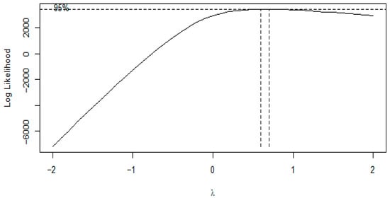
Figure 1. The Box–Cox plot for nitrogen dioxide (NO₂) emissions data.

There exists a monotone link function $g,$ such that $g\left({\mu }_i\right)={\eta }_i={x^{’}}_i\beta ,i=1,\dots ,n$, for the NO₂ emissions data. An appropriate link function is chosen based on the nature of the data of interest. With the response variable being continuous and positive, the link function may be chosen from the following examples,

$$\mathrm{Identity}: g\left({\mu }_{pqt}\right)={\mu }_{pqt}={\beta }_0+{\beta }_1{x}_{pqt}+{\beta }_2{Age}_t+{\gamma }_p+{\alpha }_q+{\tau }_s,$$

(14)

$$log : g\left({\mu }_{pqt}\right)={\mathrm{l}\mathrm{o}\mathrm{g}(\mu }_{pqt})={\beta }_0+{\beta }_1{x}_{pqt}+{\beta }_2{Age}_t+{\gamma }_p+{\alpha }_q+{\tau }_s$$

(15)

Linear regression is a GLM with an identity link and Normally distributed data. In a generalised linear model, the mean may be transformed by the link function instead of transforming the emission itself.

The two methods of transformation can lead to quite different results; for example, the mean of log-transformed emissions is not the same as the logarithm of the mean emissions. In general, the former cannot easily be transformed into a mean emission. Transforming the mean often allows the results to be more easily interpreted, especially because the mean parameters remain on the same scale as the measured emissions. Since the Loggamma GLM is compared to the linear regression and Lognormal GLM, the identity link function is used for all three models.

3.2.5. Model Selection

Similar to the linear regression model above, forward selection, Schwarz’s Bayesian Information Criterion (BIC), residual plots, and residuals against predicted value plots are used to select variables with a significant effect in the prediction of NO₂ emissions. Backward selection is considered in determining the best-fitting model with interaction variable terms.

For all GLMs, the MLE method is the main method of estimation used [36]. In the MLE method, a standard assessment involves comparing the fitted model with a fully or saturated specified model [37]. Suppose ${\beta }_{max}$ is the parameter vector of the saturated model and $b_{max}$ is the ML estimator of ${\beta }_{max}$. $L(b_{max};y)$ denotes the likelihood function of the saturated model evaluated at $b_{max}$. For the maximum value $L(b;y)$ of the likelihood function of the model of interest, we have $l(b_{max};y)$ and $l(b;y)$ as the associated log-likelihoods [27], such that the deviance $\left(D\right)$ is given by

$$D=2\log \left(\lambda \right)=2\left[l\left(b_{max};y\right)-l(b;y)\right].$$

(16)

The deviance against the degrees of freedom is used to determine if a distribution model is a good fit to the data or not. A model with a deviance that is smaller than the degrees of freedom is considered a good fit.

4. Results

This section gives the results for all the 13 power stations that will be used in modelling NO₂ emissions (in tons per month). The data are monthly NO₂ emissions per Eskom station, for a maximum period of 108 months (between 2005 and 2014). These data are presented in the Supplementary Materials and include the variables, NO₂ emissions, power station itself, the amount of electricity generated from the power station, the age in years of the power station, the abatement technology (filter) used at the particular power station, and the month of the year. Table 1 gives information on the power stations, including the installed/nominal capacity of the power station and the location [38].

Table 1. Eskom coal-fired stations, their installed capacities, and their locations.

Power Station	Installed/Nominal Capacity in Mega Watts (MW).	Location
Arnot	2352 (1 × 370, 1 × 390, 2 × 396, 2 × 400)	Middelburg, Mpumalanga
Camden	1510 (2 × 200, 1 × 195, 2 × 190, 1 × 170, 1 × 180, 1 × 185)	Ermelo, Mpumalanga
Duvha	3600 (6 × 600)	Witbank, Mpumalanga
Grootvlei	1200 (6 × 200)	Balfour, Mpumalanga
Hendrina	1965 (8 × 200, 1 × 195, 1 × 170)	Hendrina, Mpumalanga
Kendal	4116 (6 × 686)	Witbank, Mpumalanga
Komati	940 (5 × 100, 2 × 125, 2 × 95)	Middelburg, Mpumalanga
Kriel	3000 (6 × 500)	Kriel, Mpumalanga
Lethabo	3708 (6 × 618)	Sasolburg, Free State
Majuba	4110 (3 × 657, 3 × 713)	Volksrust, Mpumalanga
Matimba	3990 (6 × 665)	Lephalale, Limpopo
Matla	3600 (6 × 600)	Kriel, Mpumalanga
Tutuka	3654 (6 × 609)	Standerton, Mpumalanga

Note: Adapted from “Eskom-partnering for a sustainable future, Integrated Report 2011” (https://www.eskom.co.za/wp-content/uploads/2021/10/eskom-ar2011.pdf, accessed on 29 July 2025). Copyright 2011, by Eskom.

The analysis was performed using the SAS Studio application under SAS OnDemand for Academics (SAS 9.4 M8, SAS Institute, Cary, NC, USA).

4.1. Descriptive Statistics

In Table 2, in the given period, the highest amount of monthly NO₂ emissions was 13 923.25 tons, which occurred in March 2009 at the Majuba (in Volksrust, Mpumalanga province, South Africa) power station when it was 13.25 years old. On the other hand, the lowest amount of monthly NO₂ emissions of 26.42 tons was recorded in September 2009 at the Komati (in Middelburg, Mpumalanga province) power station.

Table 2. Summary statistics for NO₂ emissions, electricity sent out, and relative NO₂ emissions per power station, ordered according to efficiency of a power station based on the relative efficiency, from most efficient (rank = 1) to least efficient (rank = 13).

Power Station	N	Variable	Min	Mean	Median	Std Dev	Max
MATIMBA	108	NO2 Emissions (tons)	4142.00	5558.08	5624.94	521.94	6857.59
Rank = 1		Electricity Sent Out (GWhs)	1727.27	2299.79	2348.27	207.28	2638.78
		Relative NO2 Emissions (tons/GWhs)	2.18	2.42	2.40	0.09	3.04
KENDAL	108	NO2 Emissions (tons)	5385.00	8287.38	8141.92	1398.43	11,266.00
Rank = 2		Electricity Sent Out (GWhs)	1621.82	2165.12	2219.15	229.91	2561.66
		Relative NO2 Emissions (tons/GWhs)	2.90	3.84	3.75	0.58	6.08
ARNOT	108	NO2 Emissions (tons)	2309.00	3963.02	4014.50	574.44	5063.00
Rank = 3		Electricity Sent Out (GWhs)	635.10	1007.98	997.95	138.46	1250.90
		Relative NO2 Emissions (tons/GWhs)	3.39	3.94	3.87	0.36	5.75
HENDRINA	108	NO2 Emissions (tons)	2665.00	4097.93	4195.95	578.74	5723.00
Rank = 4		Electricity Sent Out (GWhs)	586.47	977.44	991.17	152.13	1254.61
		Relative NO2 Emissions (tons/GWhs)	2.94	4.22	4.22	0.33	5.94
DUVHA	108	NO2 Emissions (tons)	4671.00	7532.95	7674.96	1233.31	10,234.00
Rank = 5		Electricity Sent Out (GWhs)	1103.93	1770.21	1808.75	306.15	2323.06
		Relative NO2 Emissions (tons/GWhs)	3.83	4.27	4.25	0.19	4.81
GROOTVLEI	60	NO2 Emissions (tons)	316.22	1800.71	1861.07	723.86	3203.00
Rank = 6		Electricity Sent Out (GWhs)	138.85	418.92	441.66	160.80	679.52
		Relative NO2 Emissions (tons/GWhs)	1.52	4.30	4.25	0.56	5.72
CAMDEN	96	NO2 Emissions (tons)	52.00	2623.43	2702.75	1001.63	4380.00
Rank = 7		Electricity Sent Out (GWhs)	11.66	558.34	601.31	174.97	815.05
		Relative NO2 Emissions (tons/GWhs)	1.89	4.62	4.68	0.68	5.84
TUTUKA	108	NO2 Emissions (tons)	4424.00	7664.55	7647.72	1507.84	10,696.00
Rank = 8		Electricity Sent Out (GWhs)	1055.83	1612.46	1622.52	242.69	2125.02
		Relative NO2 Emissions (tons/GWhs)	3.28	4.76	5.00	0.70	6.04
LETHABO	108	NO2 Emissions (tons)	6696.00	9755.43	9640.00	1352.38	13,059.00
Rank = 9		Electricity Sent Out (GWhs)	1256.34	2043.16	2056.89	228.73	2524.13
		Relative NO2 Emissions (tons/GWhs)	4.17	4.78	4.66	0.39	5.60
MATLA	108	NO2 Emissions (tons)	6495.00	9428.22	9591.00	1114.03	11,512.92
Rank = 10		Electricity Sent Out (GWhs)	1282.41	1849.64	1851.63	245.12	2396.69
		Relative NO2 Emissions (tons/GWhs)	4.15	5.12	5.16	0.36	6.39
MAJUBA	108	NO2 Emissions (tons)	5400.00	10,433.49	10,494.68	1815.99	13,923.25
Rank = 11		Electricity Sent Out (GWhs)	1003.58	1878.74	1902.14	302.23	2461.67
		Relative NO2 Emissions (tons/GWhs)	4.88	5.55	5.55	0.31	7.36
KOMATI	60	NO2 Emissions (tons)	26.42	1422.23	1162.44	772.09	2788.00
Rank = 12		Electricity Sent Out (GWhs)	4.85	243.96	206.24	133.28	492.24
		Relative NO2 Emissions (tons/GWhs)	4.43	5.86	5.84	0.58	8.63
KRIEL	108	NO2 Emissions (tons)	4404.00	8466.14	8584.82	1506.90	12,634.64
Rank = 13		Electricity Sent Out (GWhs)	761.18	1427.53	1448.45	267.28	1863.96
		Relative NO2 Emissions (tons/GWhs)	4.18	5.97	5.91	0.54	7.63

Komati power station emitted the lowest average monthly NO₂ of 1422.23 tons, while Majuba power station emitted the highest at 10,433.49 tons per month.

The average monthly electricity sent out, measured in GWhs, was highest at Matimba power station (located in Lephalale, in the Limpopo province, South Africa), while Komati power station had the lowest average monthly electricity sent out.

In 2014, the age of the oldest power station was 44 years, while the youngest was 18 years, with Hendrina (in Mpumalanga province) being the former and Majuba (Volksrust, Mpumalanga) being the latter.

The efficiency of a power station is measured by calculating the relative NO₂ (tons/Gigawatt-hours) rather than just observing the amount of NO₂ emissions (in tons), calculated as follows:

$$relative emission \left(r.e\right)={\displaystyle \frac{{NO}_2 emission (in tons)}{Electricity sent out (in Gigawatts hours)}}.$$

(17)

Matimba power station was determined to be the most efficient out of the 13 power stations; hence, it received a rank of 1, based on its lowest average relative NO₂ emissions (tons/GWhs); see Table 2. This indicates that Matimba produces the highest amount of electricity per emission. Kriel (in Mpumalanga province) power station was found to be the least efficient, with a rank of 13, and Komati power station had a rank of 12; see Table 2.

In Figure 2, the joint fabric filter and electrostatic precipitators, along with flue gas conditions, are abatement technologies identified as being associated with the highest efficiency with lowest values of average relative emissions. The electrostatic precipitators are associated with the lowest efficiency with the highest relative emissions.

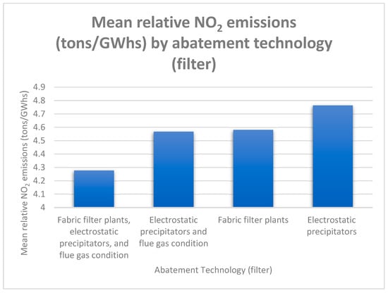
Figure 2. Mean relative NO₂ emissions (tons/GWhs).

Eskom has some power stations, namely, Grootvlei, Camden, and Komati, that stopped functioning and became mothballed from non-usage in the late 1980s and 1990s due to excess capacity. These plants were later returned to service in response to high demand for electricity, which Eskom could not meet without load shedding, and to reduce the demand pressure experienced in the already operating power stations. The units in Grootvlei were recommissioned between 2008 and 2011, those in Camden between 2005 and 2008, and those in Komati between 2009 and 2013 [39,40].

4.2. Tests for Autocorrelation and Collinearity

The Durbin–Watson (DW) test statistic and ACF and PACF plots were used to test the presence of autocorrelation in the data.

The DW test was conducted to test the presence of correlation between two successive observations in the data. The computed DW statistic is 1.325. This indicates the presence of autocorrelation in the data. However, no autocorrelation after log transforming the response was found since the DW statistic of 1.513 is between 1.5 and 2.5 [41,42,43,44,45,46].

The ACF and PACF results are presented in Figure 3 and Figure 4.

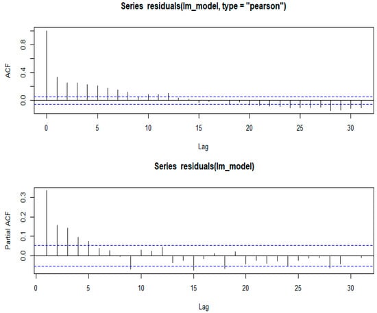
Figure 3. ACF and PACF for NO₂ emissions from 13 of Eskom’s coal-fired power stations.

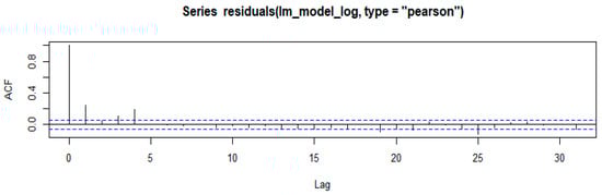
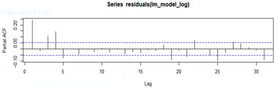
Figure 4. ACF and PACF for log (NO₂ emissions) from 13 of Eskom’s coal-fired power stations.

The first results presented in Figure 3 show the AFC and PACF of the linear regression model given in Equation (18), below, fitted before log transformation of the response, i.e., NO₂ emissions. The ACF and PACF results for the log-transformed NO₂ emissions are given in Figure 4.

Checking for collinearity among paired continuous explanatory variables is crucial prior to fitting a regression model and other models. The presence of such a relationship implies that knowing one variable allows us to predict the other, resulting in both variables attempting to explain the same variability in the response variable.

To detect collinearity, the variance inflation factors ${VIF}_i={\displaystyle \frac{1}{1-R^2}},i=1,\dots .,n,$ of the explanatory variables are used. If ${VIF}_i>10$, it is a cause for concern [47].

For instance, considering age (in years) and electricity sent out (in GWhs), ${VIF}_i=1.71897<10$. This suggests that the two explanatory variables are not significantly dependent on each other.

4.3. Model Selection

Since there is no collinearity, one can proceed to select a model that includes only the significant explanatory variables in predicting NO₂ emissions (in tons). To determine this, the BIC and AIC are used. Other variables are eliminated at each step from the model in Equation (1) using backward selection.

Backward Selection

The BIC and AIC values are used to determine if a term should be included in the final model or not. The model with the lowest BIC and AIC values is considered the best model.

In all three models, namely, the linear regression model assuming Normality of data, the Lognormal distribution model, and the Loggamma distribution model, the final model includes the interaction terms electricity × station and age × station and the explanatory variables electricity sent out (in GWhs), age of the power station (in years), and power station used. All other explanatory variables (i.e., abatement technology and month of emission) and interaction terms from the model in Equation (1) are excluded in the backward selection elimination process. This is performed so that the final model only consists of the significant predictor terms.

The age of the power station is included because of the inclusion of the upper order interaction term age × station.

Thus, the final model is given as:

$$Y_{pt}={\beta }_0+{{\beta }_{1}x}_{pt}+{\beta }_2{Age}_t+{\gamma }_p+{Age}_t{\gamma }_p+x_{pt}{\gamma }_p+{\epsilon }_{pt},$$

(18)

The interaction terms station × filter × month and station × month were excluded from the model since they produced non-convergent results based on the software package used. This model gives a vast output, as shown in Table 3. Similar results were produced using regression analysis.

Table 3. Loggamma: analysis of maximum likelihood parameter estimates.

Parameter		Parameter Estimate	Standard Error	Likelihood Ratio 95%	Confidence Limits	Wald Chi-Square	Pr > ChiSq
Intercept		7.5693	0.3071	6.9674	8.1722	607.33	<0.0001
electricity		0.0004	0.0001	0.0003	0.0006	21.8	<0.0001
age		0.0018	0.0075	−0.0129	0.0165	0.06	0.8069
station	ARNOT	−1.1679	0.436	−2.0228	−0.3123	7.17	0.0074
station	CAMDEN	−0.5219	0.4813	−1.4661	0.4219	1.18	0.2782
station	DUVHA	0.0801	0.5772	−1.0518	1.2124	0.02	0.8896
station	GROOTVLEI	−1.1017	0.768	−2.6119	0.4009	2.06	0.1514
station	HENDRINA	−0.9336	0.6303	−2.1686	0.3039	2.19	0.1385
station	KENDAL	1.6175	0.3905	0.8513	2.3831	17.16	<0.0001
station	KOMATI	0.21	1.1366	−2.0217	2.4369	0.03	0.8534
station	KRIEL	−0.1413	0.4653	−1.0535	0.7719	0.09	0.7614
station	LETHABO	1.2959	0.4278	0.4571	2.1354	9.18	0.0025
station	MAJUBA	0.5223	0.334	−0.1331	1.177	2.45	0.1179
station	MATLA	0.1941	0.5226	−0.8312	1.2189	0.14	0.7103
station	TUTUKA	−0.7525	0.3712	−1.4806	−0.0245	4.11	0.0426
station	MATIMBA	0	0	0	0
electricity * station	ARNOT	0.0005	0.0002	0.0002	0.0009	11.1	0.0009
electricity * station	CAMDEN	0.0036	0.0002	0.0032	0.004	337.13	<0.0001
electricity * station	DUVHA	0.0002	0.0001	−0.0001	0.0004	1.21	0.2722
electricity * station	GROOTVLEI	0.0024	0.0003	0.0019	0.0029	85.86	<0.0001
electricity * station	HENDRINA	0.0006	0.0002	0.0002	0.001	10.22	0.0014
electricity * station	KENDAL	−0.0001	0.0001	−0.0003	0.0002	0.25	0.6138
electricity * station	KOMATI	0.0057	0.0004	0.0049	0.0064	204.1	<0.0001
electricity * station	KRIEL	0.0003	0.0001	0	0.0005	4.91	0.0267
electricity * station	LETHABO	0	0.0001	−0.0003	0.0002	0.01	0.9398
electricity * station	MAJUBA	0.0001	0.0001	−0.0001	0.0004	0.9	0.3435
electricity * station	MATLA	0.0001	0.0001	−0.0002	0.0003	0.3	0.5869
electricity * station	TUTUKA	0.0001	0.0001	−0.0001	0.0003	0.73	0.3937
electricity * station	MATIMBA	0	0	0	0
age * station	ARNOT	0.0217	0.0102	0.0017	0.0417	4.51	0.0337
age * station	CAMDEN	−0.049	0.0154	−0.0791	−0.0188	10.14	0.0014
age * station	DUVHA	0.0058	0.0139	−0.0215	0.0332	0.17	0.6768
age * station	GROOTVLEI	−0.0105	0.0274	−0.064	0.0435	0.15	0.7026
age * station	HENDRINA	0.0137	0.0127	−0.0113	0.0387	1.16	0.282
age * station	KENDAL	−0.0495	0.0106	−0.0703	−0.0286	21.61	<0.0001
age * station	KOMATI	−0.0653	0.0347	−0.1333	0.0028	3.55	0.0595
age * station	KRIEL	0.0153	0.0112	−0.0067	0.0374	1.86	0.1728
age * station	LETHABO	−0.0256	0.0109	−0.047	−0.0042	5.51	0.0189
age * station	MAJUBA	0.0053	0.0121	−0.0184	0.029	0.19	0.6607
age * station	MATLA	0.0126	0.0121	−0.0111	0.0364	1.08	0.2977
age * station	TUTUKA	0.0499	0.0106	0.0292	0.0706	22.32	<0.0001
age * station	MATIMBA	0	0	0	0
Scale		1977.149	77.6632	1828.813	2133.297

4.4. GLM Parameter Estimation

GLM parameters were estimated using maximum likelihood estimation with Matimba as the basis for comparison since it produced the lowest volumes of average relative NO₂ emissions. Hence, it is considered the most efficient.

The parameter estimates for the final Loggamma distribution model in Equation (18) above are given in Table 3. This model includes the interaction terms electricity × station and age × station and the explanatory variables electricity sent out (in GWhs), age of the power station (in years), and power station used.

In Table 3, the MLE coefficient for electricity sent out (in GWhs) is 0.0004, indicating that a 1 Gigawatt-hour increase in electricity sent out will result in a 0.0004 unit increase in log NO₂ emissions (in log tons). Similar interpretations can be made for other log tons estimates.

A positive estimate for the plant coefficient indicates that the corresponding power station variable in the model has a greater effect on log NO₂ emissions compared to the reference station (Matimba) by the estimated value. Conversely, a negative estimate suggests that the reference station has a greater effect on log NO₂ emissions compared to the associated power station by the estimated value. The lowest absolute plant coefficient signifies the least impact on emissions (in log tons of NO₂) when considering the other variables in the model, while the highest absolute plant coefficient signifies the greatest impact on log NO₂ emissions.

Table 3 presents the power station effect in the Loggamma model in the presence of other variables. Power stations Arnot (Middleburg, Mpumalanga), Grootvlei (Balfour, Mpumalanga), Hendrina, Tutuka (Standerton, Mpumalanga), Camden (Ermelo, Mpumalanga), and Kriel (Kriel, Mpumalanga) had negative parameter estimates, indicating a reducing effect on log emissions compared to Matimba. This happens when interaction effects are allowed. Conversely, power stations like Duvha (Witbank, Mpumalanga), Matla (Kriel, Mpumalanga), Komati, Majuba, Lethabo (in Sasolburg, Free State province), and Kendal (Witbank, Mpumalanga) had positive parameter estimates, suggesting an effect on increasing log emissions compared to the basis station (Matimba). Among them, Arnot had the greatest effect on reducing log emissions (with 1.1679 log tons less than Matimba). On the other hand, Kendal had the largest effect on increasing log emissions (with 1.6175 log tons more than Matimba), followed by Lethabo and then Majuba power stations.

The least effect from the 13 power stations for the interaction term electricity * station comes from the interaction term electricity × Kendal (with only 0.0001 log tons less than Matimba), and the interaction between the electricity variable and Komati power station has the greatest effect on increasing emissions significantly (with 0.0057 more log tons when compared to Matimba). Since the interaction between electricity and Komati power station (with Likelihood Ratio 95% Confidence Limits of [0.0049, 0.0064] and a Wald Chi-Square p-value < 0.0001) showed the greatest effect on increasing emissions, the model supports the decision to decommission the power station on the 31st of October 2022 [48]. This power station was found to be the second most inefficient power station, with an efficiency rank of 12 after Kriel, based on relative emissions (see Table 2 above).

The least effect of the 13 power stations for the interaction term electricity * station comes from the interaction term electricity*Kendal (with only 0.0001 log tons less than Matimba), and the interaction between the electricity variable and Komati power station has the greatest effect on increasing emissions significantly (with 0.0057 more log tons when compared to Matimba). Since the interaction between electricity and Komati power station (with Likelihood Ratio 95% Confidence Limits of [0.0049, 0.0064] and a Wald Chi-Square p-value < 0.0001) show the greatest effect on increasing emissions, the model gives insights into the decision to decommission the power station on the 31st of October 2022 [48]. This power station was found to be the second most inefficient power station, with an efficiency rank of 12 out of 13 power stations, after Kriel, based on relative emissions (see Table 2 above).

According to the age × station effect, some power plants, including Komati, Kendal, Camden, Lethabo, and Grootvlei, have an effect on decreasing emissions because their interaction coefficients are negative. Conversely, because their interaction coefficients are positive, power plants such as Tutuka, Arnot, Kriel, Hendrina, Matla, Duvha, and Majuba show an effect on increasing emissions. Of these interactions, Tutuka has the greatest effect on increasing emissions (with 0.0499 more log tons than Matimba) and Komati has the greatest impact on decreasing emissions (with 0.0653 log tons less than Matimba). In general, older plants produce more emissions. However, given its age, Tutuka emits more emissions than expected. Some parameters are not significant, as can be seen in the last column of Table 3, with p-values greater than 0.10.

4.5. Criteria for Assessing Goodness of Fit: Selecting the Best Model

In selecting the best model, two methods, namely, plots (histograms, Box plots, Q-Q plots, residuals versus predicted values, and observed values versus predicted values), and the deviance (against the degrees of freedom), and the performance indicators (R² and adjusted R²) are used to identify the best distribution to represent the NO₂ emissions data from 13 Eskom’s coal-fuelled power stations.

Equation (18) is the chosen model. The assumption of Normality is now checked to see if it holds for the NO₂ emissions data (in tons).

Figure 5 shows some descriptive graphs of the original data, and the last plot shows residuals from ordinary regression analysis of the best model (Equation (18)).

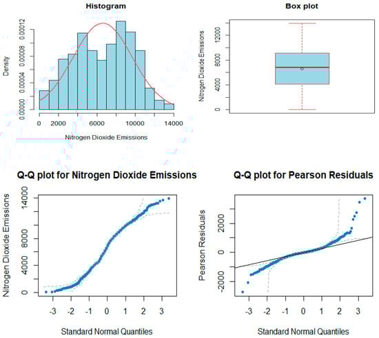
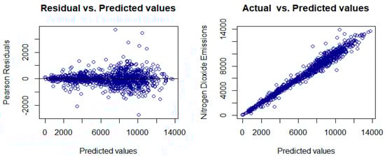
Figure 5. The histogram (top left), Box plot (top right), Q-Q plots for NO₂ emissions (tons) (middle left) and Q-Q plots for raw residuals from regression analysis (middle right), and the plot of residuals versus predicted values (bottom left) and observed values versus predicted values (bottom right), for both the linear regression model.

In Figure 5, the histogram of the original data (NO₂ emissions) appears to have an asymmetrical shape and is bimodal, indicating a departure from a Normal distribution (Kolmogorov–Smirnov p-value < 0.01). Additionally, the Box plot of the same data reveals some skewness (with a value of −0.11) and kurtosis (with a value of −0.94) in NO₂ emissions (in tons).

The Q-Q plots of the original data against Normal distribution quantiles indicate that NO₂ emissions (in tons) are not Normally distributed, as the data points deviate from the 45° line in the graph’s extremities. The QQ plot of the NO₂ emissions data against the Normal quantiles also indicates that the data are not Normally distributed as the plot is not linear. The Pearson residuals from the regression line also indicate that the model is not a good fit as the Normality assumption (${\epsilon }_{tp}~N(0,{\sigma }^2)$ is not met. The QQ plot of the resultant residuals and Normal quantiles is not linear. It can be concluded that NO₂ emissions (in tons) do not follow a Normal distribution based on the plots in Figure 5. Additionally, in the plots in the last row of Figure 5, the Normal distribution model (regression analysis), given by Equation (18), seems to suggest an increasing variance with the predicted values; hence, the model is not very good. Consequently, the Lognormal and Loggamma distributions are fitted to try and tame the variance.

Figure 6 below shows the plot of residuals versus predicted values and observed values versus predicted values for both the Lognormal and Loggamma distribution models. The plots are used to compare and assess the goodness of fit of the models.

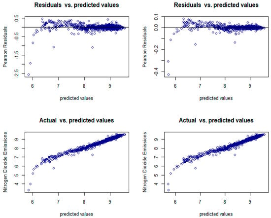
Figure 6. Residuals against the predicted values of the Lognormal (top left) and Loggamma (top right) distribution models and the actual against predicted value plots for the Lognormal (bottom left) and Loggamma (bottom right) distribution models, both with the identity link function.

In the plot of the observed against predicted values in Figure 6, the Lognormal and Loggamma distribution models with the identity link function produced a plot with a somewhat constant variance over the predicted values; hence, the models give a good fit.

To confirm the best link function within each of the distribution models, the deviance is compared to the degrees of freedom (df). Generally, a model with a smaller deviance is preferred [28,29]. A model with a value of $deviance/df <1$ suggests a good model fit, while a model with $deviance/df >1$ suggests a poor model fit [28,29,49]. For the Normal distribution, however, the deviance cannot be used as a direct goodness-of-fit statistic due to its dependence on $Var\left(Y_i\right)={\sigma }^2$ [49]. Table 4 shows the model used, the deviance, and the degrees of freedom for both the Lognormal and Loggamma distribution models. Three link functions, namely, the identity, log, and inverse functions, are considered to determine the most suited one for the data in each the distribution models.

Table 4. Deviances and degrees of freedom.

Distribution Model	Degrees of Freedom	Deviance
		Identity	Log	Inverse
Lognormal	1257	24.0395	26.1316	28.0781
Loggamma	1257	0.6555	0.7131	0.7632

The Lognormal and Loggamma distribution models both produced good fits to the NO₂ emissions data, and they have deviance values that are smaller than their associated degrees of freedom, with a value of $deviance/df <1$ across the three link functions. The identity link function gave the lowest deviance for the two distribution models in this study and was hence used.

To measure the model adequacy of the Lognormal and Loggamma GLM based distribution models, two related performance indicators are used, namely, the variance-function-based R² and the adjusted R². The classical R², which assumes normality of data, is well defined for GLMs with homoscedastic residuals, while the likelihood based R², e.g., R² by Magee [50], Maddala [51], Cox and Snell [52], and Nagelkerke [53], and the KL-divergence-based R² by Cameron and Windmeijer [54], require a well-defined likelihood function. However, the variance-function-based R² and the adjusted R² by Zhang [55] take into account the relationship between the mean and variance functions and do not require the likelihood function in their computation [55], making them particularly a good choice for the current study. Table 5 presents the variance-function-based R² and the adjusted R² for the Lognormal and Loggamma distributions.

Table 5. Variance-function-based R² for the Lognormal and Loggamma distributions.

Distribution Model	Variance-Function-Based Measure
	R2	Adjusted R2
Lognormal	0.9605	0.9593
Loggamma	0.9711	0.9703

In Table 5, both the Lognormal and Loggamma distributions demonstrate a good fit, with all the performance indicators giving very similar values. For example, both distribution models have an R² value that is very close to 1, with R² = 0.9605 for the Lognormal model and R² = 0.9711 for the Loggamma model. However, it can be noted that the Loggamma distribution model gave better results than the Lognormal distribution model for both measures (R² and adjusted R²).

5. Discussion

The performance of the GLM-based Loggamma distribution model is compared with that of the traditional Normal distribution based simple linear regression model and the GLM-based Lognormal. The Normal distribution model assumes a constant variance in modelling NO₂ emissions from Eskom’s 13 coal-fuelled power stations in South Africa. In essence, this study investigates whether log transforming the NO₂ emission data and fitting two GLM based models, i.e., the Normal and the Gamma models, can give a good fit if the assumption of normality of the data does not hold.

The ordinary least squares method is used to estimate the parameters of the regression model. The results of the linear regression model suggest that NO₂ emissions data are not Normally distributed, which is also supported by the results of the histogram, Box plot, and QQ plots. The very large deviance value compared to the degrees of freedom in the Normal model also suggested that the linear regression model does not give a good fit when modelling the NO₂ emissions data. The assumption of Normality of the data does not hold and thus, one cannot obtain a good fitting model to the data when using a linear regression model. This does not come as a surprise since it is common to find emissions data, including NO₂, that violate the Normality assumption [17,18,19,20,21,22,56,57,58], especially when the variance increases with the mean [36].

MLE parameter estimation methods were used for the GLM distribution models. The results indicate that the Lognormal and Loggamma models, both with the identity link function, gave a good fit, with the Loggamma producing a better fit between the two. These finding suggest that the GLM with the Loggamma distribution model provides a better framework for predicting NO₂ emissions from coal-fuelled power stations at Eskom. Therefore, Loggamma distribution models can carter to increasing variance with the predicted values (see Figure 6).

Of the two distributions, the Lognormal distribution is common in applications of pollutant emission [59,60,61,62,63], although it is less prevalent in a GLM framework for modelling NO₂ emissions from coal-fired power stations. There is little if any evidence of the Loggamma distribution’s application in NO₂ emission modelling from coal-fired power stations, especially in a GLM setup. Thus, the current study uses these GLM distribution models to close the gap and better explain NO₂ emissions data patterns.

The model is able to capture and quantify the behaviour of NO₂ emissions, as well as capture the important or significant variables, such as electricity sent out (in GWhs), age of the power station (in years), and power station used, and the interaction terms, such as electricity × station and age × station. High- and low-emission stations are identified, e.g., the power stations Kendal, Komati, and Tutuka are flagged by the parameter estimates for the terms “power station”, “electricity × station”, and “age × station”, respectively, as having the largest effect on increasing emissions, while Arnot, Kendal, and Komati are flagged as having the lowest effect.

Based on mean relative emissions, the abatement technologies associated with the lowest and highest emissions are also identified, with the joint fabric filter and electrostatic precipitators, along with flue gas conditions, exhibiting the highest efficiency, while the electrostatic precipitators demonstrated the highest efficiency.

All the above information can be used to formulate concrete air pollution mitigation strategies, such as identifying which power station should get a new abatement technology. The information provided by the model can be used to meet regulations and adherence, promoting sustainability in the energy sector.

Therefore, Eskom can use the methods applied in this study to understand similar other power plants and environments not considered herein. The Loggamma model method employed here has not received wide and significant attention in the field of emissions modelling.

Air pollution from industrial areas can be managed and regulated. This includes areas such as coal-fired power stations. To achieve this, statistical information is needed to influence decisions and regulations that need to be enforced. In a developing country such as South Africa, economic growth is very important, but this should not come at the expense of our health and the environment. Striking a balance is a challenge. While the country strives to promote eco-friendly power generation, the energy demand keeps rising, compelling Eskom to prolong the operation of aged coal power stations and the postponement of their permanent decommissioning in order to meet current demand. Statistical models such as the Loggamma model proposed here can help quantify emissions to understand how long we can delay the inevitable closure of some of these power plants. Stringent policy and management strategies for reducing and mitigating emissions should be informed by models such as the Loggamma. Our results suggest prioritising the electricity sent out, the age of a power station, and/or least efficient power stations as a starting point while accelerating renewable energy efforts.

Recommendation

The findings of the current study demonstrate the benefits in deriving information on emissions by fitting the Loggamma distribution over the Normal distribution in a GLM setup when the data are non-Normal and the variance increases with the mean. The Loggamma distribution is a somewhat heavy tailed distribution, akin to the Lognormal distribution. The Lognormal distribution is in the Gumbel domain of attraction, but the Loggamma is in the Pareto-type [32] heavier tail. The findings indicate the potential presence of extremes in the data. As a result, the next stage will be to investigate the tail distribution of the NO₂ emissions from Eskom’s coal-fuelled power stations by exploring extreme value theory distributions, namely, the generalised extreme value distribution (GEVD) and the generalised Pareto distribution (GPD). This is crucial for understanding the frequency and intensity of extremely high NO₂ emissions events and can provide information for more targeted mitigation strategies for the most severe air pollution scenarios and the power stations responsible for such high emissions. This is especially relevant considering the exacerbated effects of environmental and human exposure to very high NO₂ emissions.

6. Conclusions

This paper fitted and compared three GLM distribution models, namely, the Normal, Lognormal, and Loggamma distribution models, with the identity link function in the modelling of NO₂ emissions at Eskom’s 13 coal-fuelled power stations. Through backward stepwise variable selection, two predictive models were developed, representing the two distributions. The NO₂ emissions data have a variance that increases with the mean of the emissions. The residual plots, actual versus predicted plots, and deviance values (against their associated degrees of freedom) confirm the best fit of the Loggamma model to the NO₂ emissions data over the Normally distributed based regression model and the Lognormal GLM.

These results are significant for understanding and predicting NO₂ emissions, particularly when considering electricity production from Eskom’s coal-fuelled power stations in South Africa. Using the Loggamma-distributed GLM model for NO₂ emissions, the emissions can be explained and predicted. This will assist in developing effective strategies to lower air pollution and promote sustainable practices in the energy industry.

The application of these models to other emissions, geographical locations, and power generation facilities can provide valuable information on the generalisability and applicability of the findings. Overall, this study contributes to the modelling technique enhancement for NO₂ emissions and provides useful information for policymakers and stakeholders involved in air quality management and energy production, especially in the case of Eskom in South Africa.

References

- Dadhich, A.P.; Goyal, R.; Dadhich, P.N. Assessment of Spatio-Temporal Variations in Air Quality of Jaipur City, Rajasthan, India. Egypt. J. Remote Sens. Space Sci. 2018, 21, 173–181. [Google Scholar] [CrossRef]
- Tandon, A.; Yadav, S.; Attri, A.K. City-Wide Sweeping a Source for Respirable Particulate Matter in the Atmosphere. Atmos. Environ. 2008, 42, 1064–1069. [Google Scholar] [CrossRef]
- Guerreiro, C.B.B.; Foltescu, V.; de Leeuw, F. Air Quality Status and Trends in Europe. Atmos. Environ. 2014, 98, 376–384. [Google Scholar] [CrossRef]
- Samoli, E.; Aga, E.; Touloumi, G.; Nisiotis, K.; Forsberg, B.; Lefranc, A.; Pekkanen, J.; Wojtyniak, B.; Schindler, C.; Niciu, E.; et al. Short-Term Effects of Nitrogen Dioxide on Mortality: An Analysis within the APHEA Project. Eur. Respir. J. 2006, 27, 1129–1138. [Google Scholar] [CrossRef]
- Tschoeke, H.; Mollenhauer, K. Handbook of Diesel Engines; Springer: Berlin/Heidelberg, Germany; Dordrecht, The Netherlands; London, UK; New York, NY, USA, 2010. [Google Scholar] [CrossRef]
- Anand, S.; Varma, K.; Srimurali, M. Concentration of Nitrogen Dioxide Estimation from Modeled NOX of a Thermal Power Plant. J. Environ. Sci. Toxicol. Food Technol. 2013, 6, 08–11. [Google Scholar]
- Longhurst, J.W.S.; Lindley, S.J.; Watson, A.F.R.; Conlan, D.E. The Introduction of Local Air Quality Management in the United Kingdom: A Review and Theoretical Framework. Atmos. Environ. 1996, 30, 3975–3985. [Google Scholar] [CrossRef]
- Nagendra, S.M.S.; Khare, M. Artificial Neural Network Approach for Modelling Nitrogen Dioxide Dispersion from Vehicular Exhaust Emissions. Ecol. Modell. 2006, 190, 99–115. [Google Scholar] [CrossRef]
- Sharma, P.; Chandra, A.; Kaushik, S.; Sharma, P.; Jain, S. Predicting Violations of National Ambient Air Quality Standards Using Extreme Value Theory for Delhi City. Atmos. Pollut. Res. 2012, 3, 170–179. [Google Scholar] [CrossRef][Green Version]
- Khare, M.; Sharma, P. Modelling Urban Vehicle Emissions; WIT Press: Southampton, UK, 2002. [Google Scholar][Green Version]
- Dai, H.; Huang, G.; Zeng, H. Multi-Objective Optimal Dispatch Strategy for Power Systems with Spatio-Temporal Distribution of Air Pollutants. Sustain. Cities Soc. 2023, 98, 104801. [Google Scholar] [CrossRef]
- Dai, H.; Huang, G.; Wang, J.; Zeng, H. VAR-Tree Model Based Spatio-Temporal Characterization and Prediction of O3 Concentration in China. Ecotoxicol. Environ. Saf. 2023, 257, 114960. [Google Scholar] [CrossRef] [PubMed]
- Bencala, K.E.; Seinfeld, J.H. On Frequency Distributions of Air Pollutant Concentrations. Atmos. Environ. 1976, 10, 941–950. [Google Scholar] [CrossRef] [PubMed]
- Georgopoulos, P.G.; Seinfeld, J.H. Statistical Distributions of Air Pollutant Concentrations. Environ. Sci. Technol. 1982, 16, 401A–416A. [Google Scholar] [CrossRef]
- Lu, H.-C. Estimating the Emission Source Reduction of PM10 in Central Taiwan. Chemosphere 2004, 54, 805–814. [Google Scholar] [CrossRef]
- Hogg, R.V.; Klugman, S.A. Loss Distributions; John Wiley & Sons: Hoboken, NJ, USA, 1984. [Google Scholar]
- Hadley, A.; Toumi, R. Assessing Changes to the Probability Distribution of Sulphur Dioxide in the UK Using a Lognormal Model. Atmos. Environ. 2003, 37, 1461–1474. [Google Scholar] [CrossRef]
- Rumburg, B.; Alldredge, R.; Claiborn, C. Statistical Distributions of Particulate Matter and the Error Associated with Sampling Frequency. Atmos. Environ. 2001, 35, 2907–2920. [Google Scholar] [CrossRef]
- Kao, A.S.; Friedlander, S.K. Frequency Distributions of PM10 Chemical Components and Their Sources. Environ. Sci. Technol. 1995, 29, 19–28. [Google Scholar] [CrossRef] [PubMed]
- Mijić, Z.; Tasić, M.; Rajšić, S.; Novaković, V. The Statistical Characters of PM10 in Belgrade Area. Atmos. Res. 2009, 92, 420–426. [Google Scholar] [CrossRef]
- Morel, B.; Yeh, S.; Cifuentes, L. Statistical Distributions for Air Pollution Applied to the Study of the Particulate Problem in Santiago. Atmos. Environ. 1999, 33, 2575–2585. [Google Scholar] [CrossRef]
- Zhang, Y.; Bishop, G.A.; Stedman, D.H. Automobile Emissions Are Statistically Gamma Distributed. Environ. Sci. Technol. 1994, 28, 1370–1374. [Google Scholar] [CrossRef]
- Sahsuvaroglu, T.; Arain, A.; Kanaroglou, P.; Finkelstein, N.; Newbold, B.; Jerrett, M.; Beckerman, B.; Brook, J.; Finkelstein, M.; Gilbert, N.L. A Land Use Regression Model for Predicting Ambient Concentrations of Nitrogen Dioxide in Hamilton, Ontario, Canada. J. Air Waste Manag. Assoc. 2006, 56, 1059–1069. [Google Scholar] [CrossRef] [PubMed]
- Boznar, M.; Lesjak, M.; Mlakar, P. A Neural Network-Based Method for Short-Term Predictions of Ambient SO2 Concentrations in Highly Polluted Industrial Areas of Complex Terrain. Atmos. Environ. Part B Urban Atmos. 1993, 27, 221–230. [Google Scholar] [CrossRef]
- Gardner, M.; Dorling, S.R. Neural Network Modelling and Prediction of Hourly NOx and NO2 Concentrations in Urban Air in London. Atmos. Environ. 1999, 33, 709–719. [Google Scholar] [CrossRef]
- Comrie, A.C. Comparing Neural Networks and Regression Models for Ozone Forecasting. J. Air Waste Manag. Assoc. 1997, 47, 653–663. [Google Scholar] [CrossRef]
- Dobson, A.J.; Barnett, A.G. An Introduction to Generalized Linear Models, 3rd ed.; Carlin, B.P., Faraway, J.J., Tanner, M., Zidek, J., Eds.; Texts in Statistical Science Series; CHAPMAN & HALL/CRC: New York, NY, USA, 2008. [Google Scholar]
- Myers, R.H.; Montgomery, D.C.; Vining, G.G.; Robinson, T.J. Generalized Linear Models: With Applications in Engineering and the Sciences; John Wiley & Sons: Hoboken, NJ, USA, 2010. [Google Scholar]
- de Jong, P.; Heller, G.Z. Generalized Linear Models for Insurance Data; Cambridge University Press: Cambridge, UK, 2008. [Google Scholar]
- Lee, D.K. Data Transformation: A Focus on the Interpretation. Korean J. Anesthesiol. 2020, 73, 503–508. [Google Scholar] [CrossRef]
- Embrechts, P.; Kluppelberg, C.; Mikosch, T. Modelling Extremal Events for Insurance and Finance; Springer: Berlin/Heidelberg, Germany, 1997. [Google Scholar]
- Albrecher, H.; Beirlant, J.; Teugels, J.L. Reinsurance: Actuarial and Statistical Aspects; John Wiley & Sons: Hoboken, NJ, USA, 2017. [Google Scholar]
- Ramlau-Hansen, H. A Solvency Study in Non-Life Insurance. Scand. Actuar. J. 1988, 1988, 3–34. [Google Scholar] [CrossRef]
- Box, G.E.P.; Cox, D.R. An Analysis of Transformations. J. R. Stat. Soc. Ser. B 1964, 26, 211–243. [Google Scholar] [CrossRef]
- Lindsey, J. Applying Generalized Linear Models; Text in Statistics; Springer: Berlin/Heidelberg, Germany, 1997. [Google Scholar]
- McCullagh, P.; Nelder, J.A. Generalized Linear Models, 2nd ed.; Chapman and Hall: London, UK, 1989. [Google Scholar]
- Hardin, J.; Hilbe, J. Generalized Linear Models and Extensions, 2nd ed.; StrataCorp LP: College Station, TX, USA, 2007. [Google Scholar]
- Eskom. Eskom-Partnering for a Sustainable Future, Integrated Report 2011. 2011. Available online: https://www.eskom.co.za/wp-content/uploads/2021/10/eskom-ar2011.pdf (accessed on 29 July 2025).
- Morosele, I.P.; Langerman, K.E. The Impacts of Commissioning Coal-Fired Power Stations on Air Quality in South Africa: Insights from Ambient Monitoring Stations. Clean Air J. 2020, 30. [Google Scholar] [CrossRef]
- Pretorius, I.; Piketh, S.; Burger, R.; Neomagus, H. A Perspective on South African Coal Fired Power Station Emissions. J. Energy S. Afr. 2015, 26, 27–40. [Google Scholar] [CrossRef]
- Mukherjee, A.; Agrawal, M. Use of GLM Approach to Assess the Responses of Tropical Trees to Urban Air Pollution in Relation to Leaf Functional Traits and Tree Characteristics. Ecotoxicol. Environ. Saf. 2018, 152, 42–54. [Google Scholar] [CrossRef]
- Shah, M.A.A.; Özel, G.; Chesneau, C.; Mohsin, M.; Jamal, F.; Bhatti, M.F. A Statistical Study of the Determinants of Rice Crop Production in Pakistan. Pakistan J. Agric. Res. 2020, 33, 97–105. [Google Scholar] [CrossRef]
- Musood, T.; Kaur, B. The Mediating Role of Mindful Attention Awareness in the Relationship Between Self-Esteem and Cognitive Flexibility Among Pre-Service Teachers. MIER J. Educ. Stud. Trends Pract. 2025, 15, 76–98. [Google Scholar] [CrossRef]
- Zahoor, Z.; Shahzad, K.; Mustafa, A.U. Do Climate Changes Influence the Agriculture Productivity in Pakistan? Empirical Evidence from ARDL Technique. Forman J. Econ. Stud. 2022, 18, 97–116. [Google Scholar] [CrossRef]
- UYAK, V.; OZDEMIR, K.; TOROZ, I. Multiple Linear Regression Modeling of Disinfection By-Products Formation in Istanbul Drinking Water Reservoirs. Sci. Total Environ. 2007, 378, 269–280. [Google Scholar] [CrossRef] [PubMed]
- Kumari, M.; Gupta, S.K. Modeling of Trihalomethanes (THMs) in Drinking Water Supplies: A Case Study of Eastern Part of India. Environ. Sci. Pollut. Res. 2015, 22, 12615–12623. [Google Scholar] [CrossRef]
- Montgomery, D.C.; Peck, E.A.; Vining, G.G. Introduction to Linear Regression Analysis, 5th ed.; Balding, D.J., Cressie, N.A.C., Fitzmaurice, G.M., Goldstein, H., Johnstone, I.M., Molenberghs, G., Scott, D.W., Smith, A.F.M., Tsay, R.S., Weisberg, S., Eds.; John Wiley & Sons, Inc.: Hoboken, NJ, USA, 2012. [Google Scholar]
- Eskom. As Komati Coal-Fired Power Station Reaches End of Life, Renewable Energy Project Takes Shape. Available online: https://www.eskom.co.za/as-komati-coal-fired-power-station-reaches-end-of-life-renewable-energy-project-takes-shape/ (accessed on 24 June 2024).
- Dobson, A.J. An Introduction to Generalized Linear Models, 2nd ed.; Chapman & Hall/CRC: Boca Raton, FL, USA, 2002. [Google Scholar]
- Magee, L. R2 Measures Based on Wald and Likelihood Ratio Joint Significance Tests. Am. Stat. 1990, 44, 250–253. [Google Scholar] [CrossRef]
- Maddala, G.S. Limited-Dependent and Qualitative Variables in Econometrics; Cambridge University Pree: Cambridge, UK, 1983. [Google Scholar]
- Cox, D.R.; Snell, E.J. The Analysis of Binary Data, 2nd ed.; Chapman and Hall: London, UK, 1989. [Google Scholar]
- NAGELKERKE, N.J.D. A Note on a General Definition of the Coefficient of Determination. Biometrika 1991, 78, 691–692. [Google Scholar] [CrossRef]
- Colin Cameron, A.; Windmeijer, F.A.G. An R-Squared Measure of Goodness of Fit for Some Common Nonlinear Regression Models. J. Econom. 1997, 77, 329–342. [Google Scholar] [CrossRef]
- Zhang, D. A Coefficient of Determination for Generalized Linear Models. Am. Stat. 2017, 71, 310–316. [Google Scholar] [CrossRef]
- Aydin, D. A Comparison of the Statistical Distributions of Air Pollution Concentrations in Sinop, Turkey. Environ. Prot. Eng. 2024, 50, 47–68. [Google Scholar] [CrossRef]
- Bağci, K. Application of Statistical Distributions to PM10 Concentrations: Van, Türkiye. Yüzüncü Yıl Üniversitesi Sos. Bilim. Enstitüsü Derg. 2023, 60, 87–95. [Google Scholar] [CrossRef]
- De Souza, A.; Olaofe, Z.O.; Kodicherla, S.P.K.; Ikefuti, P.; Nobrega, L.; Sabbah, I. Probability Distributions Assessment for Modeling Gas Concentration in Campo Grande, MS, Brazil. Eur. Chem. Bull. 2018, 6, 569. [Google Scholar] [CrossRef][Green Version]
- Aleksandropoulou, V.; Eleftheriadis, K.; Diapouli, E.; Torseth, K.; Lazaridis, M. Assessing PM 10 Source Reduction in Urban Agglomerations for Air Quality Compliance. J. Environ. Monit. 2012, 14, 266–278. [Google Scholar] [CrossRef] [PubMed]
- Mishra, G.; Ghosh, K.; Dwivedi, A.K.; Kumar, M.; Kumar, S.; Chintalapati, S.; Tripathi, S.N. An Application of Probability Density Function for the Analysis of PM2.5 Concentration during the COVID-19 Lockdown Period. Sci. Total Environ. 2021, 782, 146681. [Google Scholar] [CrossRef]
- Gao, C.; Deng, S.; Jiang, X.; Guo, Y. Analysis for the Relationship Between Concentrations of Air Pollutants and Meteorological Parameters in Xi’an, China. J. Test. Eval. 2016, 44, 1064–1076. [Google Scholar] [CrossRef]
- Gulia, S.; Nagendra, S.M.S.; Khare, M. Extreme Events of Reactive Ambient Air Pollutants and Their Distribution Pattern at Urban Hotspots. Aerosol Air Qual. Res. 2017, 17, 394–405. [Google Scholar] [CrossRef]
- Hrishikesh, C.G.; Nagendra, S.M.S. Study of Meteorological Impact on Air Quality in a Humid Tropical Urban Area. J. Earth Syst. Sci. 2019, 128, 118. [Google Scholar] [CrossRef]
Disclaimer/Publisher’s Note: The statements, opinions and data contained in all publications are solely those of the individual author(s) and contributor(s) and not of MDPI and/or the editor(s). MDPI and/or the editor(s) disclaim responsibility for any injury to people or property resulting from any ideas, methods, instructions or products referred to in the content. |
© 2025 by the authors. Licensee MDPI, Basel, Switzerland. This article is an open access article distributed under the terms and conditions of the Creative Commons Attribution (CC BY) license (https://creativecommons.org/licenses/by/4.0/).