Retrieval of Long-Term (1980–2024) Time Series of PM10 Concentration by an Empirical Method: The Paris, Cairo, and New Delhi Case Studies

Abstract

Pluriannual time series of fine particle concentrations suspended in the atmosphere are often lacking. Such data is necessary in evaluating the efficiency of policies aiming to improve air quality in megacities. In this work, a recently developed empirical method is applied over the megacities of Paris, Cairo, and New Delhi. The method utilizes observations of the aerosol optical depth, Angström Exponent, and atmospheric precipitable water as inputs to estimate the PM10. The modeled values validated against their respective reference measurements exhibited the best performance at daily, weekly, and monthly averages when using inputs of the AERONET. When exploiting inputs of the CAMS and MERRA-2 reanalyses, the results were found to be satisfactory with MERRA-2 on the monthly scale. This allows the reconstruction of the variability of the PM10 for the last 45 years. Analysis shows that average annual PM10 concentration has decreased from 40 to 20 µg·m⁻³ in Paris, increased from 70 to 250 µg·m⁻³ in New Delhi, and stayed relatively stable (around 100 µg·m⁻³) in Cairo. Provided that at least one year of PM10 measurements are available to calibrate the empirical method, the method herein is replicable over other megacities around the world.

1. Introduction

Human activities, such as the burning of fossil fuels for industry and transport, agriculture, and land use change, deeply modify the composition of the atmosphere of the earth. The increase in the concentration of noxious species in the atmosphere due to such activities is referred to as air pollution. The effects of the anthropogenic emissions of greenhouse gases (GHGs) on climate change are well documented [1]. Public health and the environment are also seriously threatened by air-suspended particulate matter (PM), and by gaseous species such as nitrogen oxides (NO_x), ground-level ozone (O₃), sulfur dioxide (SO₂), carbon monoxide (CO), or volatile organic compounds (VOCs). Indeed, the World Health Organization (WHO) estimates that air pollution causes around 7 million premature deaths annually, mostly from respiratory and cardiovascular diseases, strokes, and lung cancer [2]. Beyond mortality, air pollution also has a direct impact on morbidity: lung and bloodstream penetration of particles with aerodynamic diameters finer than 2.5 µm (PM2.5) aggravates conditions including asthma, chronic obstructive pulmonary disease (COPD), and ischemic heart disease [3].

Vegetation is also affected by SO₂, NO₂, and O₃, and the deposition of PM on the leaves leads to substantial yield loss [4]. At regional and global scales, the anthropogenic modification of the composition of the soils, aquatic environments, and forests contributes to the current dramatic reduction in biodiversity [5].

In the lower troposphere, the atmospheric lifetime of the pollutants considered as most harmful for human health and the environment hardly exceeds a week [6]. Therefore, their concentrations are the largest in the vicinity of the sources, which are essentially located in urbanized regions. Because of the accelerated industrialization, increased vehicle emissions, and rapid urban growth, air pollution has become a major matter of concern in megacities, and particularly those of the developing world [7,8]. Addressing these issues calls for regulatory initiatives. To lower particulate matter emissions, governments tend to pass stricter regulations for car, household, and industrial emissions. For instance, this was the objective of the revised Ambient Air Quality Directive in the European Union (EU) [9] and the European Environment Agency (EEA) [10]. Also, the United States Environmental Protection Agency recently revised the National Ambient Air Quality Standards for fine particulate matter [11]. At smaller spatial scales, cities also try to lower their pollution levels by setting low-emission zones, strengthening networks of air quality monitoring, and pushing greener energy options [12]. Reducing PM pollution and promoting sustainable urban life depend critically on investments in green infrastructure, improved public transportation, and stricter air quality rules.

In the 27 member states of the EU, the benefits of these efforts have been quantified by the EEA: the number of deaths attributable to PM2.5 has fallen by 41% between 2005 and 2021. Nonetheless, in 2021, the PM, NO₂, and O₃ concentrations were still well above the air quality guidelines of the WHO. With 432,000 attributable deaths that year, the PM represented a larger health hazard than NO₂ and O₃, amounting to 232,000, 142,000 and 108,000 deaths, respectively [13].

In 2020 and 2021, the COVID-19 pandemic lockdowns implemented in many countries worldwide constituted a real-life experiment to evaluate the efficiency of forced short-term restrictions of activity. Because of the limitation of motorized traffic, concentrations of NO₂ in the atmosphere dropped significantly [14]. Globally, PM2.5 also tended to decrease [15], but a study focusing on 28 European locations [16] suggested that no significant reduction in the PM2.5 concentration could be associated with the implementation of the lockdowns in urban sites. Peaks of PM2.5 concentrations were even observed in Paris during the spring 2020 lockdown. They were attributed to agricultural activities in the fields surrounding the Parisian conurbation [17]. For O₃, the results were also contrasted: an increase in the concentration was observed in most megacities because of the reduction in the nocturnal sink associated with NO_x [18,19]. However, O₃ concentrations decreased in the megacities of southern China [20] and in the Greater Cairo area in Egypt [21]. In the first case, meteorological factors and reduced emissions of VOCs, which are precursors of ozone, might explain the decrease. In the second one, the authors hypothesize that air-suspended mineral dust might act as an ozone sink compensating for the limitation of nocturnal titration by the NO_x.

These examples show that complex factors of different natures control the short-term variations in the concentrations of pollutants, which makes it difficult to evaluate the actual efficiency of mitigation strategies from measurements made over limited durations. Ideally, this evaluation should be based on the analysis of datasets of concentrations measured in situ and spanning several years, if not decades. Unfortunately, consistent and reliable air pollution datasets are often unavailable, or insufficiently broad in many regions, particularly in developing megacities, to support meaningful long-term assessments [22,23].

As substitutes to time series of data of direct measurements, different approaches were proposed in the literature to estimate ground-level concentrations of pollutants, especially PM, which has the highest health burden. In their review of these approaches, Shin et al. [24] proposed to distinguish the methods based on chemical transport models (CTMs) from the empirical-statistical ones, which try to derive the surface concentrations from remote sensing observations.

When coupled with reanalyzed meteorological products, the CTMs can simulate the fate of air-suspended particles from their emission (or production) to their final removal from the atmosphere. This method yields historical datasets of concentrations such as those of the Copernicus Atmosphere Monitoring Service (CAMS) of the European Centre for Middle-Range Weather Forecasts (ECMWF) [25,26] or of the Modern-Era Retrospective analysis for Research and Applications, Version 2 (MERRA-2) of the National Aeronautics and Space Administration (NASA) [27]. The shortcomings of these reanalysis datasets arise from possible mistakes in meteorological data, emission inventories, and atmospheric chemical interactions [28].

Empirical methods use remote sensing products, generally the Aerosol Optical Depth (AOD), and their statistical relationships with observed surface particulate matter concentrations to produce models of varying complexities. These approaches include multiple linear regression (MLR) and machine learning models such as random forests and neural networks [29,30]. Because of their computational efficiency, these models are widely used in air-quality applications, but their training requires extensive datasets. Also, because of their purely statistical nature, they are black-box models with unknown considerations of the complex atmospheric interactions [31,32].

Based on the laws of physics, which imply that the relationship between the AOD and the surface PM concentration should depend on the nature (size, chemical composition and hydrophilic character) of the aerosols as well as on their vertical distribution in the atmospheric column, vertical correction models were proposed. Among these, the simplest models use only the planetary boundary layer height (H) and relative humidity (RH) to modify the AOD/surface–concentration relationship, and thus improve the estimate of surface-level PM concentrations [33,34]. More recently, Said et al. [35] proposed an empirical retrieval of the surface PM10 concentration (hereinafter simply referred to as C) based on co-located observations performed by the sunphotometers of the Aerosol Robotics Network (AERONET) [36,37,38] Beside the AOD at several wavelengths, these observations include the columnar content in precipitable water (PW), and they allow the calculation of the Ångström exponent (AE). The AE quantifies the spectral dependence of the AOD [36,39] and is deeply related to the size-distribution of the air-suspended particles, which makes of it a good proxy of the aerosol type. Said et al. [35] applied their new parameterizing technique to estimate surface PM10 concentrations in Cairo and New Delhi and showed that, with correlation coefficients exceeding 0.81, their method was effective in retrieving PM10 readings at the weekly and monthly temporal resolutions. Particularly in New Delhi, where aerosols showed heightened hygroscopic properties, the study found that variations in PW greatly affected the correlation between the AOD and the PM10 surface concentration. Seasonal fluctuations in aerosol composition—including spring dust storms in Cairo—were satisfyingly considered by the means of the AE, which had a notable influence on the AOD-PM10 correlation. Finally, other vertical correction methods, such as H in the parameterization, improved the accuracy of the model.

In view of these good performances, the first question to arise is that of the added value of this new method: does the empirical method really perform better than the products of the most widely used reanalyses? The second question is related to the availability of AERONET measurements. Indeed, despite the efforts of the scientific community to develop its network of instruments, many megacities are still not equipped with AERONET stations. In this case, how does the empirical method perform if input data derived from satellite observations or provided by reanalyses are used?

The objective of this work is to assess the performance of the method of Said et al. to estimate the PM10 concentration over three megacities, and to compare that with the estimates of reanalysis data. Three megacities were selected for having contrasting climates, and assumedly quite different types of aerosols: Cairo, Paris, and New Delhi. The method is then applied to reconstruct multidecadal time series of the surface PM10 concentration in these megacities.

The structure of the paper is as follows: Section 2 first summarizes the principles of the method proposed by Said et al. [35] (hereinafter more simply referred to as S2023), then alternative inputs that could be used as substitutes to missing AERONET data are identified. The selected locations and the observational data collected are then presented, followed by the reanalysis products to which the empirical retrievals will also be compared. Finally, the metrics employed for the quantification of the accuracy of the method are described. In the results and discussion (Section 3), the outputs of S2023 when using AERONET data are first compared with those of the MERRA-2 and CAMS reanalyses, then the modification of the predictions of S2023 when substitute inputs are used instead of the AERONET ones are quantified. A thorough discussion of these results follows. The final conclusions of the study are drawn in Section 4.

2. Data and Methods

2.1. Model of Said et al.

In S2023, the two main assumptions underlying the derivation of the surface concentration of PM10 from the AOD measured by the sunphotometer were that (1) the bulk of the atmospheric aerosols was located inside the planetary boundary layer (PBL), which is tantamount to considering that the transport of particles outside the PBL is rather the exception than the rule, and (2) this concentration was homogenous. This led to a very simple relationship between the AOD and the mean concentration (C_mean) within the PBL:

AOD = C_mean σ H

(1)

In this expression, σ (usually expressed in m²·g⁻¹) represents the mass extinction efficiency of the aerosols at the same wavelength (in this work, λ = 550 nm) as the AOD. It depends on the physical characteristics (size, shape, hygroscopicity) and composition of the air-suspended particles. Therefore, it usually varies with the nature of these particles, and as a result of their interactions with atmospheric humidity. In other words, the AOD/C_mean ratio is not constant. Using AE as a proxy of the size of the aerosols, PW (in mm) as one of atmospheric humidity, and making a first order development around the mean values of the parameters of influence, Said et al. [35] obtained

$$AOD/C_{mean}={\sigma }_{mean}{H}_{mean} (1+C1(AE-{AE}_{mean}\left)\right)(1+C2(PW-{PW}_{mean}\left)\right)(1+C3(H-H_{mean}\left)\right)$$

(2)

However, recent measurements of the PM concentration at different altitudes within the PBL revealed that the vertical profiles of profiles are not necessarily homogenous [40]: depending on meteorological conditions and the hour of the day, the concentration at the surface (C) can be larger, smaller, or comparable to that of the rest of the PBL. In other words, C is usually related to C_mean, but not strictly equal to it. The simplest way of expressing this correlation is to estimate that the concentration at the surface is proportional to C_mean. The proportionality constant (k) is equal to one when the concentration profile is homogenous, as assumed by Said et al., but it can also be larger or smaller depending on the situation. This leads to a slightly modified version of Equation (2):

$$AOD/C=({k\sigma H)}_{mean} (1+C1(AE-{AE}_{mean})\left)\right(1+C2(PW-{PW}_{mean})\left)\right(1+C3(H-H_{mean}))$$

(3)

The coefficients C1, C2, and C3 quantify the sensitivity of the AOD/C ratio to variations around the mean values of AE, PW, and H, respectively. C1 is unitless, C2 in mm⁻¹, and C3 in m⁻¹. Their unknown values and those of the mean of the kσH product are yielded by an iterative least square routine (LSR) providing the best fit of Equation (3) to the daily values of the AOD/C ratio measured at the experimental sites. Because only daily values are used in the adjustment, the impact of the hour-to-hour variations in k is most probably smoothed by the temporal averaging. This will be even more the case when larger (weekly or monthly) temporal resolutions will be considered. Also, note that before application of the LSR, the outliers in the statistical distribution of the AOD/C ratio were discarded because they could correspond to cases of particle transport in atmospheric layers above the top of the PBL, and therefore not meet the conditions of application of Equation (1). Numerically, an AOD/C ratio larger than the mean +1 standard deviation of the distribution was considered as an outlier. For the sites used in this study, detailed in the following section, 9% of the days were not considered in Cairo, and 11% in Paris and New Delhi.

Finally, once the calibration has been performed, the inputs necessary to apply the empirical method are the daily AOD, AE, PW, and H. In the original work of Said et al. [35], the first three parameters were yielded by the sunphotometer measurements, and H was that of the ECMWF ERA5 reanalysis.

Where AERONET measurements are not available, substitute values of the AOD, PW, and AE can be used as inputs of the empirical method. In this work, we will test the effect of replacing the AERONET data by products derived from MODIS observations or yielded by the CAMS or MERRA-2 reanalyses. The details of these different experiments are given further below (in Section 2.3). In all cases, the evaluation of the PM10 retrieval is made by comparison with surface measurements performed in situ (cf. Section 2.2). The metrics employed for this evaluation are the same as in Said et al. [35] They are presented in Section 2.4.

Note that in addition to the AOD, PW, and AE, the CAMS reanalysis also provides an estimate of the PM10 concentration at the surface. In the case of MERRA-2, this is only the PM2.5 concentration but it can be transformed into PM10 with the help of a conversion factor whose value is chosen so that the mean of the MERRA-2 PM10 matches the mean of the measurements performed at the surface station. The quality of the CAMS and MERRA-2 PM10 products will be evaluated by comparison with the direct measurements of concentration made at surface stations, and compared to those of the empirical method.

2.2. Sites and Acquisition of Observational Data

2.2.1. Paris

In Paris, the AERONET station (Latitude: 48.85° N, Longitude: 2.36° E, Elevation: 60 m) is located in the center of the city. It was commissioned in 1999, and has been collecting data ever since. The AOD, PW, and AE belong to the list of key aerosol and atmospheric products that can be retrieved from the measurements of direct solar irradiance performed across multiple spectral channels by the sunphotometer. In this work, only the cloud-screened and quality-assured Level 2.0 products (available at https://aeronet.gsfc.nasa.gov/) are considered. The limits of the period of study (2020–2023) were chosen to best match the period of available PM data at the time of redaction.

Depending on the years, there are between 20 and 25 stations maintained by Airparif (https://data-airparif-asso.opendata.arcgis.com) and performing hourly measurements of the PM10 concentration inside Paris and around it in the Ile de France region. In agreement with the French norm, these stations are equipped with instruments adapted to the continuous measurement of PM10 mass concentration; TEOM-FDMS (model 1405-F, Thermo Fisher Scientific, Waltham, MA, USA), BAM 1020 (Met One, Grants Pass, OR, USA), and FIDAS 200 (PALAS, Karlsruhe, Germany). The stations are representative of urban, roadside, and rural areas. Between 2019 and 2024, 15 stations had more than 90% valid days of measurements. By allowing to assess the variability of the concentration inside the megacity and beyond, in the rural areas, the analysis of these data (cf. Supplementary Materials) answers the important question of the representativity of a point measurement for a whole metropolitan area. As expected, the largest concentrations are observed at the roadside stations, which confirms that motorized traffic is a dominant source of PM. However, despite this spatial variability, the time series of concentrations measured at each individual station are strongly correlated with the 14 others (average correlation coefficient: R = 0.79 ± 0.09). This demonstrates that the variables—essentially meteorological ones—controlling the temporal variability of these concentrations act at least at regional scales. A similar result was obtained in Cairo by Mostafa et al. [41] who showed that, despite the station-to-station difference in concentrations, their peak values were observed at all stations simultaneously. A consequence of these commonalities is that any one of the experimental stations could be considered as representative of the temporal variability of the whole metropolitan area. For this work, we retained Paris-les Halles as the reference station because it is the closest (1.9 km) to the AERONET station, its measurements are strongly correlated with those performed in the whole Ile de France region (R = 0.83 ± 0.05, with the 14 other stations), and it has 100% valid data from 2020 to 2023. In these 4 years, there are 694 days with coinciding AERONET and surface PM10 data.

2.2.2. Cairo

The Cairo AERONET station (Cairo_EMA_2: Latitude: 30.08° N, Longitude: 31.29° E, Elevation: 70 m) is located at the headquarters of the Egyptian Meteorological Authority (EMA), in the urban environment of El-Abbasiya. The station has been operational since 2010. Here also, only Level 2.0 products are considered for this work. The choice of the limits of the period of study (2010–2015) was conditioned by the availability of the PM data, which were acquired at the same location. The Cairo PM10 station (EBAS/GAW-WDCA) is equipped with a Thermo Scientific SHARP 5030 (Thermo Fisher Scientific, Waltham, MA, USA) monitor that uses beta attenuation and light scattering techniques to provide hourly mass concentrations of PM10 (µg·m⁻³). All data undergo quality control procedures within the GAW-WDCA framework before being released, which ensures consistency and comparability with other international monitoring sites. The available data for Cairo (https://ebas.nilu.no/; accessed on 1 July 2025) spans from June 2010 to May 2015. In this period, 1286 days have coincident PM10 and AERONET measurements.

2.2.3. New Delhi

The study employs data from the Gual Pahari AERONET station (28.43° N, 77.15° E with an elevation of nearly 240 m above sea level). The site is located in Gurgaon, a part of the New Delhi megacity, and is classified as a peri-urban background station. It is under the influence of local emissions from urban and industrial activities, as well as biomass burning and desert dust from more distant sources. The station has been operational from 2008 to 2018. The atmospheric parameters that are used in this study are AOD, PW, and AE. Only Level 2.0 data were considered.

The period of availability of the PM10 concentration is much more limited. In 2009, The Gual Pahari PM10 station (EUCAARI/GAW-WDCA) measured hourly surface mass concentrations of PM10. The PM10 was recorded using a beta-attenuation/beta-hybrid mass monitor. The measurements were also downloaded from the aforementioned NILU website (https://ebas.nilu.no/) [42]. The number of daily values retrieved from the hourly points and with coincident AERONET data is 220.

2.3. Experiments

Substitute Input Data Used and Description of the Experiments

As in the original development of the S2023 empirical method, the boundary layer height is that of the ECMWF ERA5 reanalysis. The other three inputs (AOD, PW, and AE) can be yielded by sunphotometer observations, when available, but they can also be derived from the measurements of the MODIS instrument aboard the Aqua and Terra satellites. In this work, we use for each day the average of the two measurements downloaded from the NASA Giovanni website (https://giovanni.gsfc.nasa.gov/giovanni/; last accessed on 1 July 2025).

Alternatively, the AOD, PW, and AE products of the CAMS and MERRA-2 reanalyses can be used as input data of the empirical model when AERONET data are missing. Interestingly, the reanalyses also provide an estimate of the surface PM concentrations that can be compared to the measurements performed directly at the surface. The MERRA-2 data (AOD at 550 nm, PW, AE, and PM2.5) were also downloaded from the Giovanni portal where they are provided at the 0.5° × 0.625° spatial and daily temporal resolutions. For each site, the PM2.5 concentrations were transformed into PM10 by the means of a conversion factor selected so that the average of the recalculated PM10 concentrations matches that of the actual on-site measurements. Note that this adjustment concerns only the mean values, but has no effect on the variability of the concentration around it, which means that it does not bias the correlation between the measured and retrieved PM10 concentrations.

In the case of CAMS, the data (AOD at 550 nm, PW, AE, and PM10) were downloaded from the Copernicus Atmosphere Data Store (https://atmosphere.copernicus.eu/data; accessed on 1 January 2024). The spatial resolution is 0.75° × 0.75°. The daily products were calculated by averaging of the 3-hourly original ones.

In the literature, several evaluations of the reanalyses products are available. They revealed that when the topography is complex or in presence of intense localized emission sources, the representation of certain types of aerosols can be biased in the MERRA-2 model. This can lead to errors in the estimation of fine particles [43,44]. Similarly, because of smoothing effects inherent to its model physics and data assimilation process, CAMS can underestimate the PM concentrations during pollution peaks [25]. However, a worldwide evaluation of the AOD of the two reanalyses showed that MERRA-2 tended to perform better than CAMS for the AOD retrieval over most continents and climates [45].

Among the numerous experiments that can be carried out with all these data, we chose to first retain the four presented in Table 1. They consist in using the complete set of AERONET data as inputs (Experiment 1), then in replacing them by the MODIS (Experiment 2), CAMS (Experiment 3), and MERRA-2 (Experiment 4) products. The performances of the empirical model in these experiments can also be compared with the PM10 of the CAMS and MERRA-2 reanalyses.

Table 1. Details of the experiments performed to test the sensitivity of the empirical method to the replacement of AERONET inputs by MODIS, CAMS, and MERRA-2 ones.

Experiment	1	2	3	4
AOD	AERONET	MODIS	CAMS	MERRA-2
PW	AERONET	MODIS	CAMS	MERRA-2
AE	AERONET	MODIS	CAMS	MERRA-2

To identify the input responsible for a potential degradation of the results of S2023, nine additional separate experiments (Experiments 5 to 13) were also executed in which only one AERONET input was replaced successively by a MODIS, CAMS, or MERRA-2 one. Table 2 displays the details of these nine experiments. Experiments 5 to 7 allow testing the influence of the different AODs, Experiments 8 to 10 conduct the same for PW, and Experiments 11 to 13 for AE.

Table 2. List of experiments performed to test the response of the empirical method to substitute inputs for the AOD (Exp. 5, 6, 7), PW (Exp. 8, 9, 10), and AE (Exp. 11, 12, 13). AERO. stands for AERONET and MER.-2 for MERRA-2.

Exp.	5	6	7	8	9	10	11	12	13
AOD	MODIS	CAMS	MER.-2	AERO.	AERO.	AERO.	AERO.	AERO.	AERO.
PW	AERO.	AERO.	AERO.	MODIS	CAMS	MER.-2	AERO.	AERO.	AERO.
AE	AERO.	AERO.	AERO.	AERO.	AERO.	AERO.	MODIS	CAMS	MER.-2

2.4. Evaluation Metrics

The quality of the retrievals of surface PM10 concentration by the empirical method in its different configurations, and by the reanalyses, was evaluated by comparison with the actual measurements performed at the surface stations of the three megacities. In this procedure, the same metrics as in Said et al. [35] (2023) were employed. Namely, these are the correlation coefficient (R), the root mean square error (RMSE), and the relative mean absolute error (rMAE). For each experiment, these performances were evaluated at three different temporal resolutions: 1, 7, and 30 days.

The correlation coefficient is the most common way of evaluating the strength and direction of the linear correlation between two variables (x and y). Its value that lies between −1 and +1 [46] is yielded by the following equation:

$$R={\displaystyle \frac{{\sum }_{i=1}^n(x_i-\overline{x }\left)\right(y_i-\overline{y}) }{\sqrt{{{\sum }_{i=1}^n(x_i-\overline{x })}^2}\sqrt{\sum _{i=1}^n{(y_i-\overline{y})}^2}}}$$

(4)

where $x_i$, $y_i$ = individual data points, $\overline{x }$, $\overline{y}$ = means of X and Y, and n = number of data pairs.

The root mean square error (RMSE) measures the differences between values that are predicted by a model and values that are actually observed. Its value is obtained by application of the following equation:

$$RMSE=\sqrt{{\displaystyle \frac{{\sum }_{i=1}^n{‖y_i-x_i‖}^2}{n}}}$$

(5)

where n is the number of data points, x_i is the observed value, and y_i is its predicted value.

Finally, the relative mean absolute error (rMAE) is obtained as [47]

$$rMAE={\displaystyle \frac{MAE}{\overline{x}}}$$

(6)

where $MAE={\displaystyle \frac{1}{n}}\sum _{i=1}^n\left|y_i-x_i\right|$ is the mean absolute error, and $\overline{x}={\displaystyle \frac{1}{n}}\sum _{i=1}^n{x}_i$ is the mean of the observed values.

3. Results and Discussion

3.1. Evaluation of the Empirical Method with Substitute Inputs and Comparison with the Reanalyses

In Paris, Cairo, and New Delhi, the averages of the PM10 concentrations measured on site during the reference periods are quite different (21.5, 110, and 260 µg·m⁻³, respectively). Even in the best case (Paris), all these values exceed the annual PM10 Air Quality Guideline level of 15 µg·m⁻³ recommended by the WHO [48]. The high, and extremely high, levels of Cairo and New Delhi confirm that exposure to PM is a serious health issue in these megacities [41,49].

In the case of Paris, the comparison of the results of Experiments 2 to 4 and of the CAMS and MERRA-2 PM10 estimates with those of Experiment 1 (Table 3) shows that the empirical model outperforms (larger R, and lower RMSE and rMAE) the reanalyses when the AOD, PW, and AE of MODIS, CAMS or MERRA-2 are used as input data. At the 7- and 30-day temporal resolutions, the results of Experiment 4 (utilizing the MERRA-2 inputs) compare with those of Experiment 1, in which the original AERONET products were used as inputs and serve as the reference.

Table 3. Results of the adjustment of Equation (3) to the measurements performed at the Paris-Les Halles Airparif station. For Experiments 1 to 4, the input data are those of Table 1. The quality of the PM10 retrievals by the empirical model in its different configurations (Experiments 1 to 4) and those of the CAMS and MERRA-2 reanalyses are quantified by the means of R, RMSE, and rMAE.

PARIS		Empirical Model				Reanalyses
	Averaging (Days)	Exp. 1	Exp. 2	Exp. 3	Exp. 4	CAMS	MERRA-2
	1	0.74	0.59	0.55	0.69	0.57	0.37
R	7	0.82	0.70	0.67	0.80	0.66	0.45
	30	0.84	0.82	0.71	0.88	0.71	0.57
	1	8.4	10.0	10.1	8.5	8.9	10.0
RMSE	7	5.1	6.5	6.9	5.1	5.4	7.1
(µg·m−3)	30	3.8	5.0	5.6	3.8	6.5	4.8
	1	29	34	36	28	34	37
rMAE	7	19	22	27	19	22	27
(%)	30	15	21	25	16	31	21

Similar results are obtained in the case of New Delhi (Table 4). Here also, the empirical model performs better than the reanalyses, and decreasing the temporal resolution improves the quality of the PM10 retrievals. In the configurations of Experiments 2, 3, and 4, the 30-day PM10 estimates compare to those of Experiment 1 (R = 0.96, RMSE = 31 µg·m⁻³, and rMAE = 10%), and are better than those of CAMS (R = 0.84, RMSE = 52 µg·m⁻³, rMAE = 21%),) and MERRA-2 (R = 0.72, RMSE = 161 µg·m⁻³, rMAE = 63%).

Table 4. Same as Table 3 for Gual Pahari, in the New Delhi megacity.

New Delhi		Empirical Model				Reanalyses
	Averaging (Days)	Exp. 1	Exp. 2	Exp. 3	Exp. 4	CAMS	MERRA-2
	1	0.78	0.74	0.66	0.72	0.63	0.59
R	7	0.85	0.83	0.80	0.84	0.80	0.65
	30	0.95	0.95	0.95	0.96	0.84	0.72
	1	93.1	103.0	106.1	99.8	169.8	187.2
RMSE	7	57.7	59.0	59.2	56.6	134.4	173.2
(µg·m−3)	30	36.7	30.4	30.2	31.5	52.5	161.0
	1	21	28	26	23	56	65
rMAE	7	15	17	18	17	53	64
(%)	30	11	11	13	10	21	63

In Cairo (Table 5), the best results are again obtained in the configuration of Experiment 1. Replacing the AERONET inputs by other products decreases R significantly, and increases both the RMSE and the rMAE. However, at the 30-day resolution, the statistical indicators of the empirical method are still better than those of the CAMS and MERRA-2 reanalyses. For instance, the rMAEs of experiments 2, 3, and 4 (23, 25, and 25%, respectively) are about half those of CAMS (46%) and MERRA-2 (54%).

Table 5. Same as Table 3 for Cairo.

CAIRO		Empirical Model				Reanalyses
	Averaging (Days)	Exp. 1	Exp. 2	Exp. 3	Exp. 4	CAMS	MERRA-2
	1	0.78	0.41	0.54	0.56	0.51	0.52
R	7	0.83	0.54	0.56	0.59	0.51	0.50
	30	0.84	0.71	0.54	0.59	0.52	0.49
	1	40.3	69.2	70.8	70.4	65.9	89.6
RMSE	7	23.5	41.8	56.6	56.9	42.7	72.7
(µg·m−3)	30	17.5	31.5	44.2	44.7	57.8	67.1
	1	23	40	37	36	44	58
rMAE	7	15	25	27	27	30	55
(%)	30	12	23	25	25	46	54

3.2. Reconstruction of the PM10 Times Series (1980–2024) by the Empirical Method

The previous analysis showed that, when AERONET data are not available, the best retrieval of the PM10 concentration is yielded by experiment 4 in Paris and New Delhi, and that using the MERRA-2 data as inputs also provides a satisfactory result at the monthly resolution in Cairo. Therefore, we applied this method to reconstruct the daily variations in the PM10 concentrations in the three megacities of our study and averaged them over durations of one month. The examination of the results (Figure 1) reveals the clear seasonal variations in the PM10 concentrations in New Delhi, where the maxima are observed in the dry winter season, and in Cairo where they coincide with the major dust events that occur mainly in spring [50]. In Paris, the concentrations and the amplitude of their seasonal variations are much lower, but they tend to be the smallest in winter because of the more frequent rain and stronger winds. At larger temporal scales, the trends are better seen on Figure 2a–c that display the same data as Figure 1 but averaged over durations of 1 year. The temporal evolution of the 10th and 90th percentiles of the statistical distributions of the daily values in the previous year is also shown on these figures. Between 1980 and 2024, the annual mean PM10 concentration in New Delhi has raised from about 70 to 250 µg·m⁻³, and the amplitude of the variations denoted by the distance between the two blue lines on Figure 2a has also considerably increased. Since approximately 2005, 10% of the daily concentrations exceed the 90th percentile of 450 µg·m⁻³each year. In the same period, the average concentration in Paris has decreased from about 40 to 20 µg·m⁻³. Conversely, in Cairo, there is no obvious trend although a slight decrease seems to be observed in the last fifteen years (2010–2024). One of the striking traits of Figure 2a–c is the presence of two sharp concentration peaks on the three plots. They coincide with the major eruptions of the El Chichon volcano (1982) in Mexico, and of the Pinatubo (1991) in the Philippines. On the open-ended logarithmic scale of Volcanic Explosivity Index (VEI) that currently goes up to 8, their magnitudes were 5 and 6, respectively [51].

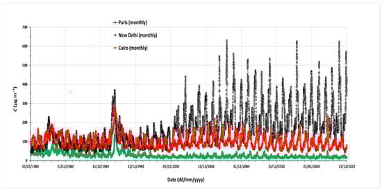
Figure 1. Reconstruction of the temporal evolution of the monthly averages of the PM10 concentrations in New Delhi (black points), Cairo (red points), and Paris (green points) between 1980 and 2024.

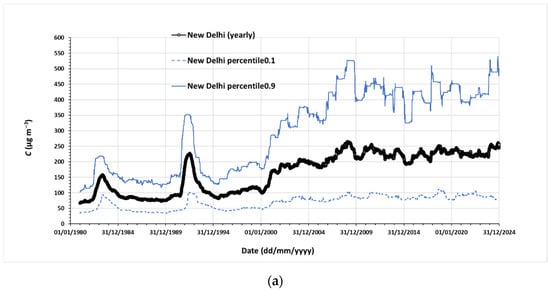
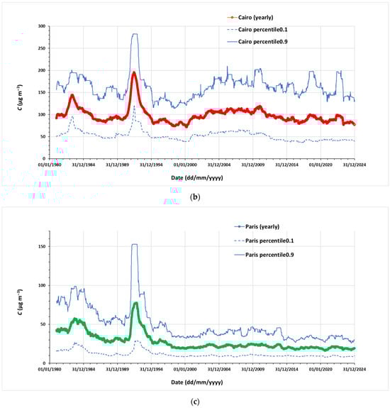
Figure 2. Same as Figure 1, but after application of a rolling average over durations of 1 year. The time stamp is at the end of the year, and (a) corresponds to New Delhi, (b) to Cairo, and (c) to Paris. The discontinuous and continuous blue lines represent the evolution of the 10th and 90th percentiles, respectively, of the statistical distributions of the daily values of the previous year.

This makes of them 2 of the 3 most violent eruptions of the northern hemisphere between 1980 and 2024 (the third one was Mount St. Helens whose eruption lasted from 1980 to 1986). Their plumes reached the stratosphere and increased the AOD for several months. Therefore, these cases do not meet the conditions of applications of Equation (3). The increase in the AOD is not correlated with a parallel increase in the PM10 concentration at the surface, and the latter is overestimated by the empirical method. Interestingly, the major eruptions of the Puyehue-Cordón Caulle (Chile; VEI = 5) in 2011 and of the Hunga Ha’apai (Tonga Islands; VEI = 5) in 2021 do not leave any visible trace on the plots of Figure 2. This can be explained by the fact that although the volcanic aerosols injected into the stratosphere did travel around the world, they did so at latitudes too south to have an impact on the retrievals of the surface concentrations in megacities of the northern hemisphere.

3.3. Discussion

For the derivation of the surface concentration from remote sensing observations, the AOD/C ratio is crucial. The difficulty is that its mean is not only different at the three reference sites of this study, but also quite variable (Table 6). The value at Paris-Les Halles (6.76·10⁻³ m³ µg⁻¹) is larger than that of New Delhi (3.01·10⁻³ m³ µg⁻¹) and Cairo (3.55·10⁻³ m³ µg⁻¹). This could be explained either by the fact that the concentration tends to be significantly larger close to the surface than in the rest of the PBL (larger mean value of k in Equation (3)), but also be due to a finer aerosol in Paris as suggested by the larger mean AE (1.26 in Paris vs. 0.91 in New Delhi and 1.08 in Cairo). The latter explanation would also be consistent with the more frequent presence of coarse dust particles in Egypt [50,52] and India [53,54] than in France.

Table 6. Mean and relative standard deviations (rSD, in %) of AOD/C, AE, PW, and H in the three megacities of this study. The rSD of the correction attributable to each input of Equation (3) is also reported. The values of the coefficients (C1, C2, and C3) yielded by the adjustment of Equation (3) to the concentration measurements performed at the experimental sites are also reported.

	Exp. 1	Paris	New Delhi	Cairo
AOD/C	Mean (m3 µg−1)	6.76 × 10−3	3.01 × 10−3	3.55 × 10−3
	rSD	62%	73%	35%
C1		−0.09	0.22	0.10
C2 (mm−1)		0.019	0.040	0.007
C3 (m−1)		6.22 × 10−4	3.42 × 10−4	9.18 × 10−5
AE	mean	1.26	0.91	1.08
	rSD	34%	42%	34%
	Correction_AE_rSD	3.9%	8.4%	3.7%
PW	Mean (mm)	15.8	20.8	16.3
	rSD	43%	62%	31%
	Correction_PW_rSD	12.9%	50.9%	14.0%
H	Mean (m)	610	576	726
	rSD	42%	49%	29%
	Correction_H_rSD	15.9%	9.6%	1.9%

In Equation (3), the variability of AOD/C at each site is assumed to be the result of the variability of AE, PW, and H, and a corrective factor of the form (1 + C_x ∗ (X − X_mean)) is associated with each of these variables. By definition, the mean of these factors is 1 after application of the LSR adjusting Equation (2) to the measurements. However, their relative standard deviations (Correction_X_rSD, in %) are more interesting: they quantify the variability of the corrections due individually to AE, PW, and H. For instance, the analysis of the results of Experiment 1, which was used because it provided the best results, shows that the variability of the correction linked with AE is more limited in Paris (3.9%) and Cairo (3.7%) than in New Delhi (8.4%). The difference is even more pronounced for PW: in New Delhi, if it were the sole variable of influence, PW would explain 50.9% of the variability of the AOD/C ratio. This is between 3 and 4 times more than in Paris or Cairo (12.9 and 14%, respectively). This predominant influence of PW in New Delhi can be explained by the large mean atmospheric humidity (20.8 mm, vs. 15.8 and 16.3 mm for Paris and Cairo), its marked variability (62%, vs. 43 and 31%), and also by a more hydrophilic nature of the aerosols indicated by a C2 (0.040 mm⁻¹) in the Indian capital that is about two to six times larger than in Paris and Cairo (0.019 and 0.007 mm⁻¹, respectively).

Finally, the influence of H is more pronounced in Paris (15.9%) and New Delhi (9.6%) than in Cairo (1.9%). In the latter megacity, clouds are rare in all seasons, and the temporal variability of the boundary layer height (29%) is less than in Paris (42%) where H drops dramatically during the winter months, and also less than in New Delhi (49%) where H is lower during the cloudy summer Monsoon months.

Despite these inter-site differences in aerosol characteristics (AE, affinity for water vapor) and climate (PW and H) conditions, the empirical method always provides the best results when the AERONET AOD, AE, and PW products are used as inputs. In the retrieval of C, AOD is obviously the most important variable. PW and AE are second-order ones, in the sense that they are only used to refine the value of the AOD/C ratio (via Equation (2)). This primary role of the AOD is confirmed by the comparison of the metrics of experiments 2, 3, and 4 with those of Experiment 1 (Table 7). At the three sites, replacing the AERONET AOD by that of MODIS, CAMS, or MERRA-2 leads to a systematic degradation of R, RMSE, and rMAE. This degradation is the largest at the daily temporal resolution, but the results improve at the weekly and monthly resolutions. This indicates that the satellite observations or the reanalyses products fail to reproduce the day-to-day variability of the AOD as measured by the AERONET sunphotometers, but that they better capture the variability at lower temporal resolutions, which enhances the performance of the empirical model. This is particularly true for Experiment 7 in Paris and New Delhi for which using the MERRA-2 AOD as a substitute for the AERONET one does not change the quality of the results. In Cairo, the results are not as good as in Paris or New Delhi, but they are also better when using the MERRA-2 AOD rather than the MODIS or CAMS ones.

Table 7. Evolution of the performance of the empirical model when replacing the original AERONET AOD, PW, and AE of Experiment 1 by (successively) MODIS, CAMS, and MERRA-2 products. At each site, the results are presented at the daily (1D), weekly (7D), and monthly (30D) temporal resolutions.

			Influence of AOD			Influence of PW			Influence of AE
Experiment		1	5	6	7	8	9	10	11	12	13
Paris
R	1D	0.74	0.50	0.61	0.69	0.73	0.74	0.71	0.73	0.74	0.71
RMSE (µg·m−3)	1D	8.4	13.0	10.7	8.6	8.6	8.5	8.9	8.7	8.4	8.9
rMAE (%)	1D	29	43	36	28	30	30	33	29	29	33
R	7D	0.82	0.58	0.73	0.80	0.81	0.82	0.79	0.78	0.82	0.78
RMSE (µg·m−3)	7D	5.0	9.3	6.7	5.1	5.2	5.1	5.1	5.4	5.0	5.1
rMAE (%)	7D	19	29	24	19	19	19	20	18	18	20
R	30D	0.84	0.64	0.78	0.88	0.81	0.83	0.75	0.82	0.84	0.74
RMSE (µg·m−3)	30D	3.8	6.8	5.3	3.8	3.9	3.9	3.6	4.4	3.8	3.7
rMAE (%)	30D	15	24	21	16	15	15	15	17	15	15
New Delhi
Experiment		1	5	6	7	8	9	10	11	12	13
R	1D	0.78	0.71	0.64	0.66	0.74	0.80	0.76	0.81	0.79	0.79
RMSE (µg·m−3)	1D	93.1	106.4	110.9	106.9	98.7	85.4	97.8	91.4	86.4	89.9
rMAE (%)	1D	21	26	25	23	25	23	23	21	21	21
R	7D	0.85	0.80	0.76	0.81	0.85	0.89	0.85	0.90	0.87	0.87
RMSE (µg·m−3)	7D	57.7	64.6	68.8	60.6	54.3	45.9	62.3	51.4	49.1	54.7
rMAE (%)	7D	15	18	19	16	15	14	17	13	14	15
R	30D	0.95	0.95	0.91	0.95	0.96	0.98	0.94	0.98	0.98	0.96
RMSE (µg·m−3)	30D	36.7	34.4	43.1	32.7	28.3	18.8	42.4	29.7	23.4	34.5
rMAE (%)	30D	11	14	16	10	10	8	13	11	10	11
Cairo
Experiment		1	5	6	7	8	9	10	11	12	13
R	1D	0.78	0.53	0.54	0.63	0.60	0.61	0.78	0.58	0.62	0.78
RMSE (µg·m−3)	1D	40.3	66.3	61.9	42.0	61.7	60.3	34.0	59.9	59.6	33.9
rMAE (%)	1D	23	39	34	30	30	30	23	30	29	23
R	7D	0.83	0.65	0.61	0.69	0.66	0.66	0.82	0.58	0.68	0.81
RMSE (µg·m−3)	7D	23.4	39.1	38.8	29.9	38.5	38.4	22.7	39.1	37.3	23.0
rMAE (%)	7D	15	25	24	20	22	23	15	23	22	15
R	30D	0.84	0.73	0.61	0.68	0.73	0.71	0.81	0.66	0.73	0.80
RMSE (µg·m−3)	30D	17.4	30.0	30.1	22.6	29.1	29.1	16.9	29.0	28.3	17.3
rMAE (%)	30D	12	22	22	16	19	20	12	20	20	12

Even at the daily resolution, using the PW (experiments 8, 9, and 10) and AE (experiments 11, 12, and 13) products of MODIS, CAMS, or MERRA-2 instead of the AERONET ones does not make any significant difference in Paris or New Delhi. This suggests that all these products are of similar quality in the two megacities. Conversely, in Cairo, the results yielded by the empirical model with the MERRA-2 PW (experiment 12) and AE (experiment 13) are globally better than those obtained with the other inputs.

4. Summary and Conclusions

Pluriannual time series of surface mass concentration of particulate matter are essential to evaluate the efficiency of policies aiming to control air pollution in urban areas. When in situ measurements do not exist or have many gaps, which is the case in many megacities of the developing world, two types of methods can be used to estimate the missing concentrations: reanalyses in which observations are assimilated to constrain a chemistry/transport model, and empirical models deriving the surface concentration from remote sensing products. In both cases, the availability of satellite observations since ca. 1980 allows the reconstruction of uninterrupted time series spanning more than 4 decades. In this work, we evaluated the ability of two widely used reanalyses (CAMS and MERRA-2) and of a recently developed empirical method (S2023) to retrieve the PM10 surface concentration in Paris, Cairo, and New Delhi. These megacities were chosen because they are located in different climate zones, they are all facing air-quality issues though of different severity, and they have also passed more or less strict regulations to curb their pollution problem.

The empirical method was used in different configurations: its inputs (namely the aerosol optical depth, Angström Exponent, and the atmospheric columnar content in precipitable water) were either derived from AERONET or satellite (MODIS) observations, or provided by the CAMS and MERRA-2 reanalyses. The best results were obtained with the AERONET inputs, but at the weekly and monthly temporal resolutions, they were of equivalent quality with the MERRA-2 inputs. This allowed the reconstruction of the PM10 time series from 1980 to 2024 in the three megacities of this study. The limitation of the method is due to the major eruptions of the El Chichon (1982) and Pinatubo (1991) volcanoes whose plumes reached the stratosphere and increased the AOD for several months in the northern hemisphere. Then, one of the assumptions underlying the empirical method—namely that the aerosols are found within the Boundary Layer and not above it—is not met, and this leads to an overestimation of the surface concentration.

When not considering these two very specific periods, it could be shown that in the last 45 years, the average concentration has more than trebled in New Delhi, (from 70 to 250 µg·m⁻³), has been divided by two in Paris (from 40 to 20 µg·m⁻³), and remained stable (around 100 µg·m⁻³) in Cairo. These different evolutions reflect the efficiencies of the measures taken (or not) to improve air quality. The method could be easily adapted to any other megacity in which the surface measurements necessary (one year or more) to calibrate the model are available.

References

- Intergovernmental Panel on Climate Change (IPCC). Climate Change 2021: The Physical Science Basis; Intergovernmental Panel on Climate Change (IPCC): Geneva, Switzerland, 2021; Available online: https://www.ipcc.ch (accessed on 15 June 2025).
- World Health Organization. Air Pollution and Health; World Health Organization: Geneva, Switzerland, 2021; Available online: https://www.who.int (accessed on 15 June 2025).
- Brook, R.D.; Rajagopalan, S.; Pope, C.A., III.; Brook, J.R.; Bhatnagar, A.; Diez-Roux, A.V.; Holguin, F.; Hong, Y.; Luepker, R.V.; Mittleman, M.A.; et al. Particulate Matter Air Pollution and Cardiovascular Disease: An Update to the Scientific Statement from the American Heart Association. Circulation 2010, 121, 2331–2378. [Google Scholar] [CrossRef]
- Emberson, L.D.; Ashmore, M.R.; Murray, F.; Kuylenstierna, J.C.I.; Percy, K.E.; Izuta, T.; Zheng, Y.; Shimizu, H.; Sheu, B.H.; Liu, C.P.; et al. Impacts of Air Pollutants on Vegetation in Developing Countries. Water Air Soil Pollut. 2001, 130, 107–118. [Google Scholar] [CrossRef]
- U.S. Environmental Protection Agency (EPA). Effects of Acid Rain; U.S. Environmental Protection Agency (EPA): Washington, DC, USA, 2023. Available online: https://www.epa.gov (accessed on 15 June 2025).
- Lo, W.-C.; Hu, T.-H.; Hwang, J.-S. Lifetime Exposure to PM2.5 Air Pollution and Disability Adjusted Life Years Due to Cardiopulmonary Disease: A Modeling Study Based on Nationwide Longitudinal Data. Sci. Total Environ. 2023, 855, 158901. [Google Scholar] [CrossRef]
- Lelieveld, J.; Evans, J.S.; Fnais, M.; Giannadaki, D.; Pozzer, A. The Contribution of Outdoor Air Pollution Sources to Premature Mortality on a Global Scale. Nature 2015, 525, 367–371. [Google Scholar] [CrossRef]
- Sicard, P.; Agathokleous, E.; Anenberg, S.C.; De Marco, A.; Paoletti, E.; Calatayud, V. Trends in Urban Air Pollution over the Last Two Decades: A Global Perspective. Science of The Total Environment 2023, 858 Pt 2, 160064. [Google Scholar] [CrossRef] [PubMed]
- European Commission. Directive (EU) 2024/2881 of the European Parliament and of the Council of 23 October 2024 on ambient air quality and cleaner air for Europe (recast). Off. J. Eur. Union 2024. Available online: https://eur-lex.europa.eu/eli/dir/2024/2881/oj/eng (accessed on 1 July 2025).
- European Environment Agency. Europe’s Air Quality Status 2024: Briefing; European Environment Agency: Luxembourg, 2024; Available online: https://www.eea.europa.eu/publications/europes-air-quality-status-2024 (accessed on 1 July 2025).
- U.S. Environmental Protection Agency. Final Reconsideration of the National Ambient Air Quality Standards for Particulate Matter (PM NAAQS); EPA: Washington, DC, USA, 2024. Available online: https://www.epa.gov/pm-pollution/final-reconsideration-national-ambient-air-quality-standards-particulate-matter-pm (accessed on 1 July 2025).
- Shi, Y.; Matsunaga, T.; Yamaguchi, Y.; Zhao, A.; Li, Z.; Gu, X. Long-Term Trends and Spatial Patterns of PM2.5-Induced Premature Mortality in Major Urban Areas of China. Sci. Total Environ. 2019, 631–632, 1504–1514. [Google Scholar] [CrossRef]
- European Environment Agency. Harm to Human Health from Air Pollution in Europe; EEA Report No 24/2023; European Environment Agency: Luxembourg, 2023; Available online: https://www.eea.europa.eu/publications/harm-to-human-health-from-air-pollution (accessed on 1 July 2025).
- Cooper, M.J.; Martin, R.V.; Hammer, M.S.; van Donkelaar, A.; Lyapustin, A.; Sayer, A.M.; Hsu, N.C.; Krotkov, N.A.; Brook, J.R.; Mallick, A.; et al. Global Fine-Scale Changes in Ambient NO2 during COVID-19 Lockdowns. Nature 2022, 601, 380–387. [Google Scholar] [CrossRef] [PubMed]
- Rodríguez-Urrego, D.; Rodríguez-Urrego, L. Air Quality during the COVID-19: PM2.5 Analysis in the 50 Most Polluted Capital Cities in the World. Environ. Pollut. 2020, 266, 115042. [Google Scholar] [CrossRef]
- Putaud, J.-P.; Pisoni, E.; Mangold, A.; Hueglin, C.; Sciare, J.; Pikridas, M.; Savvides, C.; Ondracek, J.; Mbengue, S.; Wiedensohler, A.; et al. Impact of 2020 COVID-19 Lockdowns on Particulate Air Pollution across Europe. Atmos. Chem. Phys. 2023, 23, 10145–10161. [Google Scholar] [CrossRef]
- Viatte, C.; Petit, J.-E.; Yamanouchi, S.; Van Damme, M.; Doucerain, C.; Germain-Piaulenne, E.; Gros, V.; Favez, O.; Clarisse, L.; Coheur, P.-F.; et al. Ammonia and PM2.5 Air Pollution in Paris during the 2020 COVID-19 Lockdown. Atmosphere 2021, 12, 160. [Google Scholar] [CrossRef]
- Sicard, P.; De Marco, A.; Agathokleous, E.; Feng, Z.; Xu, X.; Paoletti, E.; Diéguez Rodríguez, J.J.; Calatayud, V. Amplified ozone pollution in cities during the COVID-19 lockdown. Sci. Total Environ. 2020, 735, 139542. [Google Scholar] [CrossRef] [PubMed]
- Cuesta, J.; Costantino, L.; Beekmann, M.; Siour, G.; Menut, L.; Bessagnet, B.; Landi, T.C.; Dufour, G.; Eremenko, M. Ozone pollution during the COVID-19 lockdown in the spring of 2020 over Europe, analysed from satellite observations, in situ measurements, and models. Atmos. Chem. Phys. 2022, 22, 4471–4489. [Google Scholar] [CrossRef]
- Liu, Y.; Wang, T.; Stavrakou, T.; Elguindi, N.; Doumbia, T.; Granier, C.; Bouarar, I.; Gaubert, B.; Brasseur, G.P. Diverse Response of Surface Ozone to COVID-19 Lockdown in China. Sci. Total Environ. 2021, 789, 147739. [Google Scholar] [CrossRef]
- Mostafa, A.N.; Alfaro, S.; Cuesta, J.; Hassan, I.A.; Abdel Wahab, M.M. Surface Ozone Variability in Two Contrasting Megacities, Cairo and Paris, and Its Observation from Satellites. Atmosphere 2025, 16, 475. [Google Scholar] [CrossRef]
- Wang, J.; Christopher, S.A. Intercomparison between Satellite-Derived Aerosol Optical Thickness and PM2.5 Mass: Implications for Air Quality Studies. Geophys. Res. Lett. 2003, 30, 2095. [Google Scholar] [CrossRef]
- Gupta, P.; Christopher, S.A. Particulate Matter Air Quality Assessment Using Integrated Surface, Satellite, and Meteorological Products: A Neural Network Approach. J. Geophys. Res. Atmos. 2009, 114, D20205. [Google Scholar] [CrossRef]
- Shin, M.; Kang, Y.; Park, S.; Im, J.; Yoo, C.; Quackenbush, L.J. Estimating Ground-Level Particulate Matter Concentrations Using Satellite-Based Data: A Review. GIScience Remote Sens. 2020, 57, 174–189. [Google Scholar] [CrossRef]
- Inness, A.; Ades, M.; Agustí-Panareda, A.; Barré, J.; Benedictow, A.; Blechschmidt, A.M.; Dominguez, J.J.; Engelen, R.; Eskes, H.; Flemming, J.; et al. The CAMS Reanalysis of Atmospheric Composition. Atmos. Chem. Phys. 2019, 19, 3515–3556. [Google Scholar] [CrossRef]
- Li, Y.; Dhomse, S.S.; Chipperfield, M.P.; Feng, W.; Chrysanthou, A.; Xia, Y.; Guo, D. Effects of Reanalysis Forcing Fields on Ozone Trends and Age of Air from a Chemical Transport Model. Atmos. Chem. Phys. 2022, 22, 10635–10656. [Google Scholar] [CrossRef]
- Molod, A.; Takacs, L.; Suarez, M.; Bacmeister, J. Development of the GEOS-5 Atmospheric General Circulation Model: Evolution from MERRA to MERRA-2. Geosci. Model Dev. 2015, 8, 1339–1356. [Google Scholar] [CrossRef]
- Li, X.; Wang, Y.; Hu, X.; Zhang, W. Estimating Ground-Level PM2.5 Using AOD Retrievals from Satellite Observations and WRF-Chem Simulations. Atmos. Res. 2018, 214, 47–58. [Google Scholar] [CrossRef]
- Hu, X.; Belle, J.H.; Meng, X.; Wildani, A.; Waller, L.A.; Strickland, M.J.; Liu, Y. Estimating PM2.5 Concentrations in the Conterminous United States Using the Random Forest Approach. Environ. Sci. Technol. 2017, 51, 6936–6944. [Google Scholar] [CrossRef] [PubMed]
- Brokamp, C.; Jandarov, R.; Hossain, M.; Ryan, P. Predicting Daily Urban Fine Particulate Matter Concentrations Using a Random Forest Model. Environ. Sci. Technol. 2018, 52, 4173–4179. [Google Scholar] [CrossRef] [PubMed]
- Gupta, P.; Christopher, S.A. Particulate Matter Air Quality Assessment Using Integrated Surface, Satellite, and Meteorological Products: Multiple Regression Approach. J. Geophys. Res. Atmos. 2009, 114, D14205. [Google Scholar] [CrossRef]
- Zou, B.; Liu, L.; Huang, L.; Li, Z.; Li, D. Satellite-Based PM10 Estimation and Its Comparison with Reanalysis Datasets. Atmos. Pollut. Res. 2016, 7, 512–521. [Google Scholar]
- Tian, M.; Chen, Y. Correction of Vertical AOD Profiles for PM2.5 Estimation Using Planetary Boundary Layer Height and Relative Humidity. Atmos. Environ. 2010, 44, 905–910. [Google Scholar] [CrossRef]
- He, Q.; Huang, B. Satellite-Based Mapping of Daily High-Resolution Ground PM2.5 in China via Space-Time Regression Modeling. Remote Sens. Environ. 2018, 206, 72–83. [Google Scholar] [CrossRef]
- Said, S.; Salah, Z.; Abdel Wahab, M.M.; Alfaro, S.C. Retrieving PM10 Surface Concentration from AERONET Aerosol Optical Depth: The Cairo and Delhi Megacities Case Studies. J. Indian Soc. Remote Sens. 2023, 51, 1797–1807. [Google Scholar] [CrossRef]
- Holben, B.N.; Eck, T.F.; Slutsker, I.; Tanré, D.; Buis, J.P.; Setzer, A.; Vermote, E.; Reagan, J.A.; Kaufman, Y.J.; Nakajima, T.; et al. AERONET—A Federated Instrument Network and Data Archive for Aerosol Characterization. Remote Sens. Environ. 1998, 66, 1–16. [Google Scholar] [CrossRef]
- Giles, D.M.; Sinyuk, A.; Sorokin, M.G.; Schafer, J.S.; Smirnov, A.; Slutsker, I.; Eck, T.F.; Holben, B.N.; Lewis, J.R.; Campbell, J.R.; et al. Advancements in the Aerosol Robotic Network (AERONET) Version 3 Database—Automated Near-Real-Time Quality Control Algorithm with Improved Cloud Screening for Sun Photometer Aerosol Optical Depth (AOD) Measurements. Atmos. Meas. Tech. 2019, 12, 169–209. [Google Scholar] [CrossRef]
- Sinyuk, A.; Holben, B.N.; Eck, T.F.; Giles, D.M.; Slutsker, I.; Korkin, S.; Schafer, J.S.; Smirnov, A.; Sorokin, M.; Lyapustin, A. The AERONET Version 3 Aerosol Retrieval Algorithm, Associated Uncertainties and Comparisons to Version 2. Atmos. Meas. Tech. 2020, 13, 3375–3411. [Google Scholar] [CrossRef]
- Ångström, A. The Parameters of Atmospheric Turbidity. Tellus 1964, 16, 64–75. [Google Scholar] [CrossRef]
- Lei, L.; Sun, Y.; Ouyang, B.; Qiu, Y.; Xie, C.; Tang, G.; Zhou, W.; He, Y.; Wang, Q.; Cheng, X.; et al. Vertical Distributions of Primary and Secondary Aerosols in Urban Boundary Layer: Insights into Sources, Chemistry, and Interaction with Meteorology. Environ. Sci. Technol. 2021, 55, 4542–4552. [Google Scholar] [CrossRef]
- Mostafa, A.N.; Zakey, A.S.; Monem, A.S.; Abdel Wahab, M.M.A. Analysis of the Surface Air Quality Measurements in the Greater Cairo (Egypt) Metropolitan. Glob. J. Adv. Res. 2018, 5, 207–214. [Google Scholar]
- Hyvärinen, A.-P.; Lihavainen, H.; Komppula, M.; Panwar, T.S.; Sharma, V.P.; Hooda, R.K.; Viisanen, Y. Aerosol measurements at the Gual Pahari EUCAARI station: Preliminary results from in-situ measurements. Atmos. Chem. Phys. 2010, 10, 7241–7252. [Google Scholar] [CrossRef]
- Buchard, V.; Randles, C.A.; Da Silva, A.M.; Darmenov, A.; Colarco, P.R.; Govindaraju, R.; Ferrare, R.; Hair, J.; Beyersdorf, A.J.; Ziemba, L.D.; et al. The MERRA-2 Aerosol Reanalysis, 1980 Onward. Part II: Evaluation and Case Studies. J. Clim. 2017, 30, 6851–6872. [Google Scholar] [CrossRef]
- Randles, C.A.; Da Silva, A.M.; Buchard, V.; Colarco, P.R.; Darmenov, A.; Govindaraju, R.; Smirnov, A.; Holben, B.; Ferrare, R.; Hair, J.; et al. The MERRA-2 Aerosol Reanalysis, 1980 Onward. Part I: System Description and Data Assimilation Evaluation. J. Clim. 2017, 30, 6823–6850. [Google Scholar] [CrossRef]
- Gueymard, C.A.; Yang, D. Worldwide validation of CAMS and MERRA-2 reanalysis aerosol optical depth products using 15 years of AERONET observations. Atmos. Environ. 2020, 225, 117216. [Google Scholar] [CrossRef]
- Schober, P.; Boer, C.; Schwarte, L.A. Correlation Coefficients: Appropriate Use and Interpretation. Anesth. Analg. 2018, 126, 1763–1768. [Google Scholar] [CrossRef]
- Reich, N.G.; Lessler, J.; Sakrejda, K.; Lauer, S.A.; Iamsirithaworn, S.; Cummings, D.A.T. Case Study in Evaluating Time Series Prediction Models Using the Thailand Dengue Surveillance System. Epidemics 2016, 17, 33–43. [Google Scholar] [CrossRef]
- World Health Organization (WHO). WHO Global Air Quality Guidelines: Particulate Matter (PM2.5 and PM10), Ozone, Nitrogen Dioxide, Sulfur Dioxide and Carbon Monoxide; World Health Organization: Geneva, Switzerland, 2021; Available online: https://www.who.int/publications/i/item/9789240034228 (accessed on 19 September 2025).
- de Bont, J.; Krishna, B.; Stafoggia, M.; Banerjee, T.; Dholakia, H.; Garg, A.; Ingole, V.; Jaganathan, S.; Kloog, I.; Lane, K.; et al. Ambient Air Pollution and Daily Mortality in Ten Cities of India: A Causal Modelling Study. Lancet Planet. Health 2024, 8, e433–e440. [Google Scholar] [CrossRef]
- El-Metwally, M.; Alfaro, S.C.; Abdel Wahab, M.; Chatenet, B. Aerosol Characteristics over Urban Cairo: Seasonal Variations as Retrieved from Sun Photometer Measurements. J. Geophys. Res. Atmos. 2008, 113, D14219. [Google Scholar] [CrossRef]
- Global Volcanism Program. Volcanoes of the World; v. 5.2.8; Venzke, E., Ed.; Smithsonian Institution: Washington, DC, USA, 2024. [Google Scholar] [CrossRef]
- Boraiy, M.; El-Metwally, M.; Wheida, A.; El-Nazer, M.; Hassan, S.K.; El-Sanabary, F.F.; Alfaro, S.C.; Abdelwahab, M.; Borbon, A. Statistical analysis of the variability of reactive trace gases (SO2, NO2 and ozone) in Greater Cairo during dust storm events. J. Atmos. Chem. 2023, 80, 227–250. [Google Scholar] [CrossRef]
- Leon, J.-F.; Chazette, P.; Dulac, F.; Pelon, J.; Flamant, C.; Ramdriamiarisoa, H.; Cautenet, G. Large-scale advection of continental aerosols during INDOEX. J. Geophys. Res. Atmos. 2001, 106, 28427–28439. [Google Scholar] [CrossRef]
- Alfaro, S.C.; Gaudichet, A.; Rajot, J.L.; Gomes, L.; Maillé, M.; Cachier, H. Variability of aerosol size-resolved composition at an Indian coastal site during the Indian Ocean Experiment (INDOEX) Intensive Field Phase. J. Geophys. Res. Atmos. 2003, 108, 8641. [Google Scholar] [CrossRef]
Disclaimer/Publisher’s Note: The statements, opinions and data contained in all publications are solely those of the individual author(s) and contributor(s) and not of MDPI and/or the editor(s). MDPI and/or the editor(s) disclaim responsibility for any injury to people or property resulting from any ideas, methods, instructions or products referred to in the content. |
© 2025 by the authors. Licensee MDPI, Basel, Switzerland. This article is an open access article distributed under the terms and conditions of the Creative Commons Attribution (CC BY) license (https://creativecommons.org/licenses/by/4.0/).