Article

Near-Surface Temperature Prediction Based on Dual-Attention-BiLSTM

Department of Mathematical and Physics, Shijiazhuang Tiedao University, 17 Northeast Second Inner Ring, Shijiazhuang 050043, China
*
Author to whom correspondence should be addressed.
Atmosphere 2025, 16(10), 1175; https://doi.org/10.3390/atmos16101175
Submission received: 22 August 2025 / Revised: 4 October 2025 / Accepted: 6 October 2025 / Published: 10 October 2025
(This article belongs to the Section Meteorology)

Abstract

Current temperature prediction methods often focus on time-series information while neglecting the contributions of different meteorological factors and the context of varying time steps. Accordingly, this study developed a Dual-Attention-BiLSTM (a bidirectional long short-term memory network with dual attention mechanisms) network model, which integrates a bidirectional long short-term memory (BiLSTM) network model with random forest-based feature selection and two self-designed attention mechanisms. A sensitivity analysis was conducted to evaluate the influence of the attention mechanisms. This study focuses on Shijiazhuang City, China, which has a temperate continental monsoon climate with significant seasonal and daily variations. The data were sourced from ERA5-Land, comprising hourly near-surface temperature and related meteorological variables for the year of 2022. The results indicate that integrating the two attention mechanisms significantly improves the model’s prediction performance compared to using BiLSTM alone. The mean absolute error between simulation results ranges from 0.80 °C to 1.08 °C, with a reduction of 0.17 °C to 0.39 °C, and the root mean square error ranges from 1.17 °C to 1.37 °C, with a reduction of 0.12 °C to 0.22 °C.

1. Introduction

Changes in the Earth’s ozone layer and frequent human activities have led to global warming, rising sea levels, and an increase in extreme weather events [1]. In recent years, some regions of China have experienced significant warming trends, especially in Northern and Eastern China, which have experienced rising temperatures, droughts, and frequent extreme weather events [2]. China is located on the eastern side of the Eurasian continent, to the west of the northwest Pacific, and is affected by monsoon climates year-round [3]. The variability in the monsoon climates directly influences the temporal and spatial distributions of the surface temperature, which in turn affect the accuracy of temperature predictions [4]. Accurate temperature forecasting in localized regions is crucial for reducing secondary disasters caused by abnormal temperatures, minimizing agricultural and industrial losses, and ensuring the safety of people’s lives and property [5].
Researchers have typically relied on numerical models for temperature forecasting [6,7]. In recent years, machine learning, originating from artificial neural networks (ANNs), has become increasingly popular. By extracting data and mimicking brain functions, machine learning algorithms can interpret data features and model relationships to predict physical processes [8,9]. ANN models, including long short-term memory (LSTM) networks and convolutional neural networks (CNNs), have yielded promising results in temperature prediction research [10,11,12,13]. Studies abroad have also demonstrated that artificial neural networks perform well in temperature forecasting by effectively capturing the nonlinear characteristics of temperature data, thereby improving the prediction accuracy [14]. However, single neural network models still have limitations, especially in their homogeneous processing of input meteorological features, which overlooks the different impacts of various meteorological factors on temperature predictions. As a result, researchers are exploring the integration of other machine learning techniques to further enhance the prediction accuracy and stability [15,16,17]. The random forest (RF) model, which measures the importance of feature variables, can identify factors most strongly correlated with temperature and eliminate noise interference from raw meteorological data [18]. Attention mechanisms, a novel deep learning technology, have been widely applied in fields such as natural language processing, image recognition, and data prediction. These mechanisms focus the model on relevant information by assigning different weights to variables and time steps. Applying attention mechanisms to temperature prediction could improve the model’s ability to capture spatial and temporal temperature variations [19].
In this study, we used the fifth generation European Centre for Medium-Range Weather Forecasts (ECMWF) atmospheric reanalysis of the global climate (ERA5-land) reanalysis data for Shijiazhuang in 2022 and employed the random forest model for feature weight extraction. The attention mechanism considers the different impacts of meteorological features on temperature changes. A bidirectional LSTM (BiLSTM) temperature prediction model that incorporates the random forest model and attention mechanisms was developed to forecast near-surface temperatures for the next 12, 24, 36, and 48 h. The results of this study provide technical support for improving the accuracy of local near-surface temperature prediction.

2. Materials and Methods

2.1. Data

In this study, we focused on Shijiazhuang, Hebei Province, China (114.5° E, 38° N). This city is located on the eastern coast of the Eurasian continent (see Figure 1) and has a temperate continental monsoon climate. It experiences distinct seasonal changes, with significant temperature variations between seasons and between day and night. Additionally, the area is influenced by local and surrounding geographical features, leading to complex and distinct temporal and spatial temperature variations [20]. Given the representative nature of the temperature changes in this region, accurate short-term temperature forecasting is of practical significance for improving meteorological services, enhancing agricultural production, and improving the quality of life for residents.
The ERA5-land reanalysis data for Shijiazhuang in 2022 was used in this study. The data include hourly near-surface temperatures and five meteorological features strongly correlated with temperature: 10 m U-component wind, 10 m V-component wind, surface pressure, total precipitation, and near-surface dew point temperature. The data were obtained from the ERA5 reanalysis model’s land module, with a spatial resolution of 0.1° × 0.1° (original resolution of 9 km).

2.2. Attention Mechanism Design

The attention mechanism assigns different weights to various parts of the input sequence, allowing the model to focus on the most relevant information during long sequence processing [21]. However, traditional attention mechanisms only incorporate weight information in the hidden layer, and the model cannot analyze the contextual relationships at each time step. Additionally, traditional attention mechanisms focus on the importance of different time steps, treating features within the same time step as a whole and neglecting the varying contributions of different meteorological features. To address these issues, we propose two improved attention mechanisms: the key-value attention mechanism and feature attention mechanism.

2.2.1. Key-Value Attention Mechanism

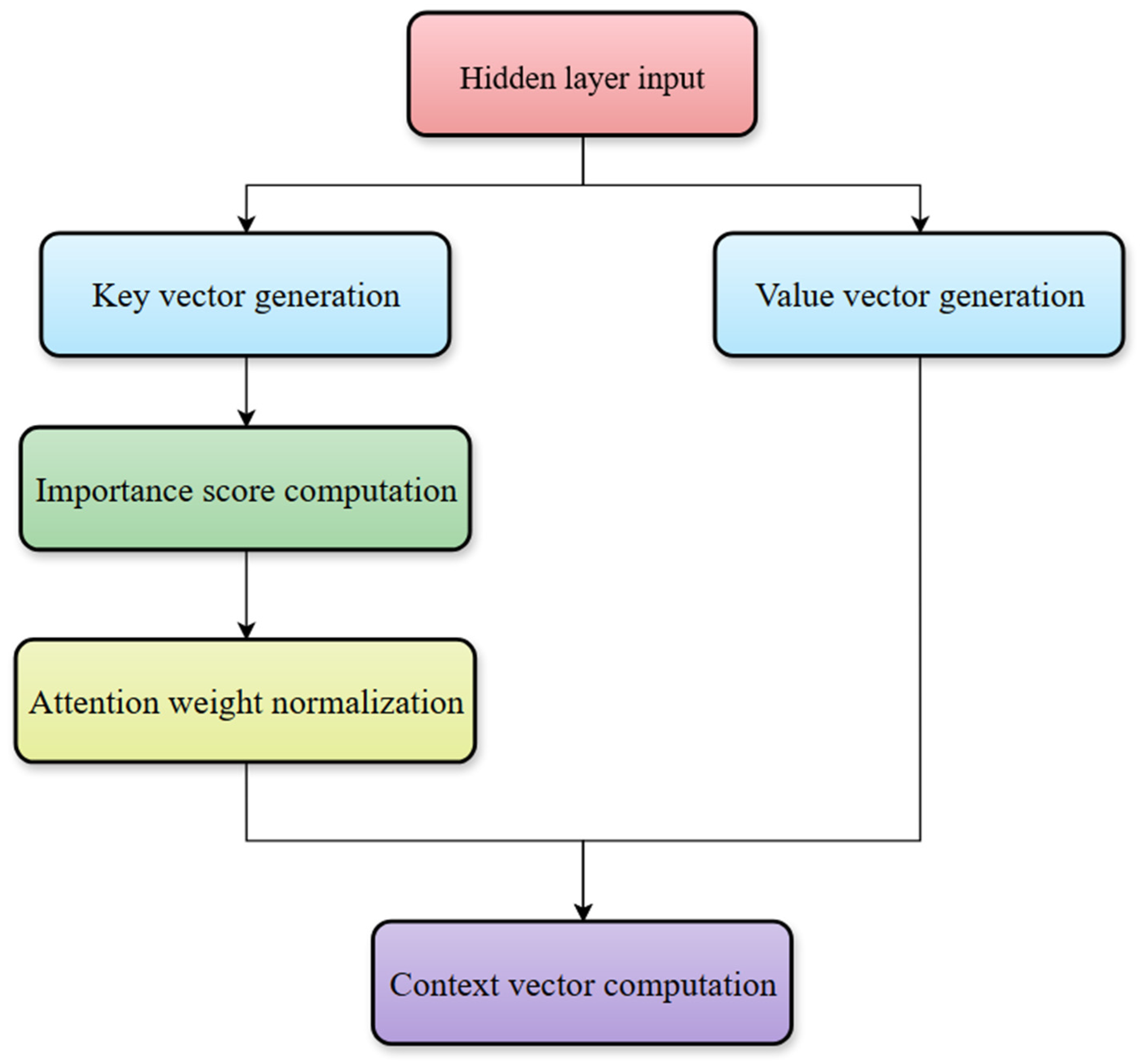
The key-value attention mechanism enhances the model’s learning ability by interpreting hidden layer information. The mechanism generates two independent mappings from the hidden layer: key and value vectors. The key vector measures the importance of each time step, while the value vector stores features closely related to temperature. The model calculates the dot product between the key vector and the model’s score vector, normalizes the score, and assigns attention weights. Higher weights indicate greater importance for the time step. The value vector stores rich semantic information about the time step, allowing the model to focus on important time steps and learn their feature information. Compared to traditional attention mechanisms, this mechanism enables the model to learn contextual information, improving its ability to capture sequential data features. The formulas for the Key-value Attention Mechanism are as follows:
K e y i ( 64 ) = tanh ( W k ( 64 × 64 ) h i ( 64 ) + b k ( 64 ) ) ,
V a l u e i ( 64 ) = W v ( 64 × 64 ) h i ( 64 ) + b v ( 64 ) ,
s c o r e i ( 1 ) = u ( 64 ) T K e y i ( 64 ) ,
α i ( 1 ) = exp ( s c o r e i ( 1 ) ) j = 1 n exp ( s c o r e j ( 1 ) ) ,
C o n t e x t ( 64 ) = i = 1 n α i ( 1 ) V a l u e i ( 64 ) ,
where K e y is the generate key vector; V a l u e is the generate value vector; s c o r e is the calculate importance score; α is the calculate attention weight; C o n t e x t is the generate context vector; h i is the hidden state produced by BiLSTM at the i-th time step; W k is the weight matrix for the key mapping; and b k is the bias for the key mapping. W v is the weight matrix for the value mapping; and b v is the bias for the value mapping. u is the score vector. n is the sequence length. W k , b k , W v , b v and u are initialized using the Glorot (Xavier) method.
The process of the key-value attention mechanism is illustrated in Figure 2.

2.2.2. Feature Attention Mechanism

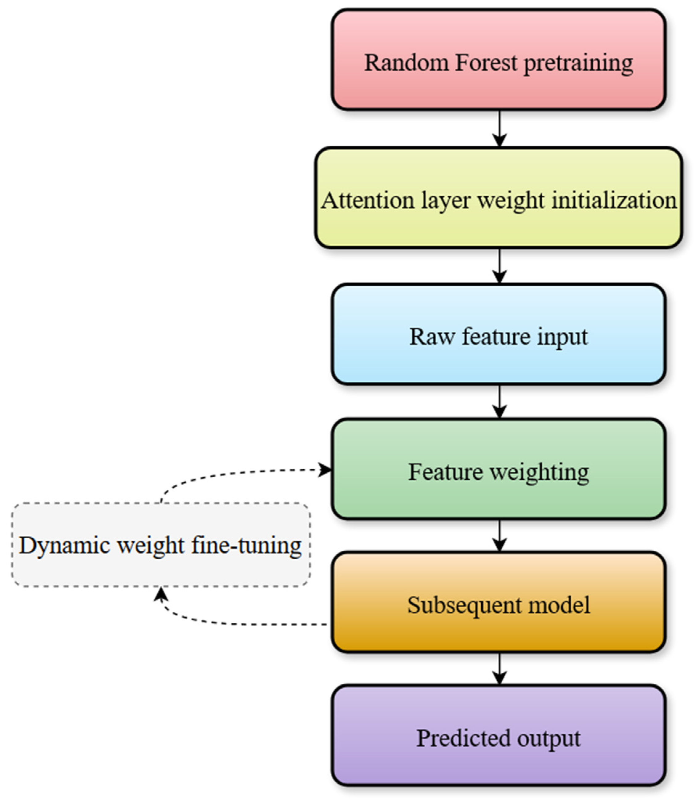
The feature attention mechanism enhances the model’s learning ability by considering the contributions of different features. The mechanism first uses the random forest model to compute the feature importance (RF_weights) and then initializes the attention layer’s weights using this information. Each training input is weighted by the attention layer before being passed to subsequent layers. This ensures that the model focuses on key features from the beginning of the training. In later training stages, the model dynamically adjusts the weights based on the training outcomes. Compared to traditional attention mechanisms, this approach enables the model to account for the contributions of each feature, reducing the impacts of low-contribution features and strengthening the learning of high-value features. The formulas for the Feature Attention Mechanism are as follows:
W ( 6 × 6 ) ( 0 ) = R F _ w e i g h t s ( 6 × 6 ) ,
x ( B × T × 6 ) = x ( B × T × 6 ) softmax ( x ( B × T × 6 ) W ( 6 × 6 ) + b ( 6 ) ) ,
W ( t + 1 ) = W ( t ) η w L ( y ^ , y ) ,
where W ( 0 ) is the initialize feature attention weight vector; x is the weighting applied to the model input; W ( t + 1 ) is the dynamically adjusted weights; R F _ w e i g h t s is the weight vector computed by the random forest algorithm; x is the model input; b is the bias for the feature attention mapping; B is the batch size of the model; and T is the number of time steps in each input sequence. η is the learning rate, and L ( y ^ , y ) is the loss function for the current training iteration of the model. b is initialized as a zero vector.
The process of the feature attention mechanism is illustrated in Figure 3.

2.2.3. BiLSTM Model with Attention Mechanisms

The LSTM is an improved version of the traditional recurrent neural network (RNN) and includes memory units and gating mechanisms. This model selectively retains or discards historical information, capturing long-term dependencies in sequential data [22]. However, the traditional LSTM can only process data in one direction, limiting its ability to use future information. The BiLSTM processes both forward and backward information flows, allowing for better capture of time dependencies and improving the prediction accuracy and stability [23].
The model developed in this study is a Dual-Attention-BiLSTM (BiLSTM with key-value and feature attention mechanisms). The model architecture includes an input layer, feature attention layer, BiLSTM layer, key-value attention layer, and output layer. The feature attention layer dynamically weights the different features, while the BiLSTM layer captures high-dimensional information through a three-layer BiLSTM network, with dropout layers added to reduce overfitting. The key-value attention layer uses key and value mappings to focus on important time steps and learn their features.

2.3. Random Forest Feature Extraction

The RF is an ensemble learning-based nonlinear predictive model. The main idea is to construct multiple decision trees through random sampling and feature selection, thereby reducing the model variance and improving the generalization ability [24]. In this study, we used the impurity splitting method to assess the importance of each feature. This method constructs decision trees using the classification and regression trees (CART) algorithm, which selects the optimal splitting feature and splitting point at each node to minimize impurity. The importance of each feature is measured by the cumulative reduction in the impurity across all the trees and all the nodes that use that feature for splitting.

2.4. Experiment Scheme Design

In deep learning model research, the combination of the model structure and methodology significantly influences the predictive performance of the model. To thoroughly evaluate the contribution of the method proposed in this study to the model accuracy, four different model schemes were designed for comparative analysis. The four model schemes are summarized in Table 1.
Scheme 1 uses only the BiLSTM model. Scheme 2 adds the feature attention mechanism on top of the BiLSTM. Scheme 3 adds the key-value attention mechanism to the BiLSTM. Scheme 4 is the complete Dual-Attention-BiLSTM model, which incorporates both attention mechanisms. All four schemes initialize the input data with feature weights calculated by the random forest model and perform normalization. Most existing studies set 48 h as the maximum prediction horizon [25], and since temperature is influenced by the day-night cycle, choosing multiples of 12 h (12/24/36/48 h) can cover both daytime and nighttime periods, thus meeting the need for differentiated predictions between day and night [26]. Therefore, this study sets the hourly temperature for the next 12, 24, 36, and 48 h as the prediction targets, with an input step size of 24 h.
In this study, we used a rolling window method for supervised learning, using historical data sequences to predict future hourly temperature changes. To prevent overfitting and enhance the training efficiency, we employed an early stopping mechanism [27]. This mechanism halts training when the loss function on the validation set does not decrease after 15 consecutive epochs, and the model parameters with the best performance on the validation set are saved. After multiple experiments, the model batch size was set to 32, and the maximum number of epochs was set to 150, aiming to balance the model performance and training efficiency.

2.5. Model Evaluation Metrics

Model evaluation metrics are crucial for assessing the prediction performance of the model. In this study, two statistical metrics, the mean absolute error (MAE) and root mean squared error (RMSE), were used. The MAE computes the average error between the predicted and observed values, reflecting the overall deviation in the predictions. The RMSE, by squaring the errors, averaging them, and then taking the square root, gives higher penalties to larger prediction errors, making it sensitive to temperature anomalies.

3. Results

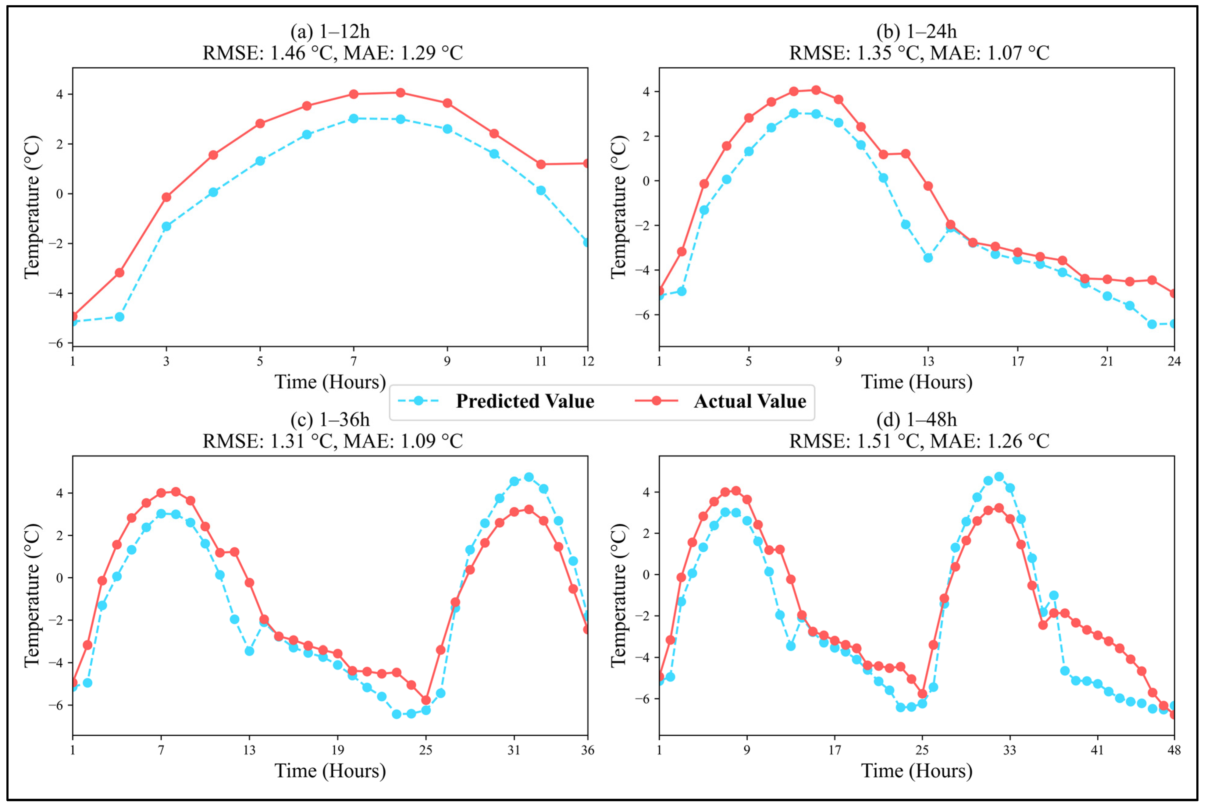
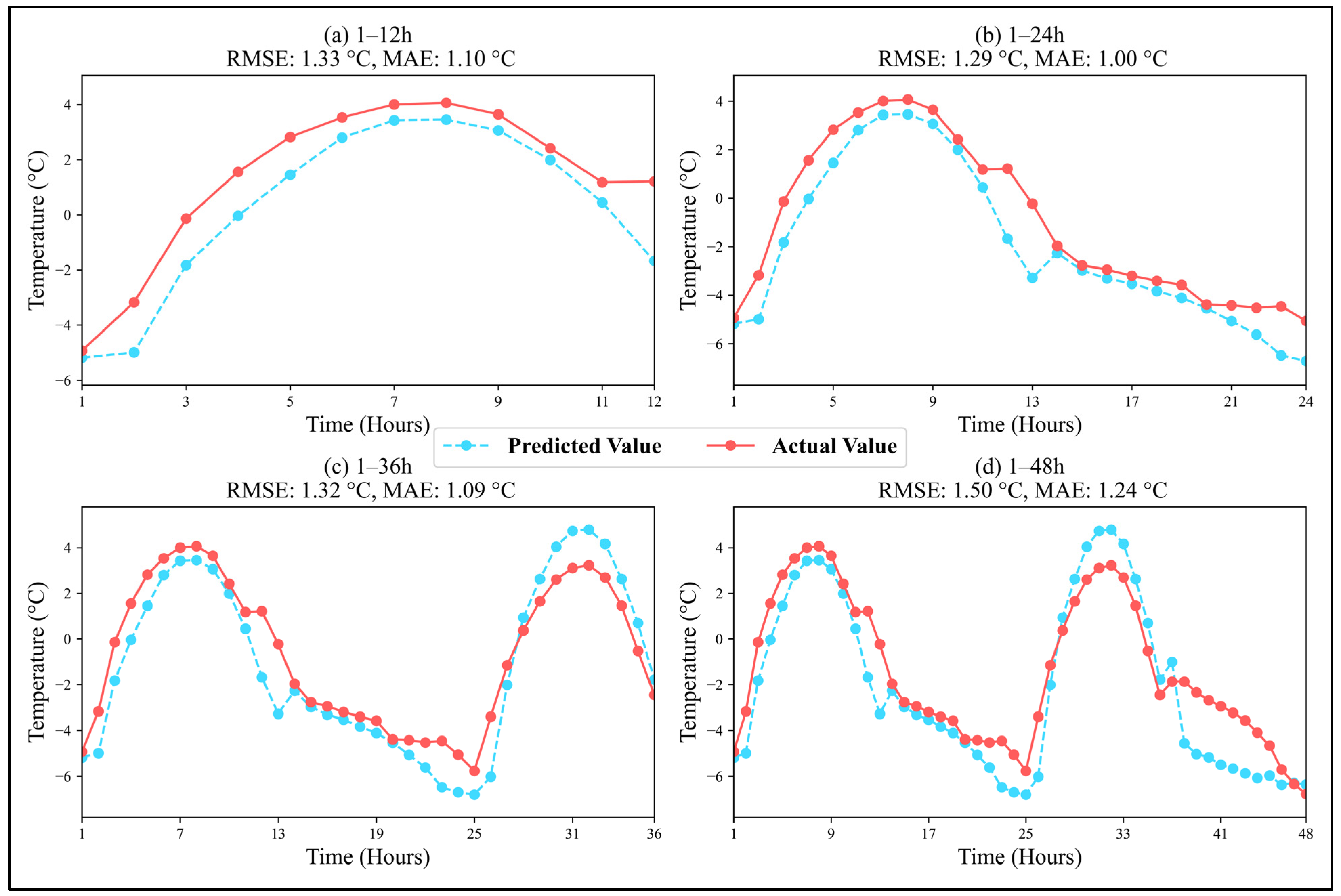
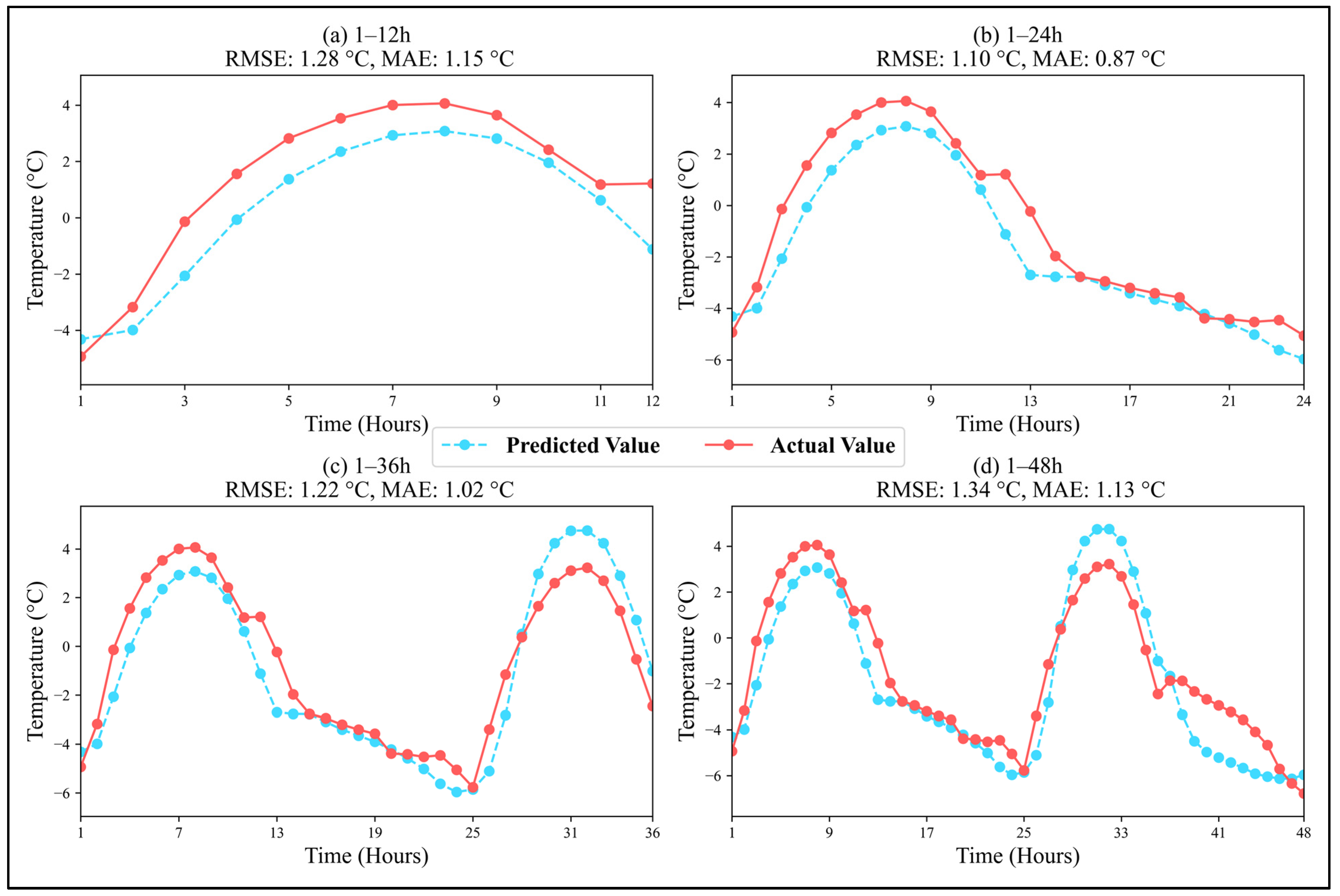
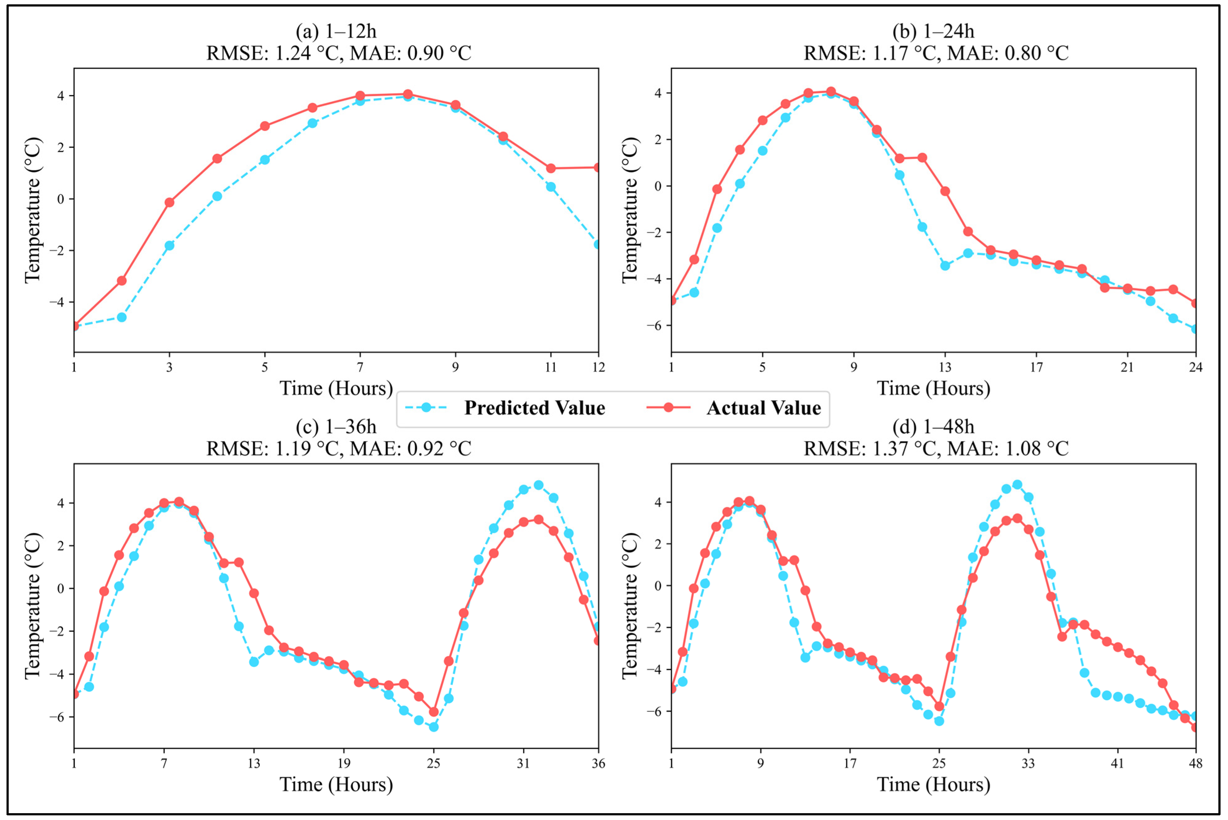
We trained and predicted the temperature using the four model schemes developed in this study. The results are shown in Figure 4, Figure 5, Figure 6 and Figure 7, showing that the models perform differently across the schemes. Scheme 1 (Figure 4) has the poorest performance, indicating that relying solely on the BiLSTM network fails to capture the complex characteristics of the temperature changes. Schemes 2 (Figure 5) and 3 (Figure 6) have better performances than Scheme 1, with the attention mechanisms playing a role in feature selection and dynamic weighting. The accuracy of the predictions for each time step is improved by 10–20%, suggesting that the introduction of either attention mechanism can enhance the model performance. Scheme 4 (Figure 7) has the best overall performance, with a prediction accuracy improvement of around 30% compared to Scheme 1, further proving that the inclusion of both attention mechanisms can significantly improve the prediction performance.
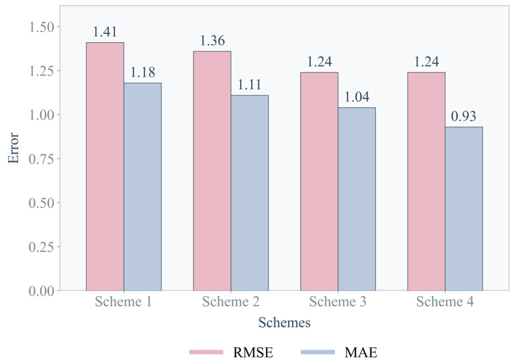
Finally, we calculated the average MAE and RMSE for each scheme at the four time intervals and plotted the prediction errors in Figure 8. As shown in the figure, the RMSE and MAE for Scheme 1 are 1.41 °C and 1.18 °C, respectively. For Scheme 2, the errors are 1.36 °C and 1.11 °C, representing a 3.5% reduction in RMSE and a 5.9% reduction in MAE compared to Scheme 1. For Scheme 3, the errors are 1.23 °C and 1.04 °C, showing a 12.8% decrease in RMSE and an 11.9% decrease in MAE compared to Scheme 1. For Scheme 4, the errors are 1.24 °C and 0.92 °C, with a 12.1% reduction in RMSE and a 22.0% reduction in MAE compared to Scheme 1. The results show that Scheme 1 has the largest error, while Schemes 2 and 3 have similar errors that are smaller than those of Scheme 1. Scheme 4 has the smallest errors. This further confirms that the dual attention mechanisms significantly enhance the overall accuracy of the model.

4. Discussion

4.1. Comparison of Three Models

The applicability of temperature prediction models is typically influenced by local climate characteristics and topography, with temperature fluctuations in inland areas often differing significantly from those in coastal or plain regions. However, different modeling methods and approaches can help explore more possibilities for inland temperature prediction. Therefore, models that perform excellently in other regions are still worth comparing and drawing insights from when applied to inland areas. Accordingly, we benchmarked the proposed Dual-Attention-BiLSTM model against the established BiLSTM-Kalman [28] and TD-LSTM [29] models for surface temperature prediction in Shijiazhuang City, Hebei Province.
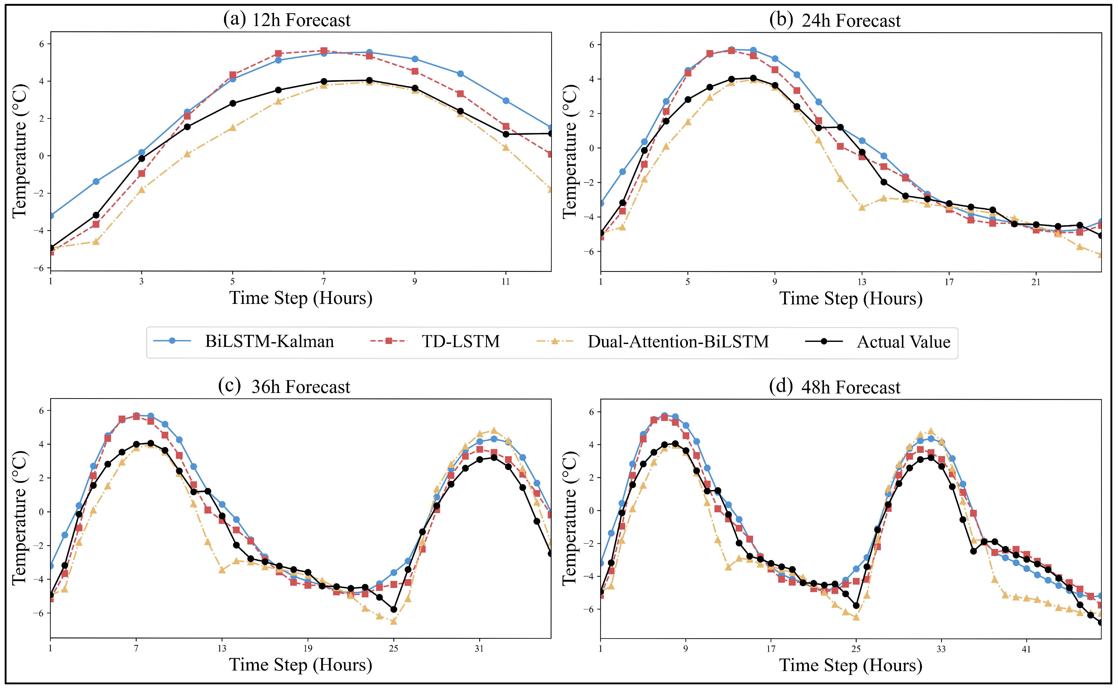
To verify the performance of the above two studies in inland temperature prediction, this research replicated the BiLSTM-Kalman framework and TD-LSTM model following the original approaches. The models were trained and tested using the dataset employed in this study. All training and prediction processes used the same dataset, with prediction targets being the temperatures for the next 12, 24, 36, and 48 h. To provide a clearer comparison of the results, this study presents the prediction errors of the Dual-Attention-BiLSTM, BiLSTM-Kalman, and TD-LSTM models in Table 2, and the prediction results are plotted in Figure 9.
From the error data in Table 2, the TD-LSTM model consistently performs the best across all prediction durations, maintaining low errors in both short-term and long-term predictions. While the Dual-Attention-BiLSTM model performs well in short-term predictions, its error significantly increases at 48 h, indicating poor stability in long-term predictions. The BiLSTM-Kalman model, on the other hand, exhibits substantial fluctuations in errors, especially at 12 h, indicating generally lower prediction accuracy. Therefore, the TD-LSTM model performs the best, followed by the Dual-Attention-BiLSTM model, and the BiLSTM-Kalman model performs the worst.
From the prediction results in Figure 9, it can be seen that more than half of the predictions made by the TD-LSTM and BiLSTM-Kalman models exceed the observed values, especially the predicted values at the peak temperature are nearly 2 °C higher than the observed values. In the operational forecasting of near surface temperatures, if the predicted values are higher than the actual temperature, it will be difficult to provide effective meteorological freezing disaster warnings for social production due to insufficient estimation of low temperatures, resulting in economic losses in agriculture and industry. In addition, overestimating the peak temperature can lead to unnecessary high-temperature emergency response and resource waste, resulting in socio-economic losses. In contrast, the prediction results of the Dual-Attention-BiLSTM model in the first 24 h are more in line with the actual needs of social production and life. Therefore, the Dual-Attention-BiLSTM model performs the best, while the TD-LSTM and BiLSTM-Kalman models perform relatively poorly.
From the above analysis, it is clear that the prediction errors of the TD-LSTM and Dual-Attention-BiLSTM models are similar and both smaller than those of the BiLSTM-Kalman model, showing good temperature prediction performance. However, from a practical application perspective, the Dual-Attention-BiLSTM model is the best, as it shows stable performance in short-term predictions and rarely exceeds the observed values. The TD-LSTM and BiLSTM-Kalman models, due to overestimations, especially in peak and valley values of temperature, may lead to serious consequences. In conclusion, the Dual-Attention-BiLSTM model has higher practical application value for near-surface temperature prediction in inland areas.

4.2. Limitations and Future Research

Despite the good performance and high practical application value of the models in this study, there are still some limitations. First, the dataset used in this study is limited to a specific geographical region, and when the model is applied to areas with different climates and topographies, its prediction performance may decrease. Second, the model performs well in short-term predictions within 24 h, demonstrating good stability and accuracy, but as the prediction duration extends to 24–48 h, the performance begins to degrade, indicating that the model has a limited prediction duration. Finally, the model’s predictions rely on historical data, which may affect its accuracy when extreme weather events occur.
Future research can focus on several aspects to further improve the predictive capabilities of the model. First, additional datasets can be incorporated, each containing temperature data from different regions, allowing the model to be trained on multiple datasets to enhance its generalizability. Second, the model could be trained seasonally by further refining long-term temperature features to improve its long-term prediction performance. Lastly, specialized mechanisms can be introduced to identify and handle extreme weather events by annotating and learning from extreme conditions in historical data, thus enhancing the model’s sensitivity to extreme temperature variations.

5. Conclusions

In this study, we developed a Dual-Attention-BiLSTM model that integrates random forest feature selection and attention mechanisms for hourly short-term near-surface temperature prediction. The model was tested for predictions over 12, 24, 36, and 48 h, and four other comparative models were constructed to verify the feasibility and improvements of the proposed approach. The main conclusions of this study are summarized below.
  • The feature attention mechanism, integrated with the random forest algorithm, helps the model focus on key meteorological features during early training, dynamically reducing the interference from redundant information and significantly improving the model’s feature selection capability.
  • The key-value attention mechanism enhances the model’s ability to learn contextual information across different time steps. By mapping keys and values, the model captures important temperature change features during critical moments, overcoming the limitation of traditional attention mechanisms that treat features within the same time step as being homogeneous.
  • The results of the comparison of the four models demonstrate that using only the BiLSTM model yields a limited prediction performance. Introducing either attention mechanism improves the accuracy, while combining both attention mechanisms yields the best performance. This demonstrates that the synergistic effect of the dual attention mechanisms significantly enhances the model’s predictive capability. However, analysis of the results for each scheme revealed that the model performs best for 24-h predictions. This may be because the model was trained with a 24-h input window, allowing for better learning within this time frame. This reflects the model’s generalization ability, which still needs to be improved across various forecast periods.
Previous research has typically focused on the impact of time-series information on temperature prediction and has often overlooked the contributions of different features and contextual information across time steps. By utilizing the BiLSTM to capture time-series relationships and introducing two attention mechanisms, the model developed in this study enhances the model’s ability to perceive temperature changes. However, the model’s generalization ability still requires further improvement, and future research should explore methods of enhancing the prediction accuracy across different forecasting periods. After comparing with previous research results such as TD-LSTM and BiLSTM-Kalman models, it was found that the Dual-Attention-BiLSTM model performed better than the other two models in short-term forecasting within 24 h.

Author Contributions

W.X.: Writing—original draft, Visualization, Validation, Methodology, Software. M.D.: Writing—review & editing, Supervision, Software, Formal analysis, Conceptualization, Resources. C.L.: Writing—original draft, Methodology, Investigation. G.D.: Writing—original draft, Methodology, Investigation. All authors have read and agreed to the published version of the manuscript.

Funding

This research was funded by the College Students’ Innovation and Entrepreneurship Training Program ‘Research on Temperature Prediction Model Based on Artificial Neural Network’ (No. S202410107108), National Natural Science Foundation of China (No. 42306233).

Data Availability Statement

The data used in this study were obtained from Climate Data Store (https://cds.climate.copernicus.eu/datasets/reanalysis-era5-land?tab=overview, accessed on 20 March 2025). The datasets generated during the current study are available from the corresponding author on reasonable request.

Acknowledgments

The authors are thankful to the High-Performance Computing Center, Institution of Oceanology, CAS.

Conflicts of Interest

The authors declare no conflicts of interest.

References

  1. Bochenek, B.; Ustrnul, Z. Machine Learning in Weather Prediction and Climate Analyses—Applications and Perspectives. Atmosphere 2022, 13, 180. [Google Scholar] [CrossRef]
  2. Chen, H.; Wang, K.; Zhao, M.; Chen, Y.; He, Y. A CNN-LSTM-attention based seepage pressure prediction method for Earth and rock dams. Sci. Rep. 2025, 15, 12960. [Google Scholar] [CrossRef]
  3. Davis, K.F.; Downs, S.; Gephart, J.A. Towards food supply chain resilience to environmental shocks. Nat. Food 2021, 2, 54–65. [Google Scholar] [CrossRef] [PubMed]
  4. Jin, D.; Qin, Z.; Yang, M.; Chen, P. A Novel Neural Model with Lateral Interaction for Learning Tasks. Neural Comput. 2021, 33, 528–551. [Google Scholar] [CrossRef] [PubMed]
  5. Dengfeng, Z.; Chaoyang, T.; Zhijun, F.; Yudong, Z.; Junjian, H.; Wenbin, H. Multi scale convolutional neural network combining BiLSTM and attention mechanism for bearing fault diagnosis under multiple working conditions. Sci. Rep. 2025, 15, 13035. [Google Scholar] [CrossRef]
  6. Donas, A.; Galanis, G.; Pytharoulis, I.; Famelis, I.T. A Modified Kalman Filter Based on Radial Basis Function Neural Networks for the Improvement of Numerical Weather Prediction Models. Atmosphere 2025, 16, 248. [Google Scholar] [CrossRef]
  7. Farhangmehr, V.; Imanian, H.; Mohammadian, A.; Cobo, J.H.; Shirkhani, H.; Payeur, P. A spatiotemporal CNN-LSTM deep learning model for predicting soil temperature in diverse large-scale regional climates. Sci. Total. Environ. 2025, 968, 178901. [Google Scholar] [CrossRef]
  8. Godoy-Rojas, D.F.; Leon-Medina, J.X.; Rueda, B.; Vargas, W.; Romero, J.; Pedraza, C.; Pozo, F.; Tibaduiza, D.A. Attention-Based Deep Recurrent Neural Network to Forecast the Temperature Behavior of an Electric Arc Furnace Side-Wall. Sensors 2022, 22, 1418. [Google Scholar] [CrossRef]
  9. Hou, J.; Wang, Y.; Hou, B.; Zhou, J.; Tian, Q. Spatial Simulation and Prediction of Air Temperature Based on CNN-LSTM. Appl. Artif. Intell. 2023, 37, 2166235. [Google Scholar] [CrossRef]
  10. Intergovernmental Panel on Climate Change (IPCC). Framing, Context, and Methods. In Climate Change 2021—The Physical Science Basis: Working Group I Contribution to the Sixth Assessment Report of the Intergovernmental Panel on Climate Change; Cambridge University Press: Cambridge, UK, 2023; pp. 147–286. [Google Scholar] [CrossRef]
  11. Yan, K.; Gan, J.; Sui, Y.; Liu, H.; Tian, X.; Lu, Z.; Abdo, A.M.A. An LSTM neural network prediction model of ultra-short-term transformer winding hotspot temperature. AIP Adv. 2025, 15, 035103. [Google Scholar] [CrossRef]
  12. Liu, H.; Zheng, H.; Wu, L.; Deng, Y.; Chen, J.; Zhang, J. Spatiotemporal Evolution in the Thermal Environment and Impact Analysis of Drivers in the Beijing–Tianjin–Hebei Urban Agglomeration of China from 2000 to 2020. Remote. Sens. 2024, 16, 2601. [Google Scholar] [CrossRef]
  13. Lyu, Y.; Wang, Y.; Jiang, C.; Ding, C.; Zhai, M.; Xu, K.; Wei, L.; Wang, J. Random forest regression on joint role of meteorological variables, demographic factors, and policy response measures in COVID-19 daily cases: Global analysis in different climate zones. Environ. Sci. Pollut. Res. 2023, 30, 79512–79524. [Google Scholar] [CrossRef]
  14. Miao, L.; Yu, D.; Pang, Y.; Zhai, Y. Temperature Prediction of Chinese Cities Based on GCN-BiLSTM. Appl. Sci. 2022, 12, 11833. [Google Scholar] [CrossRef]
  15. Mohanty, L.K.; Panda, B.; Samantaray, S.; Dixit, A.; Bhange, S. Analyzing water level variability in Odisha: Insights from multi-year data and spatial analysis. Discov. Appl. Sci. 2024, 6, 363. [Google Scholar] [CrossRef]
  16. Natras, R.; Soja, B.; Schmidt, M. Ensemble Machine Learning of Random Forest, AdaBoost and XGBoost for Vertical Total Electron Content Forecasting. Remote. Sens. 2022, 14, 3547. [Google Scholar] [CrossRef]
  17. Price, I.; Sanchez-Gonzalez, A.; Alet, F.; Andersson, T.R.; El-Kadi, A.; Masters, D.; Ewalds, T.; Stott, J.; Mohamed, S.; Battaglia, P.; et al. Probabilistic weather forecasting with machine learning. Nature 2025, 637, 84–90. [Google Scholar] [CrossRef]
  18. Sevgin, F. Machine Learning-Based Temperature Forecasting for Sustainable Climate Change Adaptation and Mitigation. Sustainability 2025, 17, 1812. [Google Scholar] [CrossRef]
  19. Tran, T.T.K.; Bateni, S.M.; Ki, S.J.; Vosoughifar, H. A Review of Neural Networks for Air Temperature Forecasting. Water 2021, 13, 1294. [Google Scholar] [CrossRef]
  20. Wang, T. Improved random forest classification model combined with C5.0 algorithm for vegetation feature analysis in non-agricultural environments. Sci. Rep. 2024, 14, 10367. [Google Scholar] [CrossRef]
  21. Xiao, H.; Xu, P.; Wang, L. The Unprecedented 2023 North China Heatwaves and Their S2S Predictability. Geophys. Res. Lett. 2024, 51, e2023GL107642. [Google Scholar] [CrossRef]
  22. Xue, D.; Lu, J.; Leung, L.R.; Teng, H.; Song, F.; Zhou, T.; Zhang, Y. Robust projection of East Asian summer monsoon rainfall based on dynamical modes of variability. Nat. Commun. 2023, 14, 3856. [Google Scholar] [CrossRef] [PubMed]
  23. Yuan, L.; Li, W.; Deng, W.; Sun, W.; Huang, M.; Liu, Z. Cell temperature prediction in the refrigerant direct cooling thermal management system using artificial neural network. Appl. Therm. Eng. 2024, 254, 123852. [Google Scholar] [CrossRef]
  24. Zhang, H.; Chen, J.; Wang, Y.; Han, J.; Xu, Y. Improving 2 m temperature forecasts of numerical weather prediction through a machine learning-based Bayesian model. Meteorol. Atmos. Phys. 2025, 137, 9. [Google Scholar] [CrossRef]
  25. Sun, D.; Huang, W.; Yang, Z.; Luo, Y.; Luo, J.; Wright, J.S.; Fu, H.; Wang, B. Deep Learning Improves GFS Wintertime Precipitation Forecast Over Southeastern China. Geophys. Res. Lett. 2023, 50, e2023GL104406. [Google Scholar] [CrossRef]
  26. Patel, R.N.; Yuter, S.E.; Miller, M.A.; Rhodes, S.R.; Bain, L.; Peele, T.W. The Diurnal Cycle of Winter Season Temperature Errors in the Operational Global Forecast System (GFS). Geophys. Res. Lett. 2021, 48, e2021GL095101. [Google Scholar] [CrossRef]
  27. Zhang, H.; Liu, Y.; Zhang, C.; Li, N. Machine Learning Methods for Weather Forecasting: A Survey. Atmosphere 2025, 16, 82. [Google Scholar] [CrossRef]
  28. Jahangiri, M.; Asghari, M.; Niksokhan, M.H.; Nikoo, M.R. BiLSTM-Kalman framework for precipitation downscaling under multiple climate change scenarios. Sci. Rep. 2025, 15, 24354. [Google Scholar] [CrossRef]
  29. Liu, J.; Zhang, T.; Han, G.; Gou, Y. TD-LSTM: Temporal Dependence-Based LSTM Networks for Marine Temperature Prediction. Sensors 2018, 18, 3797. [Google Scholar] [CrossRef]
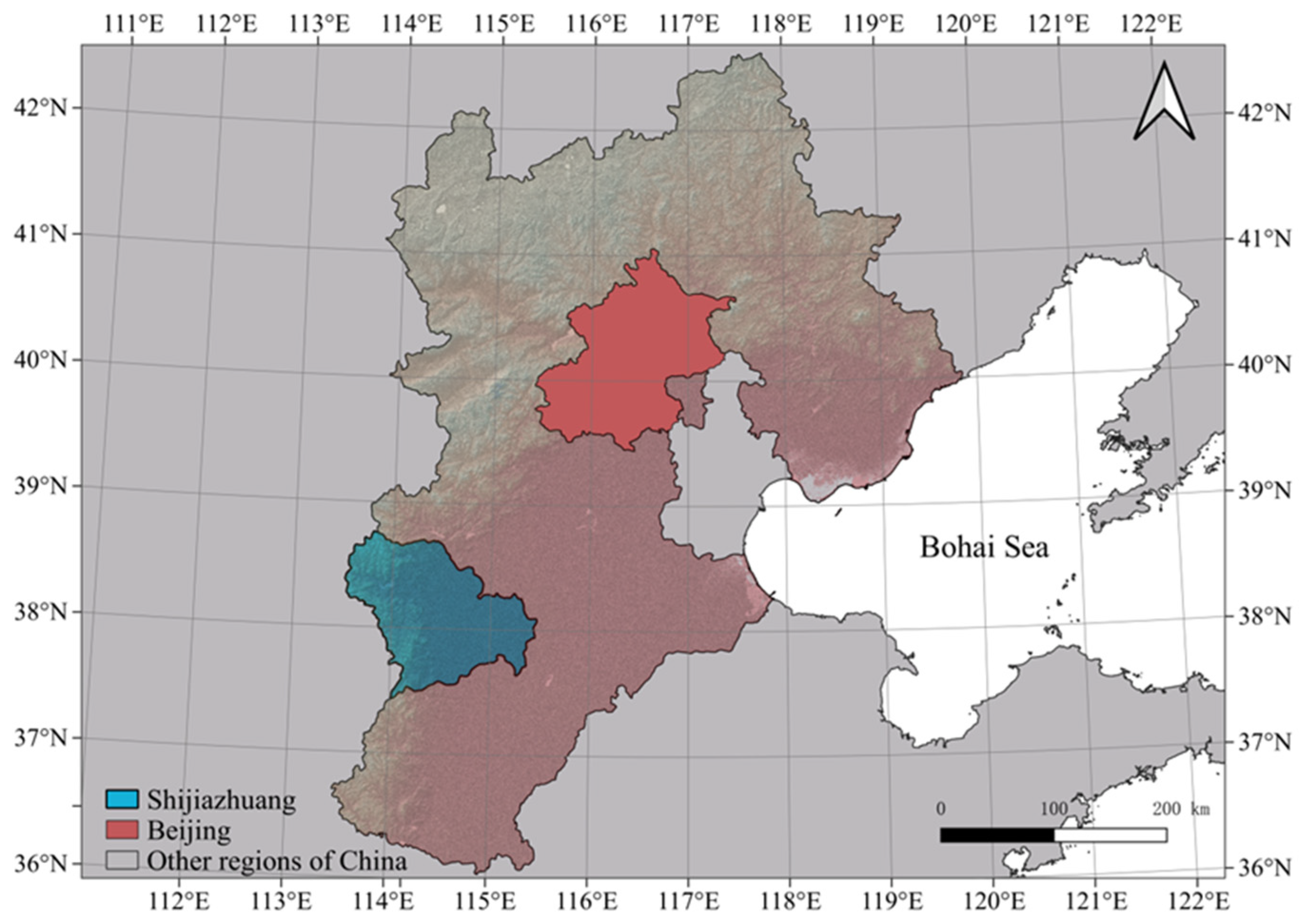
Figure 1. The map of the geographical location of Shijiazhuang City.
Atmosphere 16 01175 g001
Figure 2. Flowchart of the key-value attention mechanism.
Atmosphere 16 01175 g002
Figure 3. Flowchart of the feature attention mechanism.
Atmosphere 16 01175 g003
Figure 4. (a) 12-h, (b) 24-h, (c) 36-h, and (d) 48-h prediction results based on the BiLSTM scheme.
Atmosphere 16 01175 g004
Figure 5. (a) 12-h, (b) 24-h, (c) 36-h, and (d) 48-h prediction results based on the Feature-BiLSTM scheme.
Atmosphere 16 01175 g005
Figure 6. (a) 12-h, (b) 24-h, (c) 36-h, and (d) 48-h Prediction Results Based on the Key-Value-BiLSTM Scheme.
Atmosphere 16 01175 g006
Figure 7. (a) 12-h, (b) 24-h, (c) 36-h, and (d) 48-h prediction results based on the Dual-Attention-BiLSTM scheme.
Atmosphere 16 01175 g007
Figure 8. Comparison of prediction errors of the four models.
Atmosphere 16 01175 g008
Figure 9. Comparison of Results for Three Models.
Atmosphere 16 01175 g009
Table 1. Experiment scheme design.
Model SchemeBiLSTMFeature Attention MechanismKey-Value Attention Mechanism
Scheme 1
Scheme 2
Scheme 3
Scheme 4
Table 2. Comparison of Prediction Errors for Three Models.
TimeError Type12 h24 h36 h48 h
Model
Dual-Attention-BiLSTMRMSE1.24 °C1.17 °C1.19 °C1.37 °C
BiLSTM-KalmanRMSE1.46 °C1.18 °C1.28 °C1.18 °C
TD-LSTMRMSE1.11 °C0.89 °C0.95 °C0.88 °C
Dual-Attention-BiLSTMMAE0.90 °C0.80 °C0.92 °C1.08 °C
BiLSTM-KalmanMAE1.35 °C0.97 °C1.07 °C0.98 °C
TD-LSTMMAE0.99 °C0.74 °C0.79 °C0.70 °C
Disclaimer/Publisher’s Note: The statements, opinions and data contained in all publications are solely those of the individual author(s) and contributor(s) and not of MDPI and/or the editor(s). MDPI and/or the editor(s) disclaim responsibility for any injury to people or property resulting from any ideas, methods, instructions or products referred to in the content.