Abstract
Conventional thermospheric density models are limited in their ability to capture solar-geomagnetic coupling dynamics and lack probabilistic uncertainty estimates. We present MSIS-UN (NRLMSISE-00 with Uncertainty Quantification), an innovative framework integrating sparse principal component analysis (sPCA) with heteroscedastic neural networks. Our methodology leverages multi-satellite density measurements from the CHAMP, GRACE, and SWARM missions, coupled with MSIS-00-derived exospheric temperature (tinf) data. The technical approach features three key innovations: (1) spherical harmonic decomposition of T∞ using spatiotemporally orthogonal basis functions, (2) sPCA-based extraction of dominant modes from sparse orbital sampling data, and (3) neural network prediction of temporal coefficients with built-in uncertainty quantification. This integrated framework significantly enhances the temperature calculation module in MSIS-00 while providing probabilistic density estimates. Validation against SWARM-C measurements demonstrates superior performance, reducing mean absolute error (MAE) during quiet periods from MSIS-00’s 44.1% to 23.7%, with uncertainty bounds (1σ) achieving an MAE of 8.4%. The model’s dynamic confidence intervals enable rigorous probabilistic risk assessment for LEO satellite collision avoidance systems, representing a paradigm shift from deterministic to probabilistic modeling of thermospheric density.
1. Introduction
The thermosphere, a critical region of the space environment (~80–600 km altitude), plays a pivotal role in low Earth orbit (LEO) spacecraft operations, affecting orbital decay predictions and mission design through its dynamic variations in neutral density [1]. Characterized by pronounced spatiotemporal heterogeneity, thermospheric density fluctuations are primarily modulated by three dominant drivers: solar extreme ultraviolet (EUV) radiation, geomagnetic activity, and upward-propagating atmospheric waves from lower atmospheric layers [2]. Empirical models, such as NRLMSISE-00 [3] and JB2008 [4], parameterize solar (F10.7 index) and geomagnetic (Ap index) forcing to reproduce climatological patterns, and exhibit substantial limitations in predicting transient responses during extreme space weather events, with relative errors exceeding 200% during geomagnetic storms [5]. However, the exponential growth of LEO satellite constellations (surpassing 10,000 operational satellites by 2024) intensifies the demand for high-fidelity, robust thermospheric density models [6].
The current generation of thermospheric models suffers from inherent limitations due to oversimplified physical parameterizations. A prominent example is the NRLMSISE-00 model’s use of a single tinf to represent the thermosphere’s thermodynamic state, despite mounting observational evidence demonstrating complex latitude-local time-coupled variations in tinf that invalidate such simplified assumptions [7]. The advent of high-precision satellite accelerometry from missions including CHAMP [8], GRACE [9], and SWARM [10] has revolutionized our observational capabilities, providing unprecedented spatiotemporal resolution that has revealed critical mesoscale phenomena such as interplanetary shock-induced density perturbations [11]. These advancements have stimulated the development of novel hybrid approaches that strategically combine data-driven techniques with physical constraints.
Recent modeling breakthroughs include Pan et al.’s [12] machine learning framework that successfully integrates SWARM measurements to achieve accurate thermospheric density predictions across extended altitude ranges. Parallel developments by Turner et al. [13] have significantly advanced Reduced-Order Modeling (ROM) through the innovative incorporation of deep neural networks and autoencoder architectures, particularly convolutional deep autoencoders, which effectively capture the essential dynamics of high-dimensional density fields while enhancing both computational efficiency and predictive accuracy. Licata et al.’s [14] application of principal component analysis (PCA) to HASDM density fields demonstrated notable improvements in storm-time prediction performance. However, inherent limitations persist regarding spatial interpolation artifacts and orbital measurement correlations [15]. Despite significant progress in deep learning architectures and expanded parameter spaces, contemporary thermospheric modeling approaches remain fundamentally limited by their deterministic nature. The operational space weather forecasting community urgently requires probabilistic frameworks capable of quantifying prediction confidence intervals and error distributions—essential capabilities for reliable mission-critical applications.
Recent methodological advances have established spherical harmonic expansions as a robust mathematical framework for characterizing thermospheric variability. While Lei et al. [16] demonstrated that three principal components capture 98% of density variance at 400 km altitude using CHAMP/GRACE data, their fixed-altitude normalization approach exhibited limited cross-altitude generalizability. The dynamic reconstruction of tinf—the pivotal parameter governing thermospheric energy balance—has been identified as critical for model improvement [17]. Weimer et al. [18] advanced this paradigm by integrating NRLMSIS 2.0 for exospheric temperature-to-density conversion while incorporating spatially variable time delays between polar Poynting flux inputs and temperature responses, achieving superior predictive accuracy above 400 km during geomagnetic storms.
Persistent challenges in the field include the effective extraction of features from sparse orbital measurements, the robust quantification of uncertainty for risk assessment, and the systematic integration of physical mechanisms with data-driven approaches. To address these limitations, we propose a novel hybrid framework synergizing sPCA with probabilistic neural networks. The methodology establishes direct correspondence between in situ density measurements and tinf fields to circumvent altitude normalization artifacts, employs sparse PCA for dominant mode extraction with uncertainty quantification, and implements physics-informed deep learning for temperature mode coefficient reconstruction using solar-geomagnetic inputs and spatiotemporal features. Comparative evaluations with benchmark models (MSIS-00) across both quiet and storm conditions validate the proposed approach’s performance.
2. Data and Methodology
2.1. Satellite Data
Empirical models, such as the MSIS-00 model, compute thermospheric density through a semi-empirical approach that solves the hydrostatic equilibrium equation along the vertical column, where the temperature profile (particularly exospheric temperature) serves as the primary thermodynamic constraint. This makes tinf the pivotal parameter controlling both the magnitude and altitude distribution of density. Previous studies by Yang et al. [19], Weng et al. [20], and Ruan et al. [21] have successfully leveraged this parameter for model refinements, achieving significantly better results. In this study, we derive the effective tinf from the thermospheric densities data from the CHAMP (2002–2010), GRACE (2002–2009), and SWARM-C (2014–2020) satellites by iteratively adjusting the corresponding temperature in the empirical model without changing other inputs, until the model density matches the observed one [19]. This iterative optimization process ensures that the derived temperature accurately represents the thermospheric thermal state under different space weather conditions.
As shown in Figure 1a, the operational altitudes of the CHAMP and GRACE satellites span about 300–500 km. The comprehensive dataset captures tinf variations under different solar cycles and geomagnetic conditions. Figure 1b demonstrates that the tinf measured by the CHAMP and GRACE satellites shows excellent consistency, despite their different orbital altitudes. In addition, the temperature decreases from ~1250 K to ~650 K, corresponding to the decline of the F10.7 index from 200 sfu to 65 sfu (Figure 1c). Notably, geomagnetic disturbance significantly impacts the tinf. For instance, during the 24 August 2005 event, the 3-h Ap index peaked at 300, and the temperature surged rapidly from 740 K to 1220 K (Figure 1d subgraph), highlighting the crucial role of auroral Joule heating during geomagnetic storms.
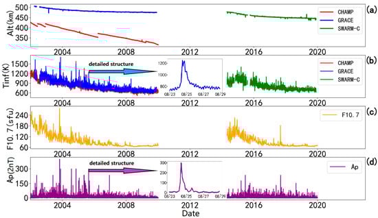
Figure 1.
(a) Variations in orbital altitudes of the CHAMP (red), GRACE-A (blue), and SWARM-C (green) satellites during the period 2002–2020; (b) tinfs derived from satellite data; (c) variations in solar F10.7 index (red) and its 81-day moving average; (d) geomagnetic Ap index.
Our modeling primarily utilizes data from the declining phase of Solar Cycle 23. At the same time, SWARM-C observations extend through the maximum and declining phases of Solar Cycle 24, providing essential validation for testing the model’s performance. These coordinated observations across multiple solar cycles substantially improve our understanding of the short-term variability and secular changes in tinf, and offer a critical insight for developing predictive thermospheric models with enhanced space weather forecasting capabilities.
2.2. Sparse Principal Component Analysis
Principal Component Analysis (PCA) is a classical data processing and dimensionality reduction technique, widely applied in meteorology and geospatial information to characterize independent physical phenomena. Principal components can be obtained through singular value decomposition of the data matrix or eigenvalue decomposition of the covariance matrix. For irregular and sparse data, such as satellite observations, directly computing the covariance matrix or performing singular value decomposition is not feasible [22]. To decompose sparse observational data, we utilize the orthogonal properties of Empirical Orthogonal Functions (EOFs) to describe the variations of satellite observations with latitude and longitude, leveraging the independence of principal components. Lei et al. [16] combined thermospheric atmospheric density results derived from CHAMP and GRACE satellite accelerometers and employed a sparse natural orthogonal function analysis method to establish an empirical model of thermospheric atmospheric density at 400 km altitude. This model quantitatively investigated the seasonal variations, particularly the annual anomaly phenomenon.
In this study, we continue to employ sparse PCA to decompose the extracted tinf data to identify dominant variation patterns using Formula (1). This decomposition yields a set of principal components represented by spherical harmonics and their corresponding temporal coefficients , which describe the spatial and temporal evolution of tinf. Herein, denote the orbit time, co-latitude, and longitude at the observation grid j (j = 1, …, J). Longitude is converted from local time. Specifically, we determine and sequentially from the first to the Pth EOF by using the least squares method [19].
The analysis reveals that the first five principal components capture 96.9% of the total variation, demonstrating their adequacy for reconstructing the tinf field. Subsequently, we develop a neural network model that takes solar radiation indices, geomagnetic activity parameters, seasonal factors, and other exospheric temperature drivers as inputs to predict the temporal coefficients associated with the principal components. The reconstructed exospheric temperature field is then obtained by combining these predicted coefficients with the principal components using Formula (1). This reconstructed temperature model is subsequently integrated into the MSIS-00 framework, replacing its original temperature calculation scheme to achieve enhanced model accuracy.
2.3. Neural Network Modeling
The temporal coefficients obtained through sparse PCA decomposition effectively capture the dynamic evolution of the principal components. Capitalizing on the well-established tinf–density relationship, we develop a probabilistic framework where uncertainty quantification in these temporal coefficients directly translates to error bounds for atmospheric density predictions. Considering the marked periodic behavior of these coefficients and their deterministic dependence on solar-geomagnetic drivers (F10.7, Ap indices), we implement a neural network architecture that assimilates processed space weather indices and auxiliary parameters to establish a robust temporal coefficient prediction system via machine learning.
2.3.1. Data Preprocessing
In this study, data preprocessing has been performed to enhance the training efficacy and prediction accuracy of the neural network model. The specific procedures include the following: (1) All input variables (F10.7 index and Ap index in Figure 2a–d) and output variables (the first-order temporal coefficient of tinf from fifth-order expansion in Figure 2f) were standardized using z-score normalization to ensure consistent scales; (2) Cyclical temporal inputs (Universal Time and day of year) were encoded via trigonometric transformations (sin encoding of day of year demonstrated in Figure 2e) to preserve their periodic characteristics. The data were partitioned into training (May 2001–June 2002, January 2003–June 2004, January 2005–June 2006, 2007–2008), validation (June–December 2002, June–December 2004, June–December 2006), and test sets (2008–2010). As shown in Figure 2c, the variation in the F10.7 index indicates that the training set encompasses a comprehensive range of high-, medium-, and low-solar-activity phases. In contrast, the deliberately isolated validation set spans independent periods with varying activity levels, facilitating unbiased hyperparameter optimization during model training.
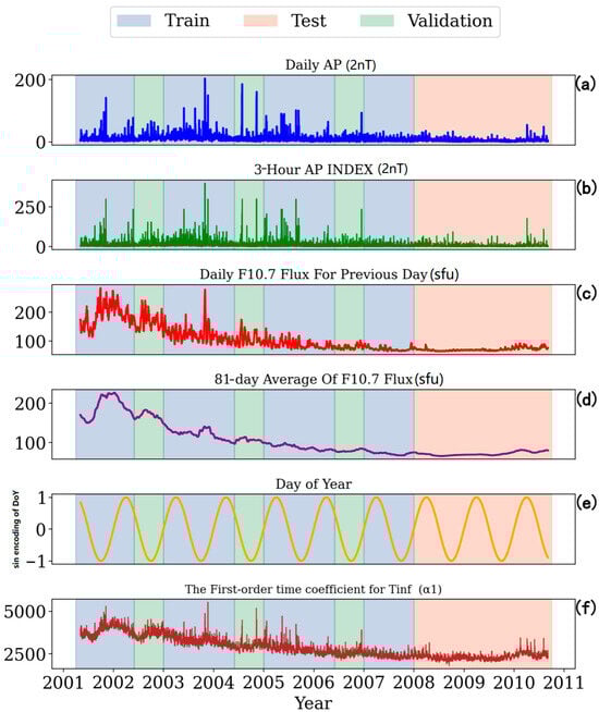
Figure 2.
Schematic of the model’s data structure: (a) the blue line represents the daily average Ap index; (b) the green line represents the 3-Hour Ap index; (c) the red line represents the daily F10.7 flux for previous day; (d) the purple line represents the 81-day average of F10.7 flux; (e) the yellow line represents the sin encoding of DoY; (f) the dark red line represents the first-order time coefficient for tinf. The light-blue shaded region indicates the training set, with light-red and light-green corresponding to the testing and validation sets, respectively.
The geomagnetic Ap index (range: 0–300) and solar F10.7 flux (range: 60–230 sfu) exhibit substantially different numerical scales, necessitating normalization for comparative analysis. To ensure consistent feature weighting, both parameters undergo linear transformation to unit magnitude (0–1 scale) while preserving their relative dynamic ranges [23]. The scaling operation employs the following formula:
Herein, denotes the raw daily F10.7 solar radio flux index and its 81-day running mean, and the 3-hourly/daily averaged geomagnetic Ap indices, respectively, while represents their scaled counterparts, and and denote the mean and standard deviation of , respectively. For the actual modeling framework, the following seven space environment parameters are utilized. Previous-day F10.7 index, 81-day averaged F10.7 index, current 3 h Ap index, 3 h Ap index at 6 h prior, 3 h Ap index at 9 h prior, current-day averaged Ap index, and previous-day averaged Ap index.
The naive scalar representation of periodic temporal features (e.g., day of year, UTC) disrupts their inherent cyclicity due to linear discontinuity. We resolve this through simultaneous sine-cosine transformations that project these features onto a unit circle ([−1, 1] range), preserving both phase continuity and gradient differentiability for neural networks [24]:
In the formulations above, and correspond to the raw day of year and Coordinated Universal Time values, respectively. The and variables denote their sine-transformed representations incorporating the first three harmonic components (i = 1–3), while and analogously represent the cosine-transformed variants. All 19 input parameters, including both space weather indices and engineered temporal features, exhibit normalized magnitudes confined to the interval [−1, 1]. This optimized scaling facilitates accelerated convergence of neural networks during training and enhances their generalization capability in prediction tasks [25].
2.3.2. Neural Network
The neural architecture in Figure 3 processes multi-scale space weather parameters (Ap index, F10.7 flux, and 81-day moving average) through a 19-node input layer that encodes solar radiative forcing, geomagnetic disturbances, and diurnal and seasonal cycles. Subsequent hidden layers (128–64 nodes) implement leaky ReLU activation (α = 0.1) [26], maintaining gradient flow (∇f(x)|x < 0 = 0.1) while circumventing neuron death. The architecture’s innovation lies in its dual-output configuration: the first five nodes perform sPCA decomposition to extract principal component coefficients. At the same time, the remaining five generate heteroscedastic uncertainty estimates, producing probabilistically calibrated predictions in the form of y ± σ. This synthesis of physically interpretable feature engineering with probabilistic deep learning enables simultaneous deterministic prediction and rigorous uncertainty quantification for space environment modeling.
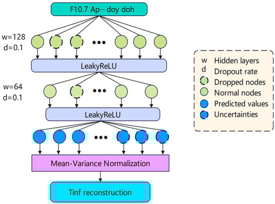
Figure 3.
Neural network architecture for modeling.
The model training incorporated Dropout regularization (retention probability p = 0.9) [27] to randomly deactivate 10% of neuronal connections during forward propagation. Through five iterations of Monte Carlo sampling iterations, this approach builds probabilistic distributions that enhance robust feature representation while suppressing overfitting. Predictive means and epistemic uncertainties are derived from sampled network evaluations, with optimization driven by a heteroscedastic loss function that simultaneously minimizes prediction target errors and uncertainty estimates, formally expressed as:
The proposed composite loss function systematically integrates three key components: the temporal coefficients () of principal components, neural network predictions (), and parametric uncertainty estimates (). This integration forms an adaptive optimization framework that inherently achieves equilibrium between predictive accuracy and uncertainty quantification. The optimization process employs the Adam algorithm with an initial learning rate (η = 0.001). It implements strict gradient clipping, specifically designed to overcome key challenges in space weather modeling [28], including gradient sparsity in non-convex landscapes, numerical instability during extreme gradient events, and pathological curvature in high-dimensional parameter spaces. This approach ensures robust performance through gradient clipping’s Lipschitz continuity bounds, adaptive moment estimation for dynamic feature learning, and guaranteed convergence under heteroscedastic noise conditions.
3. Results and Discussion
The MSIS-UN thermospheric density uncertainty model represents a significant advancement over traditional approaches by integrating neural network-derived temporal coefficients of the first five principal components with their spherical harmonic representations. This innovation fundamentally replaces the original tinf parameterization scheme in the MSIS-00 empirical model, establishing a new paradigm for simultaneously predicting thermospheric density and quantifying uncertainty. The model generates comprehensive uncertainty bounds at multiple confidence levels, with primary evaluation focused on the 68% confidence interval (μ ± 1σ), in accordance with the Three-Sigma Rule of the normal distribution. This confidence level serves as the foundational metric for assessing prediction reliability, providing robust quantification of model errors in thermospheric density estimation.
3.1. Model Performance
The neural network model demonstrates robust capability in predicting temporal coefficients of principal components along CHAMP satellite orbits, providing both coefficient estimates and their associated uncertainty ranges (±1σ, 68% confidence level). As illustrated in Figure 4, the model outputs show strong agreement with CHAMP-observed coefficients for the first four principal components during July 2009, effectively capturing multi-scale temporal variations driven by both geomagnetic activity (correlated with the Ap index) and diurnal cycles. A particularly noteworthy achievement is the model’s accurate reproduction of abrupt responses in the first, third, and fourth principal components during the geomagnetic storm at 03:00 UT on 22 July. For example, while the observed coefficient α1 peaks at ≈−0.75 approximately 7 h post-storm (10:00 UT), the model predicts a comparable peak value of −0.7 ± 0.3 at 11:00 UT, representing only a 1 h temporal offset. A comprehensive statistical analysis of 2009 predictions reveals that more than 90% of observations fall within the 68% confidence interval. This performance confirms the model’s ability to reconstruct tinf variations across spatiotemporal scales while reliably quantifying uncertainty in temporal coefficients—a critical capability for high-precision thermospheric density calculations with quantified uncertainty.
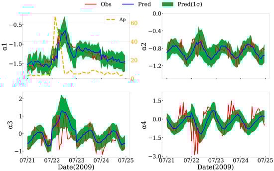
Figure 4.
Temporal coefficients of the first four tinf principal components derived from decomposition (red), alongside neural network model predictions (blue) and their uncertainty envelopes (green).
3.2. Uncertainty Quantification
The MSIS-UN atmospheric density model represents a significant methodological advancement through the integration of neural network-predicted temporal coefficients with principal components derived from sPCA. This reconstructed tinf model fundamentally replaces the conventional tinf parameterization in the MSIS-00 empirical framework, establishing a new paradigm for thermospheric density modeling with inherent uncertainty quantification capabilities. As demonstrated in Figure 5, a comparative analysis with CHAMP satellite measurements from 15 October 2005 reveals a systematic overestimation by the MSIS-00 model, while the MSIS-UN predictions show remarkable agreement with the observed tinf values. Notably, the reconstructed model not only achieves superior alignment with CHAMP density measurements but also provides reliable uncertainty bounds that encompass nearly all observational data points.
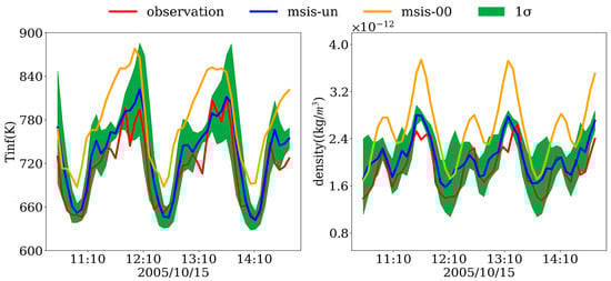
Figure 5.
Comparison of CHAMP satellite tinf (left) and thermospheric atmospheric density observations (right) with predictions from the MSIS-UN and MSIS-00 models.
To evaluate the model’s performance on the test satellite dataset, the thermospheric density along the SWARM-C satellite orbit was calculated using the MSIS-UN and MSIS-00 models. The reliability assessment of the MSIS-UN model’s uncertainty quantification is conducted through comprehensive boundary analysis and comparative error evaluation. The error calculation method is as follows:
The evaluation framework for the MSIS-UN model’s predictive capability incorporates both error analysis and uncertainty quantification. Comparative error assessment reveals that the MSIS-UN model () achieves superior accuracy over the MSIS-00 benchmark () in predicting atmospheric density () against observational data (). The model’s uncertainty bounds (: upper, : lower) demonstrate robust performance, successfully encompassing out of total data points within the predicted interval. This yields a coverage rate that quantitatively validates the model’s reliability in uncertainty characterization.
Figure 6a–c depicts the computational errors of the MSIS-UN model, the MSIS-00 model, and the MSIS-UN model at a 68% confidence level, respectively. Figure 6d illustrates the coverage of the actual atmospheric density values of the SWARM-C satellite by the MSIS-UN model at a 1σ confidence level. In the figure, ‘×’ indicates that no valid observational data is available within this interval.
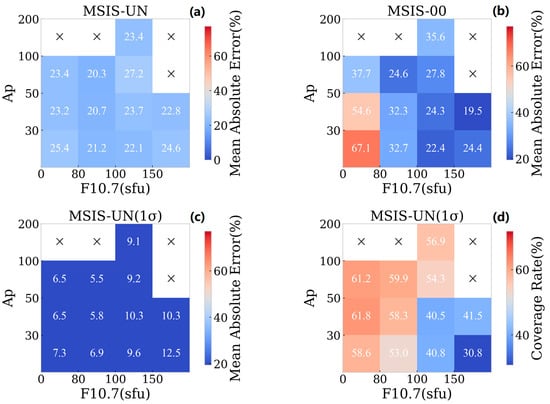
Figure 6.
Computational errors of the MSIS-UN (a), MSIS-00 (b), and MSIS-UN (c) models, along with the accurate value coverage rates (1σ) of MSIS-UN (d) under different space environment conditions.
The comprehensive evaluation reveals significant improvements in the MSIS-UN(1σ) model’s performance across varying space weather conditions. Comparative error analysis shows maximum mean errors of 24.6%, 67.1%, and 10.3% for MSIS-UN, MSIS-00, and MSIS-UN(1σ), respectively, establishing the latter’s superior computational accuracy. This advantage persists under both moderate solar activity (F10.7 < 100 sfu) and intense geomagnetic storms (Ap > 100), where the models demonstrate errors of 23.4%, 35.6%, and 9.1%, respectively. The coverage assessment further confirms the MSIS-UN(1σ) model’s enhanced reliability, with actual value coverage rates consistently exceeding 50% during both low-solar-radiation periods (peaking at 61.8%) and moderate-to-severe geomagnetic storms (Ap > 50). These results collectively demonstrate the model’s robust capability in simulating thermospheric density responses to geomagnetic disturbances, with its quantified uncertainty range effectively encompassing observed atmospheric density variations across all tested conditions.
The diurnal error patterns revealed in Figure 7 demonstrate fundamental differences in model performance characteristics. SWARM-C validation data indicate that MSIS-00 produces significantly larger daytime prediction errors (particularly in mid-to-low latitudes) compared to nighttime values, with more pronounced discrepancies in the Southern Hemisphere versus the Northern Hemisphere. In contrast, MSIS-UN exhibits an inverse diurnal pattern, achieving superior daytime accuracy but showing elevated nighttime errors, concentrated in mid-latitude regions—a phenomenon potentially linked to its limited capacity in modeling midnight equatorial density anomalies.
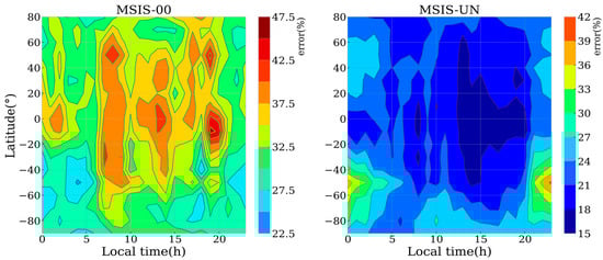
Figure 7.
Errors versus the geographic latitude and local time between the densities from MSIS-00 and MSIS-UN predictions and the SWARM-C observations.
Comparative analysis establishes MSIS-UN’s overall superiority, with its maximum error (42%) substantially lower than MSIS-00’s peak discrepancy (47.5%). The only exception occurs in Southern Hemisphere mid-latitudes during nighttime conditions, where MSIS-00 maintains a marginal advantage. This comprehensive evaluation confirms MSIS-UN’s enhanced predictive capability across most spatial and temporal domains, while identifying specific regions that require further refinement of the model.
Comparative performance evaluation across geomagnetic activity levels reveals systematic improvements in the MSIS-UN model’s predictive capability. As detailed in Table 1, during geomagnetically quiet conditions (Ap ≤ 30), MSIS-UN exhibits statistically significant accuracy enhancements compared to MSIS-00. This performance advantage persists through minor (30 < Ap ≤ 50) and significant geomagnetic storms (Ap > 50), with both models showing progressively improved precision as geomagnetic activity intensifies—a phenomenon potentially attributable to either data sparsity during storm events or the robust storm-response parameterizations inherent in both model architectures.

Table 1.
MAE and true value coverage rates of the MSIS-00, MSIS-UN, and MSIS-UN at the 1σ confidence level models.
The quantitative superiority of MSIS-UN is evidenced by its substantially lower overall average relative error (23.7%) compared to MSIS-00 (44.1%). Most notably, the 1σ confidence-level implementation achieves exceptional performance metrics, combining an 8.4% computational error with a 50.0% actual value coverage rate. These results collectively validate MSIS-UN’s advanced capability in both atmospheric density prediction and uncertainty quantification across the full spectrum of geomagnetic activity conditions.
3.3. Geomagnetic Storm Evaluation
The validation study of two major geomagnetic storms (Kp = 9) that occurred on 8 September 2017 and 27 August 2018 reveals distinct performance characteristics in the MSIS-UN and MSIS-00 models. During the September 2017 event (Figure 8a), MSIS-UN demonstrates superior accuracy in simulating pre-storm tinf and atmospheric density along the SWARM-C satellite orbit, while MSIS-00 exhibits systematic overestimation exceeding 40%. The first storm phase shows temperature increases from 824K to 960K, with MSIS-UN (1047K, 9% error) significantly outperforming MSIS-00 (1335K, 39% error). The second storm phase reveals that both models accurately capture the 1118K temperature enhancement, with MSIS-UN’s predicted range fully encompassing the observed densities.
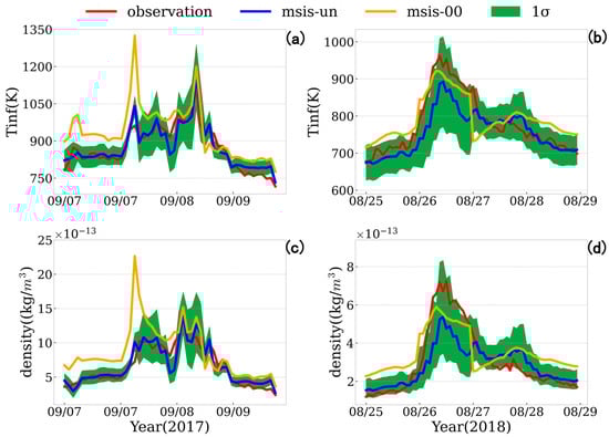
Figure 8.
Comparison of (a,c) tinf and atmospheric density observed by SWARM-C (red lines) during the 2017 geomagnetic storms, and (b,d) corresponding 2018 storm events, with model predictions from MSIS-00 (yellow lines), MSIS-UN (blue lines), and MSIS-UN 1σ uncertainty bounds (green bands).
The August 2018 event (Figure 8b,d) presents more complex patterns. While maintaining MSIS-00’s characteristic overestimation in pre-storm conditions, the geomagnetic storm drives observed temperatures from 659K to 960K. Notably, MSIS-00’s systematic bias paradoxically results in closer absolute density values during peak storm conditions despite larger relative errors in storm response simulation. Conversely, MSIS-UN underestimates main-phase density by ~25% but achieves superior accuracy in both pre-storm and recovery phases. Crucially, MSIS-UN’s predicted density range consistently encompasses accurate observations throughout both events, demonstrating robust uncertainty quantification capabilities.
A comparative analysis of Figure 8c confirms that MSIS-UN’s improved atmospheric density response simulation during geomagnetic storms yields predictions that show strong consistency with tinf variations and comprehensive coverage of observed values, marking a notable improvement over MSIS-00’s persistent overestimation patterns. These results collectively establish MSIS-UN’s advanced capability in both storm-time thermospheric density prediction and uncertainty range quantification.
4. Summary
The proposed MSIS-UN framework represents a significant advancement in thermospheric density modeling, due to its innovative integration of machine learning with robust uncertainty quantification. Validation against SWARM satellite observations demonstrates substantial improvements over the conventional MSIS-00 model, with MSIS-UN achieving a MAE of 23.7% in density predictions compared to MSIS-00’s 44.1% error. At the 68% confidence level, the model’s predictive intervals demonstrate remarkable reliability, encompassing 50.0% of the observed densities with only 8.4% computational error.
Performance evaluation across diverse space weather conditions demonstrates consistent superiority, particularly during geomagnetic storms and periods of low solar activity. The model accurately captures storm-time density enhancements during both the primary and recovery phases, outperforming MSIS-00 in terms of temporal response characteristics and magnitude estimation. This enhanced capability stems from the machine learning architecture’s inherent capacity to capture nonlinear thermospheric responses to external forcing.
Future development pathways focus on three strategic dimensions: incorporating emerging LEO constellation datasets to enhance spatial coverage, implementing advanced machine learning techniques (including deep neural networks and ensemble methods) to refine prediction accuracy, and establishing a unified global prediction framework. These enhancements aim to further bridge the gap between empirical modeling and first-principles simulations, potentially revolutionizing thermospheric research and space weather forecasting capabilities.
Author Contributions
Conceptualization of the Manuscript Idea: J.L., X.N. and Y.W.; Methodology and Software: J.L., Y.W. and X.N.; Writing Original Draft: J.L.; Writing—Review: Y.W. All authors have read and agreed to the published version of the manuscript.
Funding
This work is supported by the National Natural Science Foundation of China (Grants 42441828, and 42474219), the Shandong Provincial Natural Science Foundation (Grant ZR2022MD034), the Stable-Support Scientific Project of China Research Institute of Radiowave Propagation (Grant A241204230), Xiaomi Young Talents Program.
Institutional Review Board Statement
Not applicable.
Informed Consent Statement
Not applicable.
Data Availability Statement
Thermospheric density data from the CHAMP, GRACE, and SWARM-C satellites are available at http://thermosphere.tudelft.nl (accessed on 13 March 2021).
Acknowledgments
The authors are grateful to the sponsors and operators of the CHAMP, GRACE, and SWARM missions.
Conflicts of Interest
The authors declare no conflicts of interest.
References
- Emmert, J.T. Thermospheric Mass Density: A Review. Adv. Space Res. 2015, 56, 773–824. [Google Scholar] [CrossRef]
- Liu, H.; Lühr, H. Strong disturbance of the upper thermospheric density due to magnetic storms: CHAMP observations. J. Geophys. Res. Space Phys. 2005, 110, A9. [Google Scholar] [CrossRef]
- Picone, J.M.; Hedin, A.E.; Drob, D.P.; Aikin, A.C. Nrlmsise-00 Empirical Model of the Atmosphere: Statistical Comparisons and Scientific Issues. J. Geophys. Res. Space Phys. 2002, 107, 1468. [Google Scholar] [CrossRef]
- Bowman, B.R.; Tobiska, W.K.; Marcos, F.A.; Huang, C.; Lin, C.; Burke, W. A New Empirical Thermospheric Density Model JB2008 Using New Solar and Geomagnetic Indices; American Institute of Aeronautics and Astronautics: Honolulu, HI, USA, 2008. [Google Scholar]
- Bruinsma, S. The Dtm-2013 Thermosphere Model. J. Space Weather Space Clim. 2015, 5, A1. [Google Scholar] [CrossRef]
- Newman, C.J.; Williamson, M. Space Sustainability: Reframing the Debate. Space Policy 2018, 46, S0265964617300462. [Google Scholar] [CrossRef]
- Park, J.; Evans, J.S.; Eastes, R.W.; Lumpe, J.D.; Ijssel, J.v.D.; Englert, C.R.; Stevens, M.H. Exospheric Temperature Measured by Nasa-Gold under Low Solar Activity: Comparison with Other Data Sets. J. Geophys. Res. Space Phys. 2022, 127. [Google Scholar] [CrossRef]
- Doornbos, E.; Klinkrad, H.; Visser, P. Atmospheric density calibration using satellite drag observations. Adv. Space Res. 2005, 36, 515–521. [Google Scholar] [CrossRef]
- Sutton, E.K. Normalized Force Coefficients for Satellites with Elongated Shapes. J. Spacecr. Rocket. 2009, 46, 112–116. [Google Scholar] [CrossRef]
- Siemes, C.; de Teixeira da Encarnação, J.; Doornbos, E.; Ijssel, J.v.D.; Kraus, J.; Pereštý, R.; Grunwaldt, L.; Apelbaum, G.; Flury, J.; Olsen, P.E.H. Swarm accelerometer data processing from raw accelerations to thermospheric neutral densities. Earth Planets Space 2016, 68, 1–18. [Google Scholar] [CrossRef]
- Zesta, E.; Oliveira, D.M. Thermospheric Heating and Cooling Times During Geomagnetic Storms, Including Extreme Events. Geophys. Res. Lett. 2019, 46, 12739–12746. [Google Scholar] [CrossRef]
- Pan, Q.; Xiong, C.; Lühr, H.; Smirnov, A.; Huang, Y.; Xu, C.; Yang, X.; Zhou, Y.; Hu, Y. Machine learning based modeling of the thermospheric mass density. Space Weather 2024, 22, e2023SW003844. [Google Scholar] [CrossRef]
- Turner, H.; Zhang, M.; Gondelach, D.; Linares, R. Machine Learning Algorithms for Improved Thermospheric Density Modeling. In Dynamic Data Driven Applications Systems; DDDAS 2020. Lecture Notes in Computer Science; Darema, F., Blasch, E., Ravela, S., Aved, A., Eds.; Springer: Cham, Switzerland, 2020; Volume 12312. [Google Scholar] [CrossRef]
- Licata, R.J.; Mehta, P.M.; Tobiska, W.K.; Huzurbazar, S. Machine learned HASDM thermospheric mass density model with uncertainty quantification. Space Weather 2022, 20, e2021SW002915. [Google Scholar] [CrossRef]
- Licata, R.J.; Mehta, P.M.; Weimer, D.R.; Tobiska, W.K. Improved Neutral Density Predictions through Machine Learning Enabled Exospheric Temperature Model. Space Weather 2021, 19, e2021SW002918. [Google Scholar] [CrossRef]
- Lei, J.; Matsuo, T.; Dou, X.; Sutton, E.; Luan, X. Annual and Semiannual Variations of Thermospheric Density: Eof Analysis of Champ and Grace Data. J. Geophys. Res. Space Phys. 2012, 117. [Google Scholar] [CrossRef]
- Yiğit, E.; Knížová, P.K.; Georgieva, K.; Ward, W. A review of vertical coupling in the atmosphere-ionosphere system: Effects of waves, sudden stratospheric warmings, space weather, and of solar activity. J. Atmos. Sol.-Terr. Phys. 2016, 141, 1–12. [Google Scholar] [CrossRef]
- Weimer, D.R.; Tobiska, W.K.; Mehta, P.M.; Licata, R.J.; Drob, D.P.; Yoshii, J. Comparison of a Neutral Density Model with the Set Hasdm Density Database. Space Weather 2021, 19, e2021SW002888. [Google Scholar] [CrossRef]
- Yang, X.; Zhu, X.; Weng, L.; Yang, S. A New Exospheric Temperature Model Based on CHAMP and GRACE Measurements. Remote Sens. 2022, 14, 5198. [Google Scholar] [CrossRef]
- Weng, L.; Lei, J.; Sutton, E.; Dou, X.; Fang, H. An Exospheric Temperature Model from Champ Thermospheric Density. Space Weather 2017, 15, 343–351. [Google Scholar] [CrossRef]
- Ruan, H.; Lei, J.; Dou, X.; Liu, S.; Aa, E. An Exospheric Temperature Model Based on Champ Observations and Tiegcm Simulations. Space Weather 2018, 16, 147–156. [Google Scholar] [CrossRef]
- Matsuo, T.; Richmond, A.D.; Nychka, D.W. Modes of High-Latitude Electric Field Variability Derived from De-2 Measurements: Empirical Orthogonal Function (Eof) Analysis. Geophys. Res. Lett. 2002, 29, 7. [Google Scholar] [CrossRef]
- Yuan, L.; Jin, S.; Calabia, A. Distinct thermospheric mass density variations following the September 2017 geomagnetic storm from GRACE and Swarm. J. Atmos. Sol.-Terr. Phys. 2019, 184, 30–36. [Google Scholar] [CrossRef]
- Mirjalili, S. SCA: A Sine Cosine Algorithm for Solving Optimization Problems. Knowl.-Based Syst. 2016, 96, 120–133. [Google Scholar] [CrossRef]
- Sidorenko, K.A.; Kondratyev, A.N. Improving the ionospheric model accuracy using artificial neural network. J. Atmos. Sol.-Terr. Phys. 2020, 211, 105453. [Google Scholar] [CrossRef]
- Maas, A.L.; Hannun, A.Y.; Ng, A.Y. Rectifier nonlinearities improve neural network acoustic models. In Proceedings of the ICML Workshop on Deep Learning for Speech and NLP, Atlanta, GA, USA, 16–21 June 2013. [Google Scholar]
- Gal, Y.; Ghahramani, Z. Dropout as a Bayesian approximation: Representing model uncertainty in deep learning. In Proceedings of the International Conference on Machine Learning (ICML), New York, NY, USA, 19–24 June 2016. [Google Scholar]
- Kingma, D.; Ba, J. Adam: A Method for Stochastic Optimization. arXiv 2014, arXiv:1412.6980. [Google Scholar] [CrossRef]
Disclaimer/Publisher’s Note: The statements, opinions and data contained in all publications are solely those of the individual author(s) and contributor(s) and not of MDPI and/or the editor(s). MDPI and/or the editor(s) disclaim responsibility for any injury to people or property resulting from any ideas, methods, instructions or products referred to in the content. |
© 2025 by the authors. Licensee MDPI, Basel, Switzerland. This article is an open access article distributed under the terms and conditions of the Creative Commons Attribution (CC BY) license (https://creativecommons.org/licenses/by/4.0/).