Forecasting Indoor Air Quality in Mexico City Using Deep Learning Architectures

Abstract

Air pollution causes millions of premature deaths per year due to its strong association with several diseases and respiratory afflictions. Consequently, air quality monitoring and forecasting systems have been deployed in large urban areas. However, those systems forecast outdoor air quality while people living in relatively large cities spend most of their time indoors. Hence, this work proposes an indoor air quality forecasting system, which was trained with data from Mexico City, and that is supported by deep learning architectures. The novelty of our work is that we forecast an indoor air quality index, taking into account seasonal data for multiple horizons in terms of minutes; whereas related work mostly focuses on forecasting concentration levels of pollutants for a single and relatively large forecasting horizon, using data from a short period of time. To find the best forecasting model, we conducted extensive experimentation involving 133 deep learning models. The deep learning architectures explored were multilayer perceptrons, long short-term memory neural networks, 1-dimension convolutional neural networks, and hybrid architectures, from which LSTM rose as the best-performing architecture. The models were trained using (i) outdoor air pollution data, (ii) publicly available weather data, and (iii) data collected from an indoor air quality sensor that was installed in a house located in a central neighborhood of Mexico City for 17 months. Our empirical results show that deep learning models can forecast an indoor air quality index based on outdoor concentration levels of pollutants in conjunction with indoor and outdoor meteorological variables. In addition, our findings show that the proposed method performs with a mean squared error of 0.0179 and a mean absolute error of 0.1038. We also noticed that 5 months of historical data are enough for accurate training of the forecast models, and that shallow models with around 50,000 parameters have enough predicting power for this task.

1. Introduction

Air pollution has been associated with chronic respiratory diseases [1], cardiovascular diseases [2], Parkinson’s disease [3], and increased mortality [4]. In fact, it is estimated that, worldwide, each year there are 3 million premature deaths caused by air pollution [5]. In addition, there is evidence that a reduction in air pollution is linked to an increase in life expectancy [6]. For the above reasons, recent years have witnessed the awakening of various concerns about air pollution and its negative effects on human health; see, for instance, [7]. Within this domain, a particular topic of interest is the monitoring and forecasting of air quality in large urban areas (see [8] for an overview of monitoring and forecasting techniques).

In general, air quality monitoring systems [9] focus on specific components known for their adverse impact on human health, among which are nitrogen dioxide (${\mathrm{NO}}_2$), ozone (${\mathrm{O}}_3$), carbon monoxide (CO), and particulate matter (${\mathrm{PM}}_{10}$, ${\mathrm{PM}}_{2.5}$). Concentration measurements of these pollutants (and others) are grouped, transformed, and summarized into air quality indexes [10], which categorize air quality in levels (comprehensible to the average person) ranging from good to hazardous, as in the air quality index reported in [11,12]. Historically, air quality studies have focused on outdoor air quality [13,14,15,16,17]. However, as reported in [18,19,20], people living in urban areas of developed countries spend over 90% of their time indoors. In addition, despite the negative impact that outdoor air pollutants have on indoor air quality [21,22] and the relevance of indoor air quality to human health, indoor air quality monitoring and forecasting have received considerably less attention [23], with a few exceptions focused on indoor air quality in relatively crowded buildings such as senior centers [24], schools [25], and public buildings [26].

In this work, we investigate the potential of using deep learning models for the forecasting of indoor air quality. We built and evaluated 133 different deep learning-based forecasting models to predict an indoor air quality index (IAQ), based on the United States Environmental Protection Agency’s air quality index [11]. The motivation for evaluating deep learning models on this task is because these models have become the state of the art for dealing with non-linear problems, which is the case for predicting indoor air quality from outdoor records. More precisely, the scientific problem that we face consists in finding a (non-linear) function able to forecast indoor air quality from both outdoor and indoor records of different pollutants and environmental variables. Our objective is to obtain predictions as accurately as possible, such that we could help keep people informed about indoor air quality. Three commonly used deep learning architectures were combined and evaluated in order to select the best-performing model. The neural network architectures involved were (i) dense neural networks (DNNs), also known as fully connected neural networks or multilayer perceptrons, which are the basis for other neural networks architectures and also commonly used for forecasting [27]; (ii) long short-term memory (LSTM) neural networks, which are widely used for time-series data [28]; and (iii) 1-dimension convolutional neural networks (CNNs), which are also commonly used for time-series modeling, e.g., [29]. These deep learning architectures were trained using three complementary sources of data: (i) records of outdoor air pollution (provided by a Mexican government agency) [30]; (ii) publicly available weather data (provided by OpenWeather [31]); and (iii) data collected from an indoor air quality sensor [12]. This work contributes an indoor air quality forecasting system supported by deep learning models with an MSE of 0.0179 and a mean absolute error (MAE) of 0.1038. This contribution involved collecting and curating data of over 17 months of indoor and outdoor air quality records from three different data sources. The novelty and relevance of this work is that, to the best of our knowledge, it is among the earliest deep learning approaches in forecasting an indoor air quality index for Mexico City based on indoor and outdoor features that takes into account seasonal data.

2. Related Work

Previous work has focused on forecasting (or classifying) outdoor concentration levels of common pollutants (see [32,33]) and outdoor air quality indexes (see [34]). Other works have focused on identifying the source affecting indoor air quality (see [35]) and forecasting indoor concentration levels of pollutants (see [36,37,38,39]). Yet, despite the relevance of indoor air quality to human health [40], only a few works have focused on forecasting indoor air quality indexes, e.g., [41] and our present research effort. These works and our present work are characterized in Table A1 (in Appendix A) and discussed below.

Abdullah et al. [32] highlighted both (i) the complexity of forecasting outdoor concentration levels of common pollutants due to vehicular traffic, and (ii) the non-linear relationships among meteorological variables, traffic-related variables, and air quality (as measured by the outdoor concentration level of pollutants). Due to this complexity, Abdullah et al. [32] proposed a multilayer perceptron (MLP) neural network model enhanced with a genetic algorithm to update weights, which they called an optimized artificial neural network. By making use of meteorological, air pollution, and vehicular traffic databases of Kuala Lumpur, Malaysia, they trained their optimized neural network to produce a 1 h forecast of outdoor concentration levels of CO, NO, ${\mathrm{NO}}_2$, and ${\mathrm{NO}}_{\mathrm{x}}$. According to their experiments, their optimized artificial neural network outperformed a regular MLP, a decision tree model, and a random forest model. In our work, we have kept the idea of using non-linear transformations inside artificial neural networks as forecasting models (as it is currently a common practice). However, we have relied on the back-propagation algorithm for the optimization of our models, as it is the current state of the art.

Using a database of hourly and daily concentration levels of air pollutants in Nicosia, Cyprus, Cakir and Sita [33] trained MLPs to forecast outdoor concentration levels of ${\mathrm{O}}_3$, ${\mathrm{PM}}_{10}$, and ${\mathrm{NO}}_2$ for each season (namely, winter, spring, summer, and fall) and compared them against multiple linear regression models (also built for each season). Cakir and Sita [33] found that, in general, the multiple linear regression models outperformed the MLPs. However, they also found that for some seasons and pollutants, the MLPs yielded better results than the multiple linear regression models. It is worth mentioning that by building multiple linear regression models for each season Cakir and Sita [33] may have reduced the need for non-linear models such as (deep) neural networks. In our work, based on the non-linear relationships highlighted by Abdullah et al. [32], we have built deep neural network models and excluded linear models. In addition, unlike Cakir and Sita [33], we trained deep neural networks taking into all seasons, i.e., without building forecasting models for each season.

In contrast to Abdullah et al. [32] and Cakir and Sita [33] that forecast outdoor concentration levels of pollutants, Shukla et al. [34] classified concentration levels of 12 pollutants (of multiple Indian cities) into an outdoor air quality index. One of the main contributions of Shukla et al. [34] is the use of an artificial neural network in conjunction with linear vector quantization to classify the concentration levels of the pollutants into the outdoor air quality index attaining an accuracy of 97.59%. Their promising results are attributed to updating weights using linear vector quantization. Whereas Shukla et al. [34] classified pollutants’ concentration levels into good, moderate, poor, satisfactory, severe, and very poor, in our present work, we have forecast an indoor air quality index represented by a scalar using meteorological variables and concentration levels of pollutants.

Another important study on air quality was carried out by Saad et al. [35], who focused on identifying/classifying the source affecting indoor air quality. The potential sources explored were ambient air, chemical presence, fragrance presence, food and beverages, and human activity. Saad et al. [35] trained an MLP using features such as temperature, relative humidity, volatile organic compounds, and common pollutants (${\mathrm{CO}}_2$, CO, ${\mathrm{O}}_3$, ${\mathrm{NO}}_2$, ${\mathrm{O}}_2$, ${\mathrm{PM}}_{10}$). It should be highlighted that their model achieved an accuracy of 99.1%. As Saad et al. [35], in this present work, we made use of MLPs in addition to other deep learning methods. Moreover, whereas the features used by Saad et al. [35] and ours are similar, Saad et al. [35]’s work and ours differ in objective. In fact, we believe that our indoor air quality forecasting system can be complemented by a system to detect the source affecting air quality (such as the one proposed by Saad et al. [35]).

Also, in the domain of indoor air quality, but specialized for buildings, Kapoor et al. [36] focused on forecasting the concentration level of carbon dioxide ($\mathrm{C}{\mathrm{O}}_2$) in an office using several machine learning algorithms. Their pilot study was carried out in a research laboratory located in Roorkee, India. The models were built using features such as number of room occupants, office area, temperature, relative humidity, wind speed, and an indoor air quality index. Their best-performing model was a Gaussian process regression, achieving an RMSE of 4.2006 and an MAE of 3.3509. Instead of forecasting a concentration level of a single pollutant (as in [36]), in this work, we have built (and evaluated) a system capable of forecasting an indoor air quality index, which results from a combination of pollutants. In addition, our deep learning models were trained and evaluated using data from different seasons since we collected data for 17 months, unlike Kapoor et al. [36], who built and evaluated their models using data from only one month.

Ahn et al. [37] built multiple models to forecast indoor temperature, indoor relative humidity, indoor level of fine dust, indoor light quantity, and indoor concentration levels of volatile organic compounds. They made use of linear regressions, gated recurrent unit networks, and LSTM neural networks. Whereas their worst results were obtained using a linear regression model, the best forecasting results were obtained using gated recurrent unit networks and LSTM neural networks, although the best-performing model was a gated recurrent unit network. Unfortunately, Ahn et al. [37] evaluated their results using non-standard forecast metrics, in particular using a custom metric based on classification accuracy that was adapted to evaluate forecasts, which makes comparison unfeasible. Also, in contrast to our models that were built using data from different seasons, their models were built using 7 months of data, which may have left out some seasonal patterns.

As in our present work, Bakht et al. [38] made use of deep learning models to forecast indoor air quality (as measured by concentration levels of ${\mathrm{PM}}_{10}$ and ${\mathrm{PM}}_{2.5}$) in the context of subway stations. To forecast air quality, they made use of MLPs, (bidirectional) LSTMs, recurrent neural networks, CNNs, and a hybrid CNN-LSTM-MLP neural network, which yielded the best results (namely an RMSE of 8.94 and an MAE of 6.4). As in our present work, Bakht et al. [38] trained their models using features related to indoor and outdoor concentration levels of common pollutants; however, we also made use of meteorological features.

Also using LSTM neural networks, Sharma et al. [39] built IndoAirSense (a system for indoor air quality forecasting). In addition to features related to common pollutants, they also collected data about the number of room occupants, room size, and the number of fans in the room. Firstly, to forecast indoor air quality, they used an MLP to estimate concentration levels of pollutants that served as input to different variants of LSTM neural networks, which forecast indoor concentration levels of ${\mathrm{CO}}_2$ and ${\mathrm{PM}}_{2.5}$. Sharma et al. [39] built and evaluated an LSTM, a bidirectional LSTM, a deep bidirectional and unidirectional LSTM, and a modified LSTM without forget gates, which was the best-performing model with an MAPE of 4%. It should be noted that their models were built and evaluated using data from only one month, which may have left out some seasonal patterns. As in [39], in this present work, we also identified the potential of LSTM neural networks to forecast indoor air quality; however, unlike Sharma et al. [39] that forecast indoor concentration levels of pollutants, we have forecast an indoor air quality index.

Among the related work discussed in this section, in terms of target variables, the work by Rastogi et al. [41] is highly related to our present work. Rastogi et al. [41] built a discrete-time Markov chain model capable of forecasting return times to states associated with an indoor air quality index. In contrast, our present work does not forecast return times to index states but an indoor air quality index. To build their model, Rastogi et al. [41] collected data on indoor concentration levels of CO, ${\mathrm{PM}}_{10}$, and ${\mathrm{PM}}_{2.5}$, and a (lagged) indoor air quality index for 13 months in Delhi, India. In addition to those input variables, in our present work, we also collected data about other common pollutants and meteorological variables. Unfortunately, we did not find their data, source code, nor sufficient technical detail to replicate their results.

In summary, either in the case of indoor or outdoor air quality forecasting, comparing the performance of forecasting models is quite difficult and may be unfeasible due to the use of different metrics, different input variables, different target variables, different data collection time frames, different geographic areas of interests, and different techniques. Having said that, however, as discussed in Section 4, our proposed indoor air quality forecasting system achieved an MSE of 0.0179 and an MAE of 0.1038, which are comparable to the performance of other forecasting models (see Table A1). This gives evidence for the potential usefulness of our indoor air quality forecasting system supported by a deep learning model. In addition, except for Rastogi et al. [41], all the other research efforts (discussed in this section), and our present work, made use of (deep) artificial neural networks to forecast a target variable related to air quality. Also, as reported in Table A1, our present work is among the few that built and evaluated deep learning models using data including samples from different seasons, which is important because air pollution (in relatively large cities) is seasonal [42]. A key difference between our present work and the related work (discussed in this section) is that it is the only research effort forecasting an indoor air quality index, although Rastogi et al. [41] forecast return times to states associated with an indoor air quality index. Moreover, our present work is among the few (see Table A1) building and evaluating forecasting models for multiple horizons in terms of minutes. Furthermore, in contrast to [32,33,34,35,36,37,38,39,41], our proposed experimental methodology (see Section 3) allowed us to build and evaluate up to 133 deep learning models using automated cloud resource orchestration and parallel hyperparameter tuning.

It is acknowledged that this present work is a significantly extended version of a preliminary work presented in [43]. Whereas in [43] we built and evaluated only 10 neural network models trained with 8 months of data, in this present work, we conducted extensive experimentation involving 133 deep learning models (even including hybrid models), which were trained with 17 months of data. In addition, in this present work, we have (i) extended and deepened the related work comparison; (ii) considerably enhanced the exploratory data analysis by exploring seasonal patterns, conducting auto-correlation as well as partial auto-correlation analyses, and exploring cross-correlations between the target and independent variables; (iii) implemented a data pipeline for preprocessing the time-series data and automated hyperparameter optimization and model training using Google Vertex AI; and (iv) included and discussed completely new results derived from the evaluation of the 133 deep learning models.

3. Materials and Methods

The materials used for the proposed indoor air quality forecasting system were as follows:

• A Bosch BME680 indoor air quality sensor, which was manufactured in Berlin, Germany in 2009 by Bosch. Additional details can be found in [12].
• A data storage device that gathers and stores the observations from the indoor air quality sensor.
• A set of computing resources for data preprocessing and model training (Section 3.1).
• Data from the indoor air quality sensor and external sources (see Section 3.2, Section 3.3, Section 3.4 for details).

The methods used in this research effort (Figure 1) were as follows:

• Collecting air quality data for 17 months (Section 3.2).
• An exploratory data analysis for time-series data (Section 3.4).
• Data cleansing and data transformations (Section 3.5).
• Deep neural network architectures (Section 3.6).
• Model training and evaluation (Section 3.7).

Figure 1. Deep learning forecasting methodology.

3.1. Computing Environment

Our experiments were conducted on Google’s Vertex AI platform using T4 GPUs. We used the Python programming language, in particular, TensorFlow, a platform for machine learning.

3.2. Data Collection

We collected data using a Bosch BME680 sensor that measures humidity, pressure, and temperature and reports an indoor air quality index [11]. The sensor was located in a central neighborhood of Mexico City at coordinates 19°28′19.2″ N 99°09′32.4″ W. In particular, the sensor was located in the middle of the main room of a house at a height of 2.2 m and away from (i) direct ventilation and (ii) sources of volatile organic compounds, in order to collect reliable data every 3 s. The data collected from the sensor were stored in a second-generation Raspberry Pi.

In addition to the data collected from the indoor air quality sensor, we used two external data sources: (i) OpenWeather [31], that reports weather data; and (ii) SINAICA, a Mexican government agency that reports data on outdoor air pollution [30]. The data from both OpenWeather and SINAICA are publicly available and were gathered within a 10 km radius from the indoor air quality sensor. It should be noted that, based on an exploratory data analysis, we detected that data collected from the external data sources had some missing values. For this reason, we only used the monitoring stations and pollutants with the least number of missing values. The full data set comprises 532 days of air quality records, i.e., over 17 months of data from 12 February 2021 to 28 July 2022.

3.3. Data Input and Target Variables

The deep learning models for indoor air quality forecasting were trained using the following variables (grouped by data source type):

• Data variables collected from a Bosch BME680 sensor:

  -

  Indoor air quality index (IAQ): a discrete variable corresponding to the United States Environmental Protection Agency’s air quality index [11].

  -

  Indoor temperature: a continuous variable in Celsius degrees.

  -

  Indoor pressure: a continuous variable in hectopascals (hPa).

  -

  Indoor relative humidity: a continuous variable expressed as a percentage.

• Data variables collected from SINAICA:

  -

  Outdoor NO: a continuous variable for nitric oxide in parts per billion (ppb).

  -

  Outdoor ${\mathrm{NO}}_2$: a continuous variable for nitrogen dioxide in ppb.

  -

  Outdoor ${\mathrm{NO}}_{\mathrm{x}}$: a continuous variable for nitrogen oxide in ppb.

  -

  Outdoor CO: a continuous variable for carbon monoxide in ppb.

  -

  Outdoor ${\mathrm{O}}_3$: a continuous variable for ozone in ppb.

  -

  Outdoor ${\mathrm{PM}}_{10}$: a continuous variable for particle matter with a diameter of less than 10 microns expressed in micrograms per cubic meter ($\mathsf{\mu }$${\mathrm{g/m}}^3$).

  -

  Outdoor ${\mathrm{PM}}_{2.5}$: a continuous variable for particle matter with a diameter of less than 2.5 microns expressed in μg/m³.

  -

  Outdoor ${\mathrm{SO}}_2$: a continuous variable for sulfur dioxide in ppb.

• Data variables collected from OpenWeather:

  -

  Outdoor temperature: a continuous variable in Celsius degrees.

  -

  Outdoor pressure: a continuous variable in hPa.

  -

  Outdoor relative humidity: a continuous variable expressed as a percentage.

Whereas the output of the deep learning models corresponds to the IAQ (the target variable), the input corresponds to all the remaining variables, i.e., no lagged observations of the IAQ are used as input to the models.

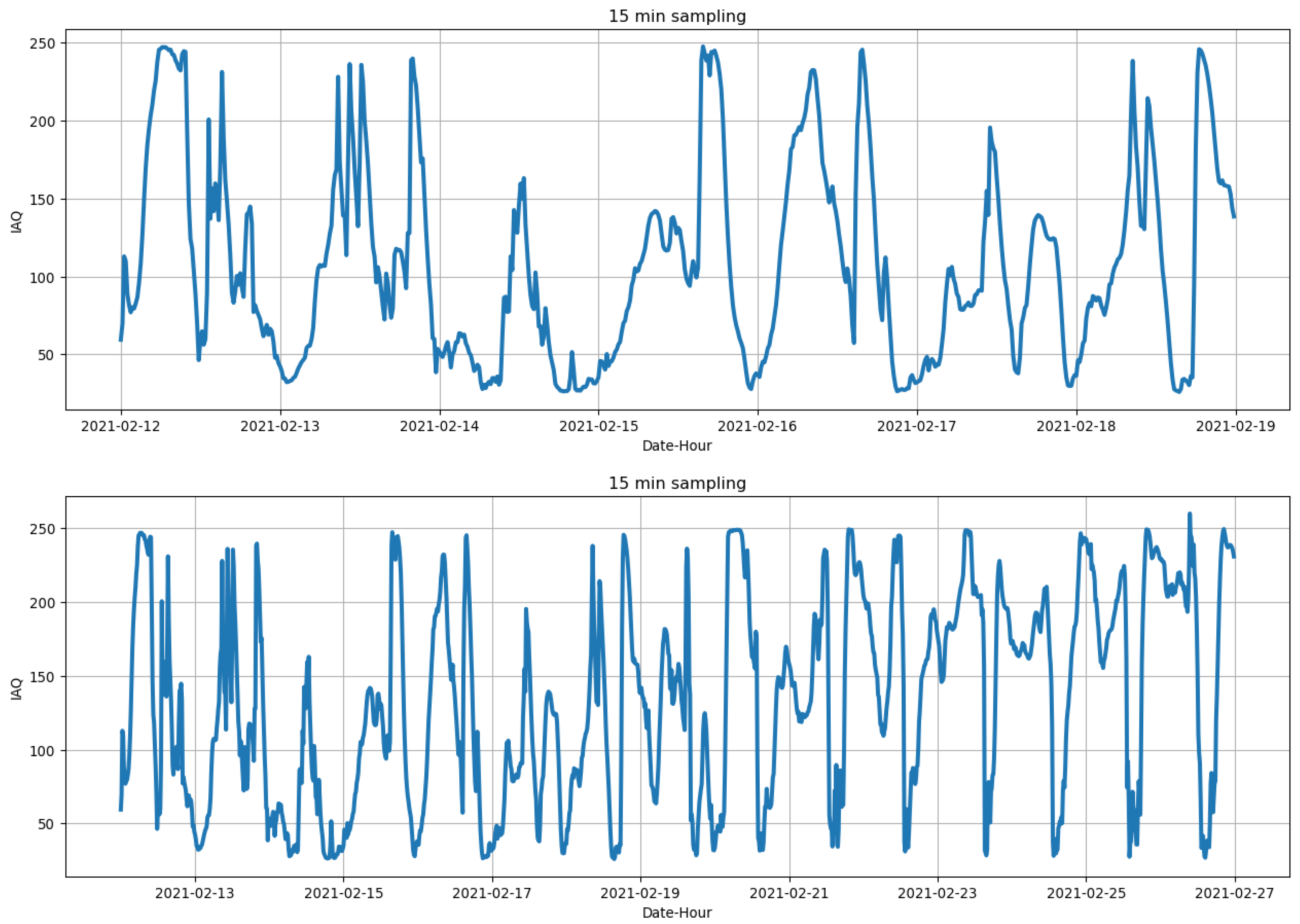
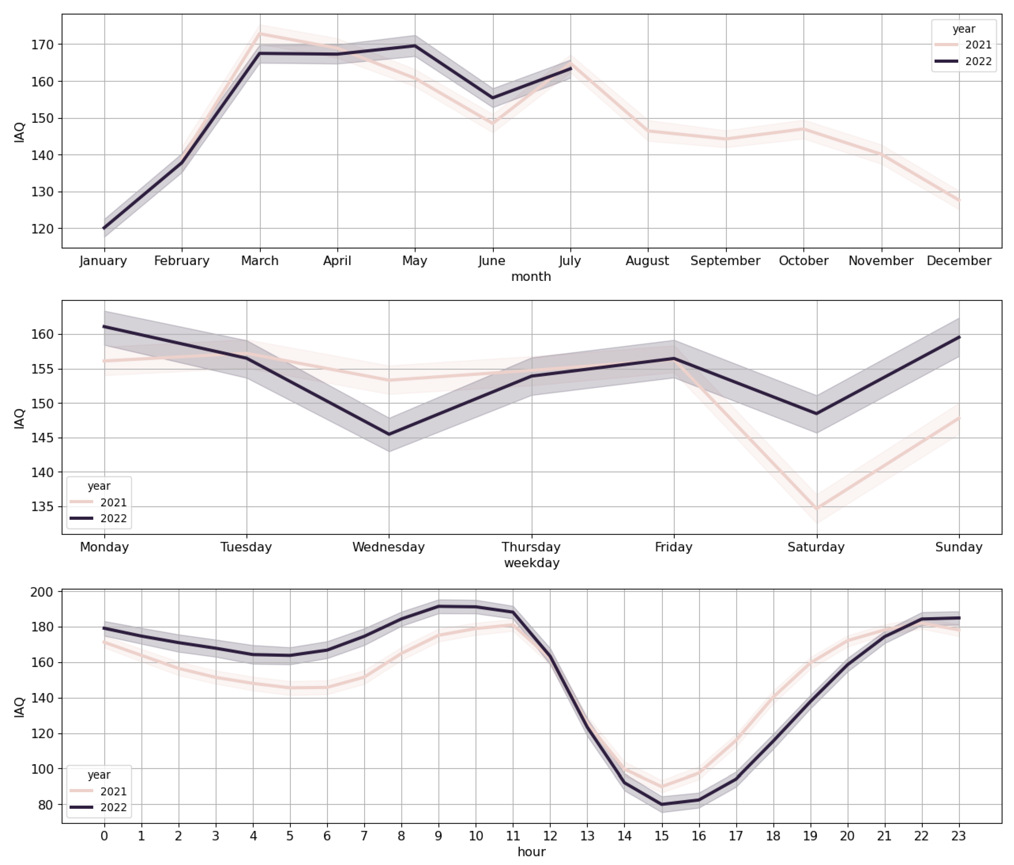
3.4. Exploratory Data Analysis

This section presents visualizations, distributions, and findings for the IAQ variable as well as its auto-correlation and partial auto-correlation. In addition, it presents a cross-correlation analysis between the IAQ and the independent variables. For efficiency, we used a sampling rate of 15 min (i.e., a subsampling of the data collected every 3 s) for this exploratory data analysis.

Figure 2 shows the time series for the IAQ for one and two weeks. As shown in the 2-week time series of Figure 2, there is a slight seasonal pattern that repeats daily. In addition, Figure 3 shows the distribution of the IAQ target variable as a function of time. Concretely, we can see its mean and standard deviation as a function of the month, day of the week, and hour. Looking at the monthly distributions, we can see a trend that seems to repeat yearly (based on the current records), growing from 120 in January to 170 during March, April, and May, and then smoothly decreasing to 130 in December. This increase in the IAQ coincides with the highest temperatures in Mexico City through the year. Also, the decreases in June and December–January can be explained by the summer and winter holiday seasons for schools, which are accompanied by a considerable decrease in the number of vehicles circulating throughout the city.

Figure 2. Time series for the IAQ: One and two weeks provided for showing details and more general behavior, respectively. Sampled every 15 min.

Figure 3. Mean and standard deviation of the time series for the IAQ: Distributions per month, day of the week, and hour.

Interpreting the IAQ on a daily basis is less straight forward; see Figure 3. The peaks of Monday, and perhaps those of Sunday, might be due to the fact that many people drive away from the city during weekends and come back either on Sunday afternoon and evening or early morning on Monday, which might also explain the valleys on Saturdays. However, the reason for the relative drop on Wednesdays is rather unclear. In addition, when looking at the distribution per hour (Figure 3), we can observe an expected peak between 8:00 and 10:00 h. However, its relative increase is only marginal with respect to the majority of the night hours, which is an unexpected observation. The valley between 14:00 and 17:00 h coincides with common lunch hours in Mexico.

Going further in the analysis, we conducted an augmented Dickey–Fuller test, which indicates that the time series of IAQ is stationary, i.e., the test rejects the null hypothesis stating that there exists a unit root in the time series and that it is non-stationary (p-value < 0.01).

Figure 4 shows the auto-correlation and the partial auto-correlation of the IAQ for its first 120 past records, also known as lags. As we can see, the IAQ exhibits high auto-correlation within the first 15 lags, i.e., up to 4 h of history. Additionally, the partial auto-correlation analysis shows that there is a strong independent correlation with the two closest historical records but not further. Therefore, the auto-correlation and partial auto-correlation analyses suggest that it may be possible to make use of traditional linear models, e.g., ARIMA, to forecast the IAQ based on lagged observations of itself. However, our present work (as indicated in Section 3.3) does not use lagged observations of the IAQ to forecast it. Hence, the deployment of our deep learning models integrated into an electronic forecasting device can be performed using sensors reporting only concentration levels of pollutants, without requiring a sensor reporting an indoor air quality index.

Figure 4. Auto-correlation and partial auto-correlation plots for the first 120 lags, sampled every 15 min from the time series for the IAQ.

Figure 5 shows the cross-correlation between the IAQ target variable and the independent variables. In this context, the cross-correlation analysis indicates to what extent there are temporal (linear) relationships between the concentration levels of each pollutant and the IAQ, i.e., what pollutant may have contributed the most to the IAQ, although it should be noted that cross-correlation per se does not imply causation.

Figure 5. Cross-correlation and lagged cross-correlation between the IAQ target variable and the independent variables up to 120 lags.

In this regard, the IAQ is, to some extent, cross-correlated with indoor variables (such as temperature, pressure, and relative humidity) and outdoor pollution indicators (such as NO, ${\mathrm{NO}}_2$, ${\mathrm{PM}}_{10}$, ${\mathrm{PM}}_{2.5}$, and ${\mathrm{SO}}_2$) as shown in Figure 5. Nevertheless, those cross-correlations may be regarded as relatively weak, with values below 0.1 for the different pollutants. Moreover, the analysis on lagged records of the independent variables is consistent with these cross-correlations up to 120 lagged observations. That is to say that the correlation between the target variable and the pollutants is consistent for up to 30 h. Despite the relatively negligible linear cross-correlations between the target variable and the independent variables, our experimental results show that it is possible to forecast the IAQ using non-linear models; concretely, deep learning models (see Section 4).

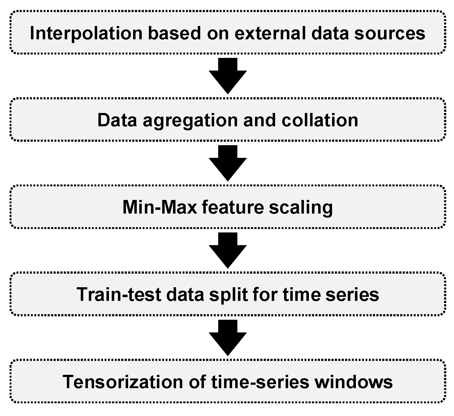
3.5. Data Curation and Preprocessing

The exploratory data analysis (Section 3.4) supported the data curation and preprocessing (see Figure 6).

Figure 6. Implemented data pipeline for preprocessing the time-series data.

The reporting rate of the external data sources (SINAICA and OpenWeather) is once every hour. Therefore, a linear interpolation was needed to match the 3 s reporting interval of the Bosch BME680 sensor. In this interpolation, we added Gaussian noise to avoid overfitting our models.

All three data sources (sensor, SINAICA, and OpenWeather) were joined based on the local time to generate a single table. This local time key was synchronized using the network time protocol, which encodes the official time in Mexico City. This process created a single multi-sensor signal, i.e., a time series of multiple channels. Since our data set had variables with different ranges, we scaled them down into a range between 0 and 1 using the well-known MinMax scaler.

The sampling rate of the sensor, of 3 s, generated a large number of records, which is computationally intensive and beyond our budget. Therefore, we resampled the data set considering three different sampling rates: 5, 10, and 15 min. For each sampling rate, we used the arithmetic mean as the value of the observation.

It should be noted that we split the data set into train and test sets, using 70% and 30% of the records, respectively, which is a common practice in the field.

3.6. Models

Given the nature of the forecasting problem, we relied on deep learning models that are of the following form:

$$y\left(t\right)=f\left(\mathbf{x}(t-1),\mathbf{x}(t-2),\dots ,\mathbf{x}(t-N);\Omega \right),$$

(1)

where $y\left(t\right)$ represents the scalar target value to be predicted (IAQ) at time t; $f(·)$ represents the forecasting function (i.e., a deep neural network in our present work); $\mathbf{x}\left(t\right)$ corresponds to a vector containing the 14 input variables used as predictors (listed in Section 3.3) at time t; N is a hyperparameter that controls the number of past records that are considered as predictors; and $\Omega$ refers to a set of parameters of the model, which are learned from the training data during the training process.

Four neural network base architectures were selected to compare their forecasting performance:

• Dense neural networks (DNNs), also commonly referred to as fully connected neural networks or multilayer perceptrons.
• Long short-term memory (LSTM) neural networks.
• One-dimension convolutional neural networks (CNNs).
• A combination of the above base architectures to exploit their advantages.

The above architectures were selected because they are commonly used to create forecasting models; see, for instance, [29,44]. It should be noted that we explored the performance of these neural network architectures using different levels of depth (see Section 4). Also notice that in the machine learning jargon, a model is defined as the combination of a specific architecture, including its hyperparameters, and its corresponding set of parameters. Thus, our 133 models are the result of exploring the hyperparameter space for these four base architectures, and learning their respective sets of parameters.

3.7. Training-Phase Implementation

We built models using 153 days of training data (roughly five months of data) and models using 372 days of training data (over a year of data). We decided to define these two scenarios to explore whether there is an impact on forecasting performance from using different amounts of training data and possible seasonal patterns.

We used a sequence length of seven days of history as input for all models. The data were treated according to the above descriptions, and then they were submitted to a Google Vertex AI container for hyperparameter optimization and model training. For each deep learning architecture, the hyperparameters tuned were stride in the range (1, 3), sampling rate in the range (1, 2), historic windows in minutes in the set {2, 5, 10, 15}, and batch size in the set {128, 256, 512}. We also fixed the number of neurons to 64 in the LSTM layer of our models. In the case of CNNs, we used 16 filters of size 3, meaning that the kernels were allowed to see only 3 historic samples at a time. All hidden layers for the DNN and CNN models used the ReLU non-linear activation, while the LSTM used its default sigmoid and hyperbolic tangent functions. Also, the CNN models made use of padding and MaxPooling functions. For the optimization of the deep learning models, Adam [45] and stochastic gradient descent [46] were used. We minimized the mean square error (MSE) loss function, which is a common practice in air pollution forecasting [47].

4. Results and Discussion

The descriptions of the models reported in Table 1 are as follows:

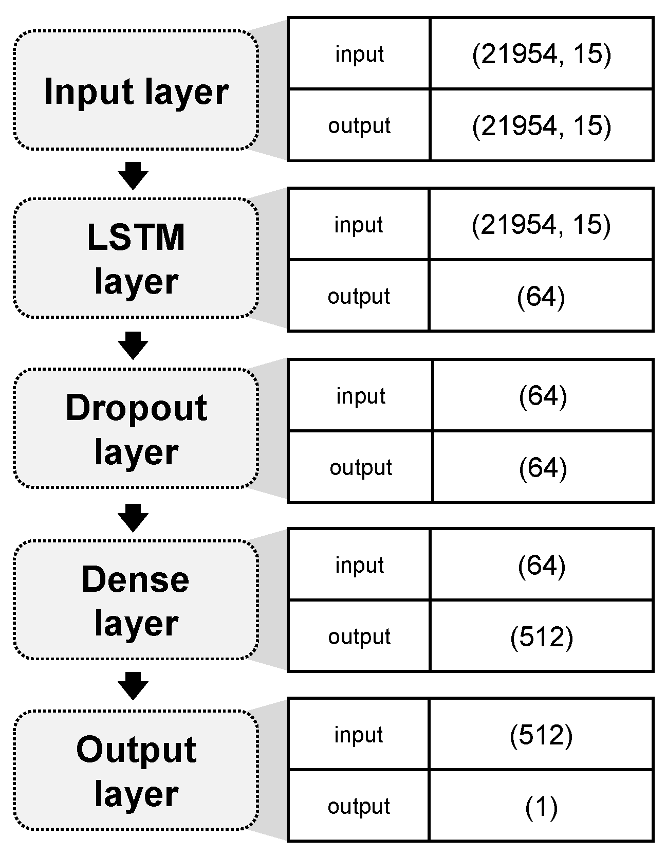
• LSTM02 is a 2-layer model based on LSTM with a dropout layer (see Figure 7).
  

  Figure 7. Architecture of the top-performing model: LSTM02.
• LSTM05 is a 5-layer model based on LSTM.
• DEEP17 is a 17-layer deep learning model combining LSTM, MLP, and CNNs.
• CONV02 is a 2-layer model based on 1-dimension CNNs.
• DNN03 is a 3-layer dense neural network, i.e., a fully connected or multilayer perceptron model.

Table 1. Top-performing models ordered by MSE and MAE.

Model Type	Layers	Params	Stride	Sampling Rate	Training Data	MSE	MAE
LSTM02	2	54,273	1	2	<1 Year	0.0179	0.1038
LSTM05	5	185,345	2	2	>1 Year	0.0190	0.1162
DEEP17	17	169,795	1	2	>1 Year	0.0193	0.1205
LSTM02	2	54,273	2	2	>1 Year	0.0197	0.1219
LSTM02	2	54,273	1	2	>1 Year	0.0197	0.1227
LSTM05	5	185,345	1	2	>1 Year	0.0198	0.1218
DEEP17	17	169,795	2	2	>1 Year	0.0202	0.1243
LSTM05	5	185,345	2	2	>1 Year	0.0203	0.1219
CONV02	2	706	2	2	<1 Year	0.0203	0.1303
DNN03	3	8705	2	2	<1 Year	0.0204	0.1268
DT	–	–	1	2	<1 Year	0.0293	0.1418
DT	–	–	1	2	>1 Year	0.0208	0.1239
RF	–	–	1	2	<1 Year	0.0260	0.1358
RF	–	–	1	2	>1 Year	0.0177	0.1130

Table 1. Top-performing models ordered by MSE and MAE.

Model Type	Layers	Params	Stride	Sampling Rate	Training Data	MSE	MAE
LSTM02	2	54,273	1	2	<1 Year	0.0179	0.1038
LSTM05	5	185,345	2	2	>1 Year	0.0190	0.1162
DEEP17	17	169,795	1	2	>1 Year	0.0193	0.1205
LSTM02	2	54,273	2	2	>1 Year	0.0197	0.1219
LSTM02	2	54,273	1	2	>1 Year	0.0197	0.1227
LSTM05	5	185,345	1	2	>1 Year	0.0198	0.1218
DEEP17	17	169,795	2	2	>1 Year	0.0202	0.1243
LSTM05	5	185,345	2	2	>1 Year	0.0203	0.1219
CONV02	2	706	2	2	<1 Year	0.0203	0.1303
DNN03	3	8705	2	2	<1 Year	0.0204	0.1268
DT	–	–	1	2	<1 Year	0.0293	0.1418
DT	–	–	1	2	>1 Year	0.0208	0.1239
RF	–	–	1	2	<1 Year	0.0260	0.1358
RF	–	–	1	2	>1 Year	0.0177	0.1130

Table 1 does not show the hyperparameters for the decision tree and random forest models, as they are not directly comparable against those of deep learning architectures. However, a grid search over their hyperparameter spaces resulted in the following models.

• DT is a decision tree with a Poisson split criterion, a maximum depth of three levels, and as many features as the square root of the initial number of input variables.
• RF is a random forest model with 30 trees, a maximum depth of three levels, and as many features as the square root of the initial number of input variables.

From Table 1, we can see that the best-performing models are LSTM-based architectures. More precisely, 6 models out of these 14 are LSTM-based architectures, including the best-performing model: LSTM02, whose architecture is presented in Figure 7. This behavior was expected in comparison with the use of pure dense neural network models, as the recurrence operator of the LSTM is designed to accumulate historic patterns, and to incorporate or eliminate past information as it sees fit. Therefore, these results confirm previous observations regarding the fact that LSTMs are more robust for historic data than dense models.

We also expected LSTM-based models to outperform CNNs, as we defined relatively small convolutional kernels to maintain efficiency in terms of model size, i.e., the use of larger convolutional kernels also increases the number of parameters of these models. The results shown in Table 1 confirm that this is indeed the case.

Nonetheless, it was rather surprising to notice that, in general, the DEEP17 models were also outperformed by the best LSTM-based model. This is surprising because DEEP17 models combine LSTM, 1D convolutions, and fully connected layers. From our analysis, we can infer that their limited performance on the test set is evidence of over-parametrization. That being said, when comparing the third and fifth rows of Table 1, which correspond to the same configuration of data in terms of length and sampling rate, we can observe that the model DEEP17 achieved slightly better performance than LSTM02, suggesting that for long periods of data, it might be better to accompany the LSTM with subsequent processing steps provided by convolutions and fully connected units. Nevertheless, notice that DEEP17 consists of roughly 3.15 times the number of parameters of LSTM02, making it more costly in computational terms. Furthermore, the decision tree models remained behind all other models.

As reported in Table 1, many of the best-performing models are shallow, i.e., with only a few layers. In fact, the models with the best performance have around 50,000 parameters. Figure 8 shows the performance of the models that we evaluated with respect to their number of parameters. As we can observe, larger models tend to overfit, and thus result in a higher MSE on the test set. Additionally, Table 1 also shows that neither the stride nor the historic length of the data seem to have a clear effect on the performance of these models.

Figure 8. Deep learning models for indoor air quality forecasting: performance vs. size.

Finally, from Table 1 we can observe that random forest models are capable of obtaining an MSE of 0.0177, which is slightly lower than that obtained with LSTM02. However, the performance of the random forest model is obtained using all 17 months of data, whereas the LSTM achieved its lowest error rate with only 5 months of data, making it a more effective solution.

Overall, we can list our findings as follows. First, the best-performing model is the LSTM for data sets of short historical length, whereas for longer historical records, the combination of LSTM, 1D convolutions, and fully connected layers achieves slightly higher performance. Second, shallow models with around 50,000 parameters have enough capacity to achieve the best forecasting performance, while larger and deeper models correspond to over-parametrized options that end up in overfitting. Third, neither the variations in the stride nor the sampling rate have an impact on the performance of these models. And fourth, random forest models are also promising alternatives, but they require data sets of long historical context, as opposed to the potential shown by the LSTM model using only five months of data.

In contrast to adopting a classification approach as in [34], our empirical results show that it is feasible to forecast an indoor air quality index based on concentration levels of pollutants. In addition, other works, such as [36,37,38,39], built independent models for each pollutant with the aim of forecasting indoor air quality; however, our results provide evidence for the feasibility of directly forecasting an indoor air quality index. Moreover, unlike the work by Abdullah et al. [32] that made use of a genetic algorithm for updating weights of an artificial neural network for forecasting concentration levels of pollutants, our results show that optimizing our deep learning models using the back-propagation algorithm yielded a relatively negligible MSE and MAE.

5. Conclusions

In this work, we designed and implemented an indoor air quality forecasting system composed of a second-generation Raspberry Pi and an air quality sensor. The air quality forecasting is supported by a deep learning model, in particular, an LSTM-based model with an MSE of 0.0179 and an MAE of 0.1038. To find the best forecasting model, we conducted extensive experimentation involving different deep learning architectures and exploring a myriad of hyperparameters. The models were trained with data from over 17 months of (i) indoor air quality records collected via our proposed system, (ii) publicly available air pollution records provided by a Mexican government agency, and (iii) weather data provided by OpenWeather corresponding to Mexico City. Among the 133 deep learning models evaluated, in general, LSTM-based models outperformed CNNs, DNNs, and hybrid models.

This work contributes to the state of the art in forecasting indoor air quality by implementing a forecasting system capable of predicting an IAQ (unlike other research efforts forecasting concentration levels of pollutants; see Table A1). In addition, this work also contributes a curated data set of 17 months of indoor and outdoor air quality records from three different data sources, which has been made available for research purposes.

Based on our experimental results and when forecasting an IAQ in relatively large cities, we recommend using LSTM-based architectures over CNNs, DNNs, hybrid architectures, decision trees, and random forests due to their capacity to accumulate historic patterns while incorporating or eliminating past information as they see fit. From a technical point view, when conducting extensive experimentation to build, combine, and evaluate myriad deep learning models (such as in our present work), we recommend using automated cloud resource orchestration and parallel hyperparameter tuning on cloud environments such as Google Vertex AI.

We would like to highlight that our results can be applied in sustainable smart devices, such as air purifiers or automatic air vents that incorporate forecasting capabilities (as described in this article) in order to be activated when needed, avoiding unnecessary energy consumption and its associated costs.

Since our present work has provided empirical evidence for the feasibility of forecasting an indoor air quality index based on indoor and outdoor concentration levels of common pollutants, our future work will be focused on deploying multiple sensors to collect data related to indoor air quality at different locations in Mexico City and under different circumstances. For instance, deploying indoor air quality sensors in houses and apartment buildings with different ventilation systems. With our proposed experimental methodology and a considerably large data set, our future work will also focus on training new deep learning models. Also, we will explore other machine learning techniques and traditional forecasting methods.

References

- Tran, H.M.; Tsai, F.J.; Lee, Y.L.; Chang, J.H.; Chang, L.T.; Chang, T.Y.; Chung, K.F.; Kuo, H.P.; Lee, K.Y.; Chuang, K.J.; et al. The impact of air pollution on respiratory diseases in an era of climate change: A review of the current evidence. Sci. Total Environ. 2023, 898, 166340. [Google Scholar] [CrossRef] [PubMed]
- Liao, M.; Braunstein, Z.; Rao, X. Sex differences in particulate air pollution-related cardiovascular diseases: A review of human and animal evidence. Sci. Total Environ. 2023, 884, 163803. [Google Scholar] [CrossRef] [PubMed]
- Cole-Hunter, T.; Zhang, J.; So, R.; Samoli, E.; Liu, S.; Chen, J.; Strak, M.; Wolf, K.; Weinmayr, G.; Rodopolou, S.; et al. Long-term air pollution exposure and Parkinson’s disease mortality in a large pooled European cohort: An ELAPSE study. Environ. Int. 2023, 171, 107667. [Google Scholar] [CrossRef] [PubMed]
- Tian, F.; Qi, J.; Qian, Z.; Li, H.; Wang, L.; Wang, C.; Geiger, S.D.; McMillin, S.E.; Yin, P.; Lin, H.; et al. Differentiating the effects of air pollution on daily mortality counts and years of life lost in six Chinese megacities. Sci. Total Environ. 2022, 827, 154037. [Google Scholar] [CrossRef]
- Liu, Y.; Tong, D.; Cheng, J.; Davis, S.J.; Yu, S.; Yarlagadda, B.; Clarke, L.E.; Brauer, M.; Cohen, A.J.; Kan, H.; et al. Role of climate goals and clean-air policies on reducing future air pollution deaths in China: A modelling study. Lancet Planet. Health 2022, 6, e92–e99. [Google Scholar] [CrossRef]
- Tsai, S.S.; Chen, C.C.; Yang, C.Y. The impacts of reduction in ambient fine particulate (PM2. 5) air pollution on life expectancy in Taiwan. J. Toxicol. Environ. Health Part A 2022, 85, 913–920. [Google Scholar] [CrossRef] [PubMed]
- Shetty, S.S.; Deepthi, D.; Harshitha, S.; Sonkusare, S.; Naik, P.B.; Suchetha, K.N.; Madhyastha, H. Environmental pollutants and their effects on human health. Heliyon 2023, 9, e19496. [Google Scholar] [CrossRef] [PubMed]
- Huang, W.; Li, T.; Liu, J.; Xie, P.; Du, S.; Teng, F. An overview of air quality analysis by big data techniques: Monitoring, forecasting, and traceability. Inf. Fusion 2021, 75, 28–40. [Google Scholar] [CrossRef]
- Saini, J.; Dutta, M.; Marques, G. A comprehensive review on indoor air quality monitoring systems for enhanced public health. Sustain. Environ. Res. 2020, 30, 6. [Google Scholar] [CrossRef]
- Kumar, P.; Kumar, P. A critical evaluation of air quality index models (1960–2021). Environ. Monit. Assess. 2022, 194, 324. [Google Scholar] [CrossRef]
- AirNow. Air Quality Index (AQI) Basics. 2024. Available online: https://www.airnow.gov/aqi/aqi-basics/ (accessed on 1 November 2024).
- Bosch. Bosch BME680 Datasheet. 2024. Available online: https://www.bosch-sensortec.com/media/boschsensortec/downloads/datasheets/bst-bme680-ds001.pdf (accessed on 1 November 2024).
- Gunatilaka, D.; Sanbundit, P.; Puengchim, S.; Boontham, C. AiRadar: A Sensing Platform for Indoor Air Quality Monitoring. In Proceedings of the 2022 19th International Joint Conference on Computer Science and Software Engineering, Bangkok, Thailand, 8–10 June 2022; pp. 1–6. [Google Scholar] [CrossRef]
- Streuber, D.; Park, Y.M.; Sousan, S. Laboratory and Field Evaluations of the GeoAir2 Air Quality Monitor for Use in Indoor Environments. Aerosol Air Qual. Res. 2022, 22, 220119. [Google Scholar] [CrossRef] [PubMed]
- Markozannes, G.; Pantavou, K.; Rizos, E.C.; Sindosi, O.A.; Tagkas, C.; Seyfried, M.; Saldanha, I.J.; Hatzianastassiou, N.; Nikolopoulos, G.K.; Ntzani, E. Outdoor air quality and human health: An overview of reviews of observational studies. Environ. Pollut. 2022, 306, 119309. [Google Scholar] [CrossRef]
- Chen, J.; Yuan, C.; Dong, S.; Feng, J.; Wang, H. A novel spatiotemporal multigraph convolutional network for air pollution prediction. Appl. Intell. 2023, 53, 18319–18332. [Google Scholar] [CrossRef]
- Ge, L.; Wu, K.; Zeng, Y.; Chang, F.; Wang, Y.; Li, S. Multi-scale spatiotemporal graph convolution network for air quality prediction. Appl. Intell. 2021, 51, 3491–3505. [Google Scholar] [CrossRef]
- Mannan, M.; Al-Ghamdi, S.G. Indoor air quality in buildings: A comprehensive review on the factors influencing air pollution in residential and commercial structure. Int. J. Environ. Res. Public Health 2021, 18, 3276. [Google Scholar] [CrossRef] [PubMed]
- Liu, F.; Yan, L.; Meng, X.; Zhang, C. A review on indoor green plants employed to improve indoor environment. J. Build. Eng. 2022, 53, 104542. [Google Scholar] [CrossRef]
- Shaw, D.; Carslaw, N. INCHEM-Py: An open source Python box model for indoor air chemistry. J. Open Source Softw. 2021, 6, 3224. [Google Scholar] [CrossRef]
- Liu, N.; Liu, W.; Deng, F.; Liu, Y.; Gao, X.; Fang, L.; Chen, Z.; Tang, H.; Hong, S.; Pan, M.; et al. The burden of disease attributable to indoor air pollutants in China from 2000 to 2017. Lancet Planet. Health 2023, 7, e900–e911. [Google Scholar] [CrossRef] [PubMed]
- Tian, S.; Wang, L.; Liu, Q.; Luo, L.; Qian, C.; Wang, B.; Liu, Y. Associations between Indoor and Outdoor Size-Resolved Particulate Matter in Urban Beijing: Chemical Compositions, Sources, and Health Risks. Atmosphere 2024, 15, 721. [Google Scholar] [CrossRef]
- Salthammer, T.; Zhao, J.; Schieweck, A.; Uhde, E.; Hussein, T.; Antretter, F.; Künzel, H.; Pazold, M.; Radon, J.; Birmili, W. A holistic modeling framework for estimating the influence of climate change on indoor air quality. Indoor Air 2022, 32, e13039. [Google Scholar] [CrossRef] [PubMed]
- Wu, H.W.; Kumar, P.; Cao, S.J. Evaluation of ventilation and indoor air quality inside bedrooms of an elderly care centre. Energy Build. 2024, 313, 114245. [Google Scholar] [CrossRef]
- Vasile, V.; Catalina, T.; Dima, A.; Ion, M. Pollution Levels in Indoor School Environment—Case Studies. Atmosphere 2024, 15, 399. [Google Scholar] [CrossRef]
- Morawska, L.; Allen, J.; Bahnfleth, W.; Bennett, B.; Bluyssen, P.M.; Boerstra, A.; Buonanno, G.; Cao, J.; Dancer, S.J.; Floto, A.; et al. Mandating indoor air quality for public buildings. Science 2024, 383, 1418–1420. [Google Scholar] [CrossRef]
- Mohammed, M.A.; Ahmed, L.A. Forecasting wind speed using the proposed wavelet neural network. Discret. Dyn. Nat. Soc. 2023, 2023, 9940038. [Google Scholar] [CrossRef]
- Kolambe, M.; Arora, S. Forecasting the future: A comprehensive review of time series prediction techniques. J. Electr. Syst. 2024, 20, 575–586. [Google Scholar]
- Zhang, L.; Dou, H.; Zhang, K.; Huang, R.; Lin, X.; Wu, S.; Zhang, R.; Zhang, C.; Zheng, S. CNN-LSTM Model Optimized by Bayesian Optimization for Predicting Single-Well Production in Water Flooding Reservoir. Geofluids 2023, 2023, 5467956. [Google Scholar] [CrossRef]
- SINAICA. Sistema Nacional de Información de la Calidad del Aire del Gobierno Federal México. 2024. Available online: https://sinaica.inecc.gob.mx/ (accessed on 1 November 2024).
- OpenWeather. History Bulk Weather Data. 2024. Available online: https://openweathermap.org/history-bulk (accessed on 1 November 2024).
- Abdullah, A.; Usmani, R.S.A.; Pillai, T.; Marjani, M.; Abaker, I.; Hashem, I. An Optimized Artificial Neural Network Model using Genetic Algorithm for Prediction of Traffic Emission Concentrations. Int. J. Adv. Comput. Sci. Appl. 2021, 12, 794–803. [Google Scholar] [CrossRef]
- Cakir, S.; Sita, M. Evaluating the performance of ANN in predicting the concentrations of ambient air pollutants in Nicosia. Atmos. Pollut. Res. 2020, 11, 2327–2334. [Google Scholar] [CrossRef]
- Kumbhar, V.S.; Sohi, S.S.; Jayaram, V.; Sreelekshmy, P.G.; Shukla, S.K.; Abhilash, K.S. Hybrid artificial neural network algorithm for air pollution estimation. Int. J. Health Sci. 2022, 6, 2094–2106. [Google Scholar] [CrossRef]
- Saad, S.; Andrew, A.; Shakaff, A.; Saad, A.; Kamarudin, A.; Zakaria, A. Classifying Sources Influencing Indoor Air Quality (IAQ) Using Artificial Neural Network (ANN). Sensors 2015, 15, 11665–11684. [Google Scholar] [CrossRef]
- Kapoor, N.R.; Kumar, A.; Kumar, A.; Kumar, A.; Mohammed, M.A.; Kumar, K.; Kadry, S.; Lim, S. Machine learning-based CO2 prediction for office room: A pilot study. Wirel. Commun. Mob. Comput. 2022, 1–16. [Google Scholar] [CrossRef]
- Ahn, J.; Shin, D.; Kim, K.; Yang, J. Indoor air quality analysis using deep learning with sensor data. Sensors 2017, 17, 2476. [Google Scholar] [CrossRef]
- Bakht, A.; Sharma, S.; Park, D.; Lee, H. Deep Learning-Based Indoor Air Quality Forecasting Framework for Indoor Subway Station Platforms. Toxics 2022, 10, 557. [Google Scholar] [CrossRef] [PubMed]
- Sharma, P.K.; Mondal, A.; Jaiswal, S.; Saha, M.; Nandi, S.; De, T.; Saha, S. IndoAirSense: A framework for indoor air quality estimation and forecasting. Atmos. Pollut. Res. 2021, 12, 10–22. [Google Scholar] [CrossRef]
- Pourkiaei, M.; Romain, A.C. Scoping review of indoor air quality indexes: Characterization and applications. J. Build. Eng. 2023, 75, 106703. [Google Scholar] [CrossRef]
- Rastogi, K.; Barthwal, A.; Lohani, D.; Acharya, D. An IoT-based discrete time Markov chain model for analysis and prediction of indoor air quality index. In Proceedings of the 2020 IEEE Sensors Applications Symposium, Kuala Lumpur, Malaysia, 9–11 March 2020; pp. 1–6. [Google Scholar] [CrossRef]
- Yue, Q.; Song, Y.; Zhang, M.; Zhang, X.; Wang, L. The impact of air pollution on employment location choice: Evidence from China’s migrant population. Environ. Impact Assess. Rev. 2024, 105, 107411. [Google Scholar] [CrossRef]
- Altamirano-Astorga, J.; Santiago-Castillejos, I.A.; Hernández-Martínez, L.; Roman-Rangel, E. Indoor Air Pollution Forecasting Using Deep Neural Networks. In Pattern Recognition; Vergara-Villegas, O.O., Cruz-Sánchez, V.G., Sossa-Azuela, J.H., Carrasco-Ochoa, J.A., Martínez-Trinidad, J.F., Olvera-López, J.A., Eds.; Springer: Cham, Switzerland, 2022; pp. 127–136. [Google Scholar] [CrossRef]
- Liu, J.; Huang, X.; Li, Q.; Chen, Z.; Liu, G.; Tai, Y. Hourly stepwise forecasting for solar irradiance using integrated hybrid models CNN-LSTM-MLP combined with error correction and VMD. Energy Convers. Manag. 2023, 280, 116804. [Google Scholar] [CrossRef]
- Li, H.; Rakhlin, A.; Jadbabaie, A. Convergence of Adam Under Relaxed Assumptions. In Advances in Neural Information Processing Systems, Proceedings of the NIPS ’23 37th International Conference on Neural Information Processing Systems, New Orleans, LA, USA, 10–16 December 2023; Oh, A., Naumann, T., Globerson, A., Saenko, K., Hardt, M., Levine, S., Eds.; Curran Associates, Inc.: Red Hook, NY, USA, 2023; Volume 36, pp. 52166–52196. [Google Scholar]
- Sclocchi, A.; Wyart, M. On the different regimes of stochastic gradient descent. Proc. Natl. Acad. Sci. USA 2024, 121, e2316301121. [Google Scholar] [CrossRef]
- Katzir, S. BreezoMeter’s Continuous Accuracy Testing for Reliable Air Quality Data. 2024. Available online: https://blog.breezometer.com/air-quality-accuracy-testing (accessed on 1 November 2024).
Disclaimer/Publisher’s Note: The statements, opinions and data contained in all publications are solely those of the individual author(s) and contributor(s) and not of MDPI and/or the editor(s). MDPI and/or the editor(s) disclaim responsibility for any injury to people or property resulting from any ideas, methods, instructions or products referred to in the content. |
© 2024 by the authors. Licensee MDPI, Basel, Switzerland. This article is an open access article distributed under the terms and conditions of the Creative Commons Attribution (CC BY) license (https://creativecommons.org/licenses/by/4.0/).
Share and Cite
Altamirano-Astorga, J.; Gutierrez-Garcia, J.O.; Roman-Rangel, E. Forecasting Indoor Air Quality in Mexico City Using Deep Learning Architectures. Atmosphere 2024, 15, 1529. https://doi.org/10.3390/atmos15121529
Altamirano-Astorga J, Gutierrez-Garcia JO, Roman-Rangel E. Forecasting Indoor Air Quality in Mexico City Using Deep Learning Architectures. Atmosphere. 2024; 15(12):1529. https://doi.org/10.3390/atmos15121529
Chicago/Turabian StyleAltamirano-Astorga, Jorge, J. Octavio Gutierrez-Garcia, and Edgar Roman-Rangel. 2024. "Forecasting Indoor Air Quality in Mexico City Using Deep Learning Architectures" Atmosphere 15, no. 12: 1529. https://doi.org/10.3390/atmos15121529
APA StyleAltamirano-Astorga, J., Gutierrez-Garcia, J. O., & Roman-Rangel, E. (2024). Forecasting Indoor Air Quality in Mexico City Using Deep Learning Architectures. Atmosphere, 15(12), 1529. https://doi.org/10.3390/atmos15121529