

Modeling of Precipitation Prediction Based on Causal Analysis and Machine Learning

Abstract
:1. Introduction
2. Information and Methodology
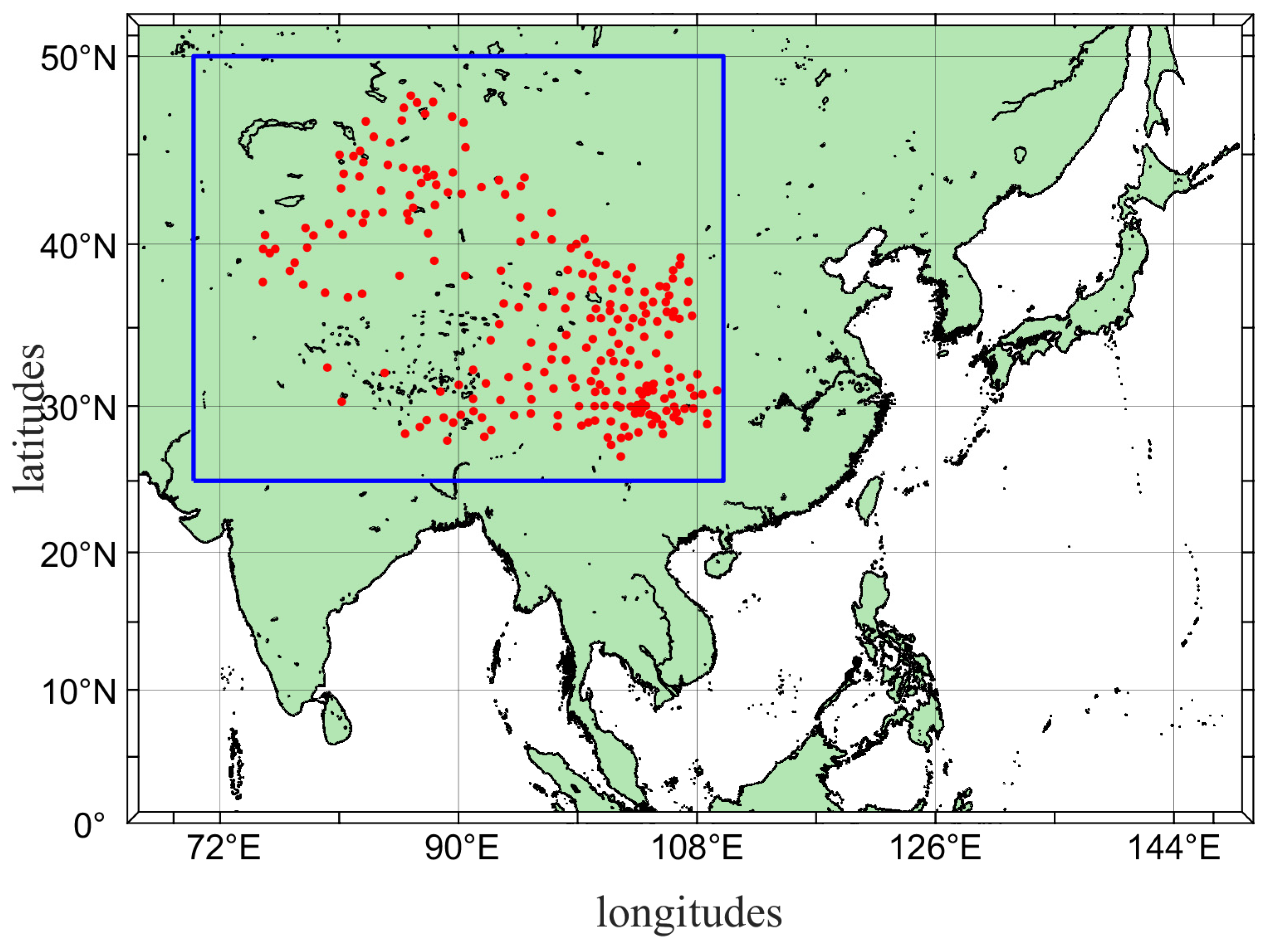
2.1. Data Sources
2.2. Assessment Methodology
2.3. Basic Theory of Information Flow
2.4. Machine Learning Methods
- (1)
- Back Propagation Neural Network
- (2)
- Random Forest
3. Experiments on Precipitation Prediction Based on Causal Analysis and Machine Learning Methods
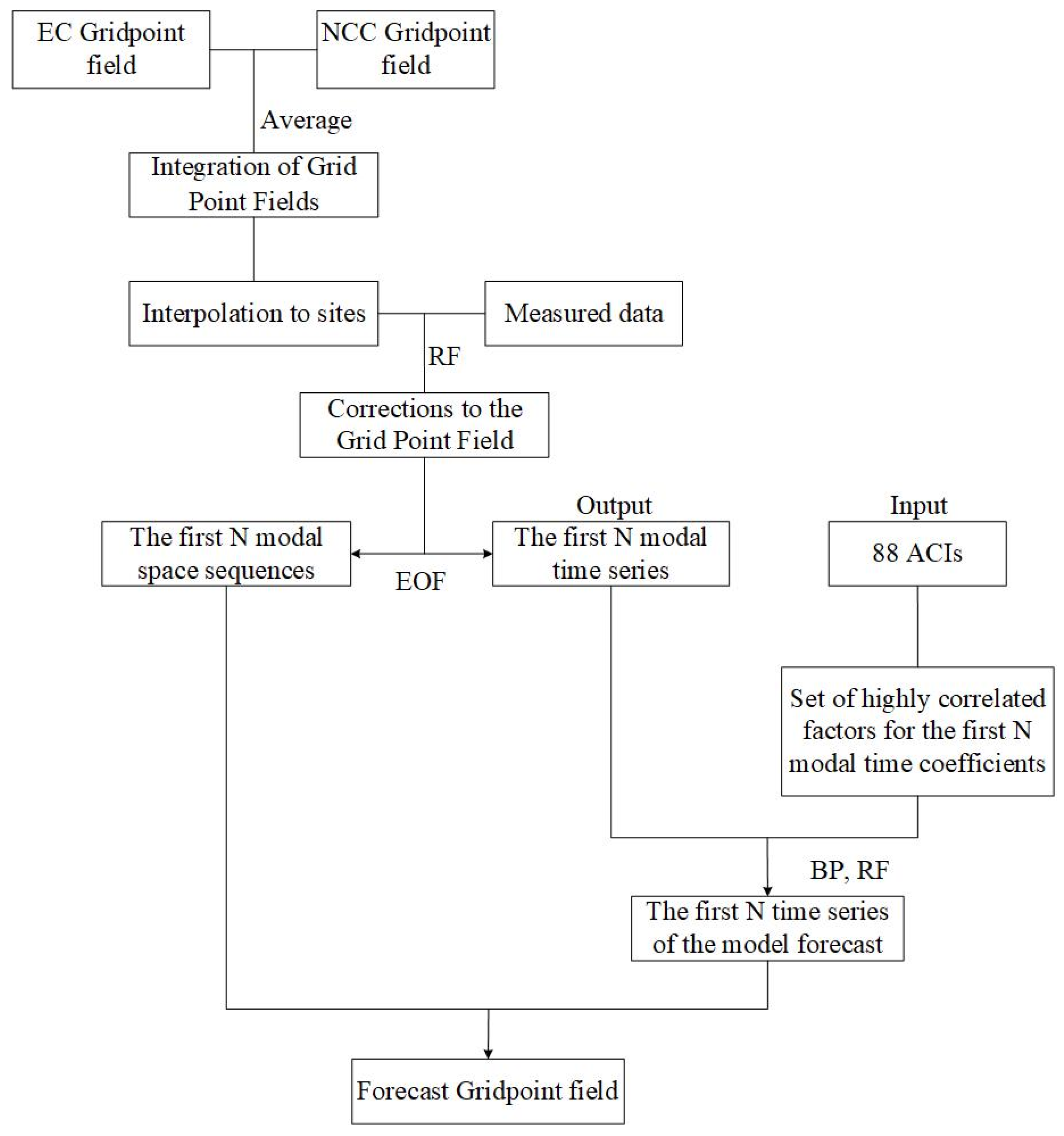
3.1. Technical Process for Modeling Precipitation Forecasts
- (1)
- Grid point field revision: This part takes the mean value of the EC and NCC grid point field to form a new grid point field, which is used to interpolate the grid point data into station data. After interpolation, the precipitation data of 240 stations are used as inputs, the measured data of 240 stations are used as outputs, and the RF algorithm is used to train the revised model. Based on the above model, the whole grid-point field is input to revise the original fusion grid-point field.
- (2)
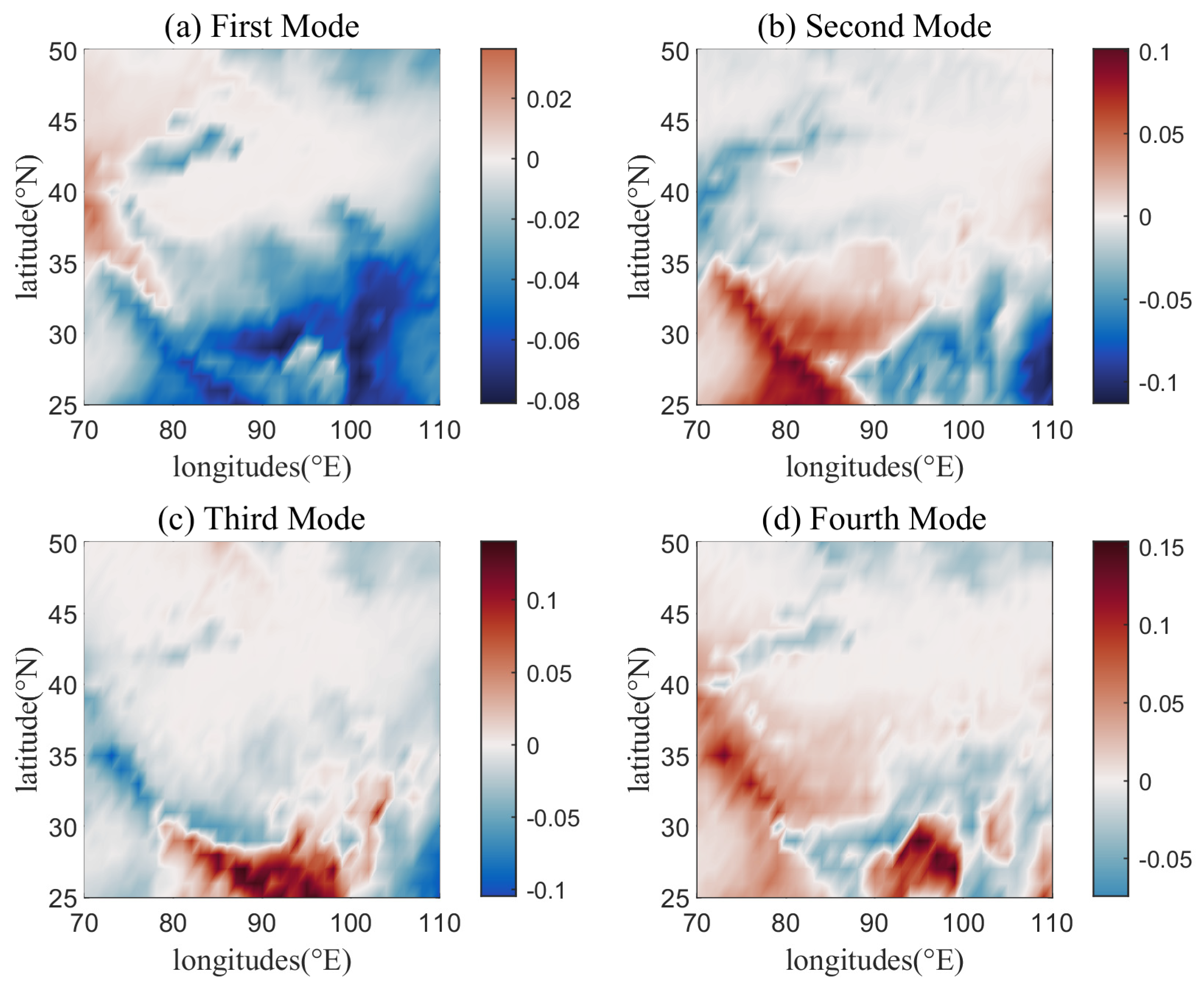
- Factor selection: The revised grid point field is stored in a standard format, where the first two dimensions are spatial, representing the latitude and longitude of the data, and the third dimension is temporal. Then, the revised grid point field is decomposed by the EOF into time series and spatial series, and the corresponding modes are selected according to the variance contribution of each mode. Each selected precipitation mode is subjected to information flow-based causal analysis using the set of atmospheric circulation indices to obtain a set of highly correlated factors for the time coefficients of the first N modes of precipitation.
- (3)
- Model building: This part sets the initial parameters according to the characteristics of THE BPNN and RF and combines the screened key factors with the decomposed time series for modeling.
- (4)
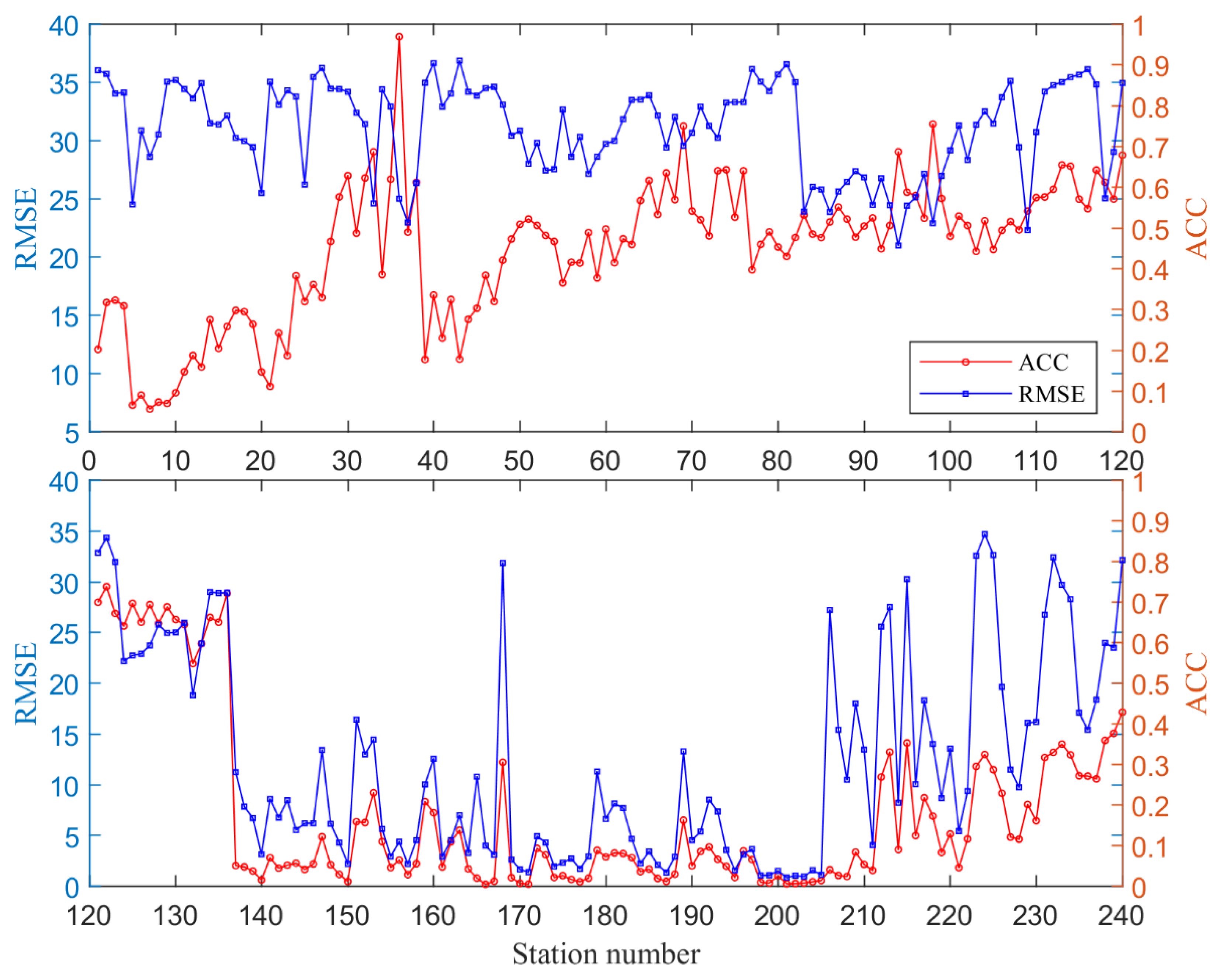
- Model prediction and effect test: The time coefficients of the model prediction and the spatial coefficients decomposed by the EOF are reduced to the prediction grid field. The prediction time limits are 1, 3, and 6 months, and the RMSE and ACC indicators evaluate the precipitation prediction ability of each station.
3.2. Precipitation Prediction Experiments
3.2.1. Selection of the Forecasting Factors
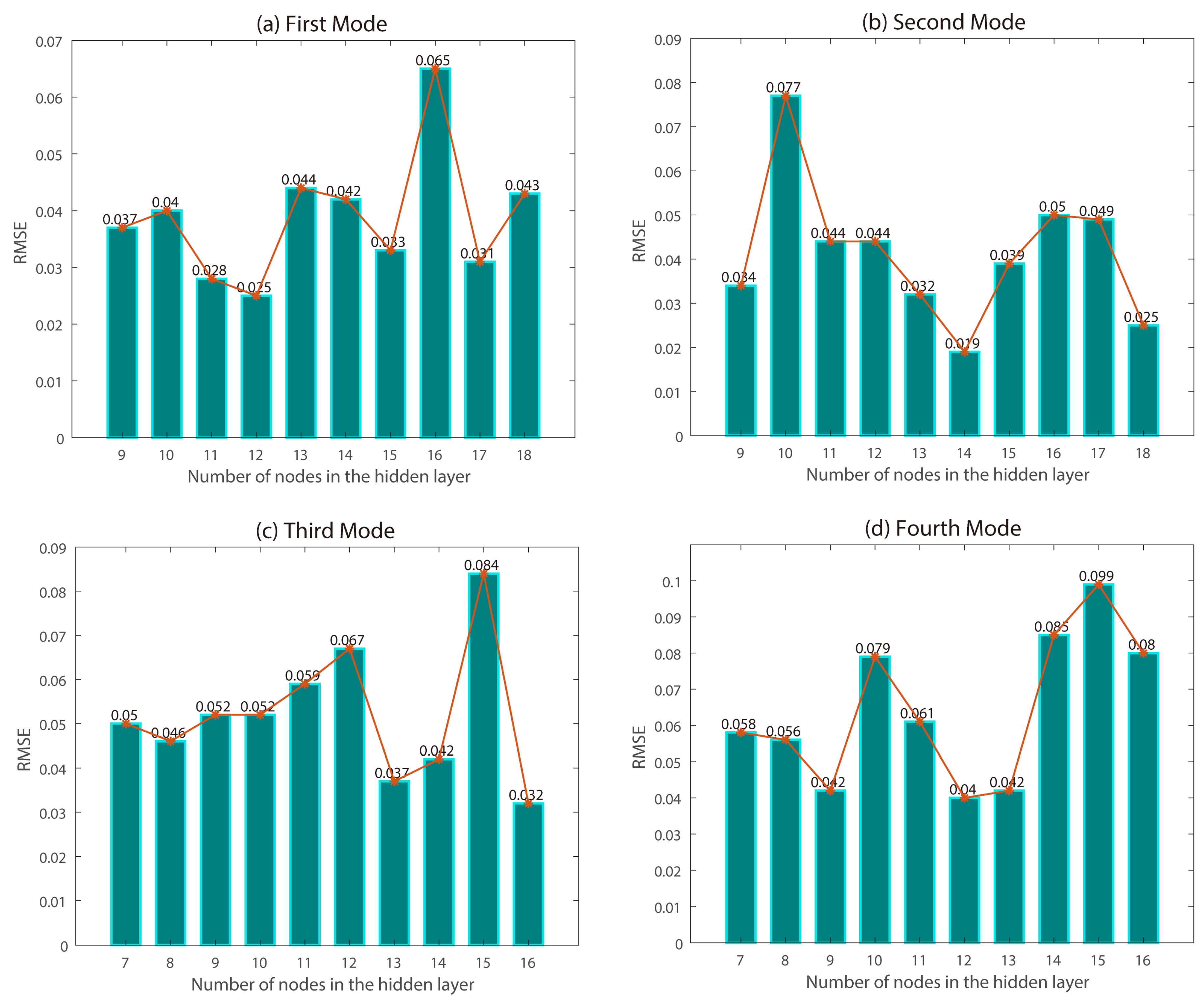
3.2.2. Machine Learning Model Parameter Settings
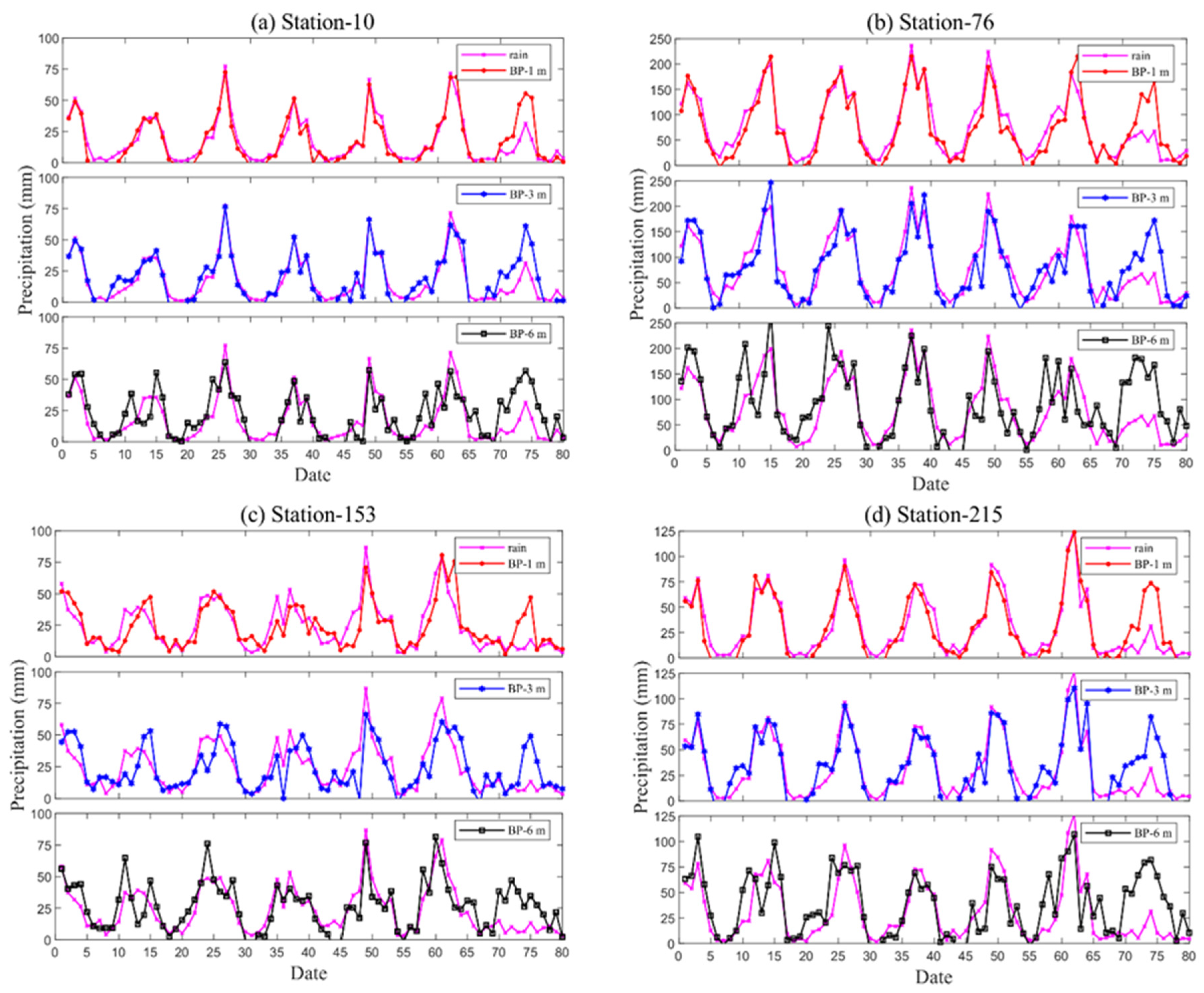
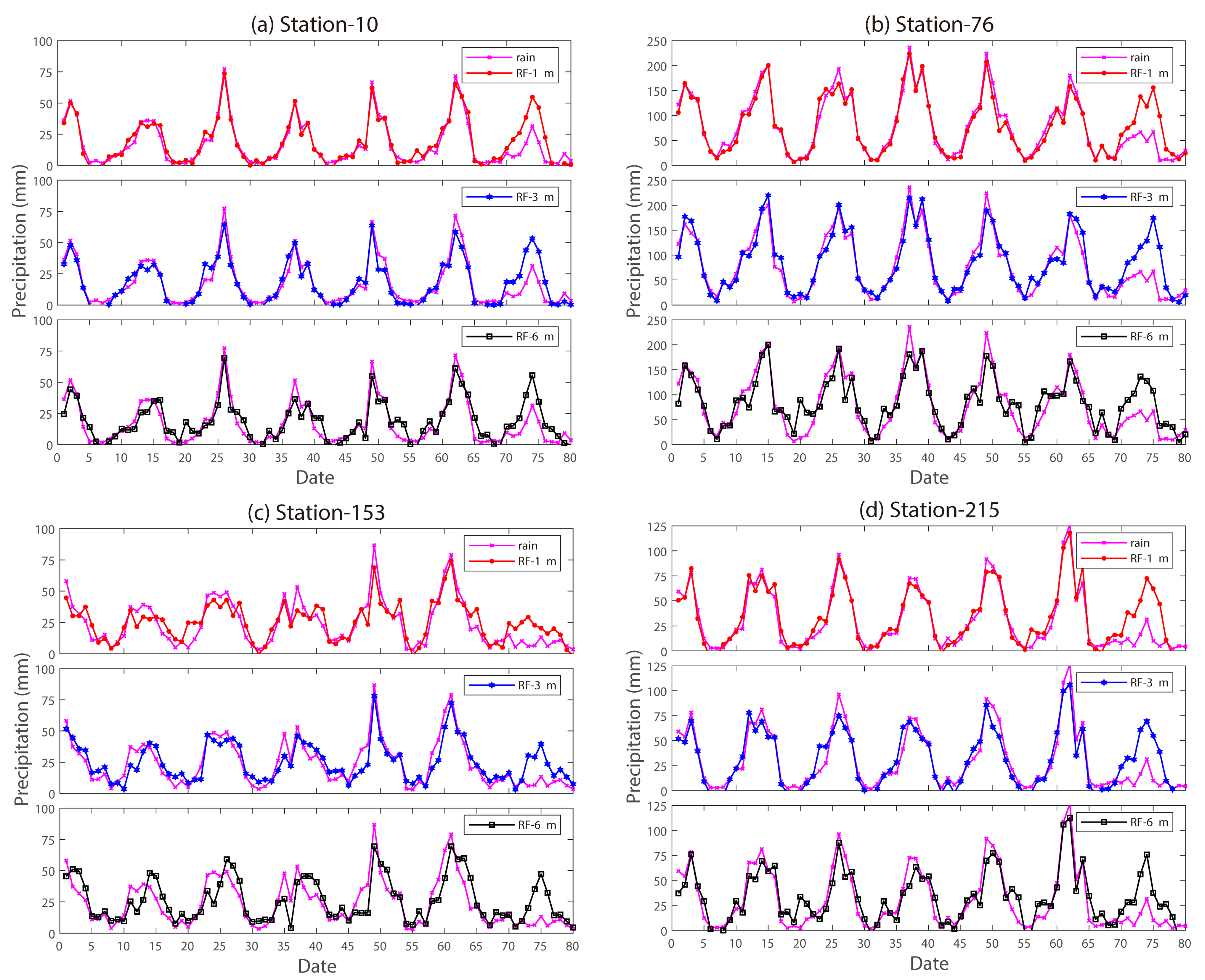
4. Analysis of Precipitation Prediction Results
5. Conclusions
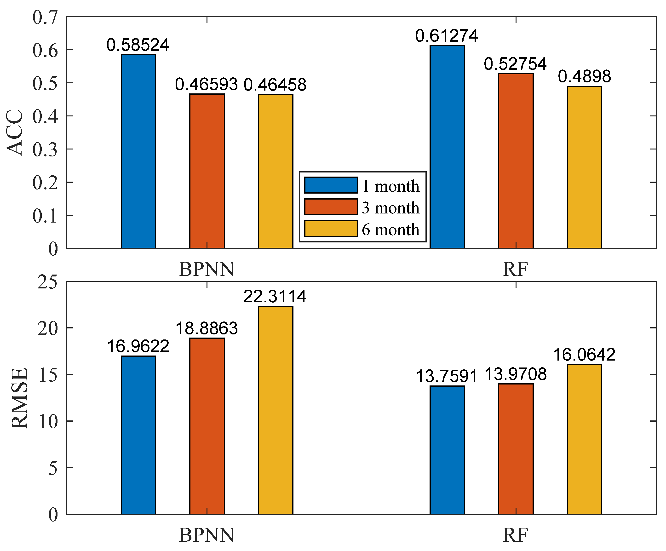
- (1)
- The RF algorithm is significantly better than the BPNN algorithm in terms of prediction, and the predictive ability of both models gradually decreases with the increase in the starting time. The highest average ACC metrics for the model at the three start times are 0.61, 0.53, and 0.49, respectively, corresponding to average RMSE metrics of 13.76, 13.97, and 16.06, respectively. Taking the ACC score (0.53) of the 2022 flood season prediction by the Institute of Atmospheric Sciences of the Chinese Academy of Sciences as a criterion, the precipitation prediction model based on machine learning has high accuracy and is generally able to predict the precipitation trend in western region of China better, and the model has, to a certain extent, improved the prediction ability of 1-month and 3-month precipitation, which can provide a new idea for the short-term climate prediction of precipitation in western China.
- (2)
- Shortcomings: First, although the precipitation prediction model based on machine learning built in this paper can better predict the precipitation in the western region, there is still a gap in the precipitation prediction effect at individual stations. Second, this paper only considers the atmospheric circulation index when screening the best forecasting factors, and does not consider the effect of the sea temperature index and other related indices (e.g., the sunspot index, the number of cold air counts, the Southern Oscillation index, etc.) on precipitation in the western region.
- (3)
- Improvement direction: First, take the sea temperature index into consideration when considering the forecasting factors. Second, try more machine learning algorithms and explore the effect of different machine learning algorithms on precipitation prediction in the western region. Finally, when evaluating the effect of precipitation prediction, more evaluation indexes should be introduced to establish a more sound evaluation system for precipitation prediction.
Author Contributions
Funding
Institutional Review Board Statement
Informed Consent Statement
Data Availability Statement
Conflicts of Interest
Appendix A

| Serial Number | Atmospheric Circulation Index Name |
|---|---|
| 1 | Northern Hemisphere Subtropical High Area Index |
| 2 | North African Subtropical High Area Index |
| 3 | North African-North Atlantic-North American Subtropical High Area Index |
| 4 | Indian Subtropical High Area Index |
| 5 | Western Pacific Subtropical High Area Index |
| 6 | Eastern Pacific Subtropical High Area Index |
| 7 | North American Subtropical High Area Index |
| 8 | Atlantic Subtropical High Area Index |
| 9 | South China Sea Subtropical High Area Index |
| 10 | North American-Atlantic Subtropical High Area Index |
| 11 | Pacific Subtropical High Area Index |
| 12 | Northern Hemisphere Subtropical High Intensity Index |
| 13 | North African Subtropical High Intensity Index |
| 14 | North African-North Atlantic-North American Subtropical High Intensity Index |
| 15 | Indian Subtropical High Intensity Index |
| 16 | Western Pacific Subtropical High Intensity Index |
| 17 | Eastern Pacific Subtropical High Intensity Index |
| 18 | North American Subtropical High Intensity Index |
| 19 | North Atlantic Subtropical High Intensity Index |
| 20 | South China Sea Subtropical High Intensity Index |
| 21 | North American-North Atlantic Subtropical High Intensity Index |
| 22 | Pacific Subtropical High Intensity Index |
| 23 | Northern Hemisphere Subtropical High Ridge Position Index |
| 24 | North African Subtropical High Ridge Position Index |
| 25 | North African-North Atlantic-North American Subtropical High Ridge Position Index |
| 26 | Indian Subtropical High Ridge Position Index |
| 27 | Western Pacific Subtropical High Ridge Position Index |
| 28 | Eastern Pacific Subtropical High Ridge Position Index |
| 29 | North American Subtropical High Ridge Position Index |
| 30 | Atlantic Sub Tropical High Ridge Position Index |
| 31 | South China Sea Subtropical High Ridge Position Index |
| 32 | North American-North Atlantic Subtropical High Ridge Position Index |
| 33 | Pacific Subtropical High Ridge Position Index |
| 34 | Northern Hemisphere Subtropical High Northern Boundary Position Index |
| 35 | North African Subtropical High Northern Boundary Position Index |
| 36 | North African-North Atlantic-North American Subtropical High Northern Boundary Position Index |
| 37 | Indian Subtropical High Northern Boundary Position Index |
| 38 | Western Pacific Subtropical High Northern Boundary Position Index |
| 39 | Eastern Pacific Subtropical High Northern Boundary Position Index |
| 40 | North American Subtropical High Northern Boundary Position Index |
| 41 | Atlantic Subtropical High Northern Boundary Position Index |
| 42 | South China Sea Subtropical High Northern Boundary Position Index |
| 43 | North American-Atlantic Subtropical High Northern Boundary Position Index |
| 44 | Pacific Subtropical High Northern Boundary Position Index |
| 45 | Western Pacific Sub Tropical High Western Ridge Point Index |
| 46 | Asia Polar Vortex Area Index |
| 47 | Pacific Polar Vortex Area Index |
| 48 | North American Polar Vortex Area Index |
| 49 | Atlantic-European Polar Vortex Area Index |
| 50 | Northern Hemisphere Polar Vortex Area Index |
| 51 | Asia Polar Vortex Intensity Index |
| 52 | Pacific Polar Vortex Intensity Index |
| 53 | North American Polar Vortex Intensity Index |
| 54 | Atlantic-European Polar Vortex Intensity Index |
| 55 | Northern Hemisphere Polar Vortex Intensity Index |
| 56 | Northern Hemisphere Polar Vortex Central Longitude Index |
| 57 | Northern Hemisphere Polar Vortex Central Latitude Index |
| 58 | Northern Hemisphere Polar Vortex Central Intensity Index |
| 59 | Eurasian Zonal Circulation Index |
| 60 | Eurasian Meridional Circulation Index |
| 61 | Asian Zonal Circulation Index |
| 62 | Asian Meridional Circulation Index |
| 63 | East Asian Trough Position Index |
| 64 | East Asian Trough Intensity Index |
| 65 | Tibet Plateau Region-1 Index |
| 66 | Tibet Plateau Region-2 Index |
| 67 | India-Burma Trough Intensity Index |
| 68 | Arctic Oscillation |
| 69 | Antarctic Oscillation |
| 70 | North Atlantic Oscillation |
| 71 | Pacific/ North American Pattern |
| 72 | East Atlantic Pattern |
| 73 | West Pacific Pattern |
| 74 | North Pacific Pattern |
| 75 | East Atlantic-West Russia Pattern |
| 76 | Tropical-Northern Hemisphere Pattern |
| 77 | Polar-Eurasia Pattern |
| 78 | Scandinavia Pattern |
| 79 | Pacific Transition Pattern |
| 80 | 30 hPa zonal wind Index |
| 81 | 50 hPa zonal wind Index |
| 82 | Mid-Eastern Pacific 200 mb Zonal Wind Index |
| 83 | West Pacific 850 mb Trade Wind Index |
| 84 | Central Pacific 850 mb Trade Wind Index |
| 85 | East Pacific 850 mb Trade Wind Index |
| 86 | Atlantic-European Circulation W Pattern Index |
| 87 | Atlantic-European Circulation C Pattern Index |
| 88 | Atlantic-European Circulation E Pattern Index |
| Full Name | Acronym |
|---|---|
| Anomalous Correlation Coefficient | ACC |
| Atmospheric Circulation Indices | ACIs |
| Back Propagation Neural Network | BPNN |
| Bayesian Network | BN |
| Convolutional Neural Network | CNN |
| Decision Tree | DT |
| European Centre for Medium-Range Weather Forecasts | ECMWF |
| Empirical Orthogonal Function | EOF |
| Long Short Term Memory | LSTM |
| Machine Learning | ML |
| National Climate Centre | NCC |
| Rotated Empirical Orthogonal Function | REOF |
| Root Mean Square Error | RMSE |
| Support Vector Machine | SVM |
References
- Guo, H.; Li, D.L.; Lin, S.; Dong, Y.X.; Sun, L.D.; Huang, L.N.; Lin, J.J. Temporal and spatial variation of precipitation over western China during 1954–2006. J. Glaciol. Geocryol. 2013, 35, 1165–1175. [Google Scholar]
- Chen, Z.K.; Zhang, S.Y.; Luo, J.L.; Li, Z. Climatic analysis of precipitation anomalies in northwest China. J. Desert Res. 2013, 33, 1874–1883. [Google Scholar]
- Nan, Z.T.; Gao, Z.S.; Li, S.X.; Wu, T.H. Permafrost changes in the northern limit of permafrost on the Qinghai–Tibet Plateau in the last 30 years. Acta Geogr. Sin. 2003, 58, 817–823. [Google Scholar]
- Wu, G.C.; Qin, S.; Hang, C.C.; Ma, Z.S.; Shi, C.M. Seasonal precipitation variability in mainland China based on entropy theroy. Int. J. Climatol. 2021, 41, 5264–5276. [Google Scholar]
- Mai, Z.N.; Xu, D.B.; Xiao, T.G.; Yan, X.J.; Lu, S. Preliminary Study on Probability Forecasting of Flash-Heavy-Rain in Chengdu. Plateau Mt. Meteorol. Res. 2022, 42, 127–134. [Google Scholar]
- Wang, Y.; Li, H.X.; Wang, H.J.; Sun, B.; Chen, H.P. Evaluation of the simulation capability of CMIP6 global climate model for extreme precipitation in China and its comparison with CMIP5. Acta Meteorol. Sin. 2021, 79, 369–386. [Google Scholar]
- Sun, H.; Gao, Z. Prediction of seasonal precipitation based on wavelet analysis and Kriging interpolation. Comput. Electron. Agric. 2020, 177, 105644. [Google Scholar]
- Anaraki, M.V.; Farzin, S.; Mousavi, S.F. Dynamical-statistical hybrid model for seasonal precipitation prediction: A case study of Indus basin, Pakistan. J. Hydrol. 2020, 588, 125010. [Google Scholar]
- Alireza, F.; Saeed, F.; Sayed-Farhad, M. Meteorological drought analysis in response to climate change conditions, based on combined four-dimensional vine copulas and data mining (VC-DM). J. Hydrol. 2021, 603, 127135. [Google Scholar]
- Pan, L.J.; Xue, C.F.; Zhang, H.F.; Gao, X.X.; Liu, M.; Liu, J.H.M. ECMWF precipitation calibration based on the Kalman dynamic frequency matching method. Meteorol. Mon. 2022, 48, 73–83. [Google Scholar]
- Chen, L.L.; Xia, Y. The Influence of Ensemble Size on Precipitation Forecast in a Convective Scale Ensemble Forecast System. J. Appl. Meteorol. Sci. 2023, 34, 142–153. [Google Scholar]
- Wang, Y.T. Precipitation forecast of the Wujiang River Basin based on artificial bee colony algorithm and backpropagation neural network. Alex. Eng. J. 2020, 59, 1473–1483. [Google Scholar] [CrossRef]
- Chen, S.; Sun, Y.N.; Sa, R.N. Research on precipitation prediction based on LSTM and BP neural network. GANSU Water Resour. Hydropower Technol. 2023, 59, 7–11. [Google Scholar]
- Anaraki, M.V.; Farzin, S.; Mousavi, S.-F.; Karami, H. Uncertainty Analysis of Climate Change Impacts on Flood Frequency by Using Hybrid Machine Learning Methods. Water Resour Manag. 2021, 35, 199–223. [Google Scholar] [CrossRef]
- Nakhaei, M.; Mohebbi Tafreshi, A.; Saadi, T. An evaluation of satellite precipitation downscaling models using machine learning algorithms in Hashtgerd Plain, Iran. Model. Earth Syst. Environ. 2023, 9, 2829–2843. [Google Scholar] [CrossRef]
- Huang, C.; Li, Q.P.; Xie, Y.J.; Peng, J.D. Prediction of summer precipitation in Hunan based on machine learning. Trans. Atmos. Sci. 2021, 45, 191–202. [Google Scholar]
- Ashutosh, S.; Manish, K.G. Bayesian network for monthly rainfall forecast: A comparison of K2 and MCMC algorithm. Int. J. Comput. Appl. 2016, 38, 199–206. [Google Scholar]
- Xing, W.; Han, W.Q.; Zhang, L. Improving the prediction of western North Pacific summer precipitation using a Bayesian dynamic linear model. Clim. Dyn. 2020, 55, 831–842. [Google Scholar] [CrossRef]
- Chen, J.P.; Feng, Y.R.; Meng, W.G.; Meng, W.G. A correction method of hourly precipitation forecast based on convolutional neural network. Meteor Mon 2021, 47, 60–70. [Google Scholar]
- Wang, Y.C.; Wei, J.H.; Li, Q.; Qiao, Z.; Yang, K.; Zhu, X.; Bao, S.P.; Wang, Z.J. Radar echo-based study on convolutional recurrent neural network model for precipitation nowcast. Water Resour. Hydropower Eng. 2023, 54, 24–41. [Google Scholar]
- Zhu, K.; Yang, Q.; Zhang, S.; Jiang, S.; Wang, T.; Liu, J.; Ye, Y. Long lead-time radar rainfall nowcasting method incorporating atmospheric conditions using long short-term memory networks. Front. Environ. Sci. 2023, 10, 1054235. [Google Scholar] [CrossRef]
- Li, M.; Liu, K.F. Probabilistic prediction of significant wave height using dynamic bayesian network and information flow. Water 2020, 12, 2075. [Google Scholar] [CrossRef]
- Runge, J.; Bathiany, S.; Bollt, E.; Camps-Valls, G.; Coumou, D.; Deyle, E.; Glymour, C.; Kretschmer, M.; Mahecha, M.D.; Muñoz-Marí, J.; et al. Inferring causation from time series in Earth system sciences. Nat. Commun. 2019, 10, 2553. [Google Scholar] [CrossRef]
- Marlene, K.; Dim, C.; Donges, J.F.; Runge, J. Using Causal Effect Networks to Analyze Different Arctic Drivers of Midlatitude Winter Circulation. J. Clim. 2016, 29, 4069–4081. [Google Scholar]
- McGraw, M.C.; Barnes, E.A. New Insights on Subseasonal Arctic–Midlatitude causal connections from a regularized regression model. J. Clim. 2020, 33, 213–228. [Google Scholar] [CrossRef]
- Li, M.; Zhang, R.; Liu, K.F. Machine learning incorporated with causal analysis for short-term prediction of sea ice. Front. Mar. Sci. 2021, 8, 649378. [Google Scholar] [CrossRef]
- Zhang, Y.; Liang, X.S. The causal role of South China Sea on the Pacific–North American teleconnection pattern. Clim. Dyn. 2022, 59, 1815–1832. [Google Scholar] [CrossRef]
- Docquier, D.; Vannitsem, S.; Ragone, F.; Wyser, K.; Liang, X.S. Causal links between Arctic Sea ice and its potential drivers based on the rate of information transfer. Geophys. Res. Lett. 2022, 49, e2021GL095892. [Google Scholar] [CrossRef]
- Luo, W.; Yin, H.; Yang, S.; Zhou, Y.; Ran, L.; Jiao, B.; Lai, Z. Response of a westerly-trough rainfall episode to multi-scale topographic control in southwestern China. Atmos. Ocean. Sci. Lett. 2022, 15, 100148. [Google Scholar] [CrossRef]
- Zhu, J.T.; Yang, Q.Y.; Li, X.; Li, Y. Characteristics and East Downscaling Forecast Model of Summer Precipitation in Northwest China. Plateau Meteorol. 2023, 42, 646–656. [Google Scholar]
- Liang, X.S. Unraveling the cause-effect realation between time series. Phys. Rev. E 2014, 90, 052150. [Google Scholar] [CrossRef] [PubMed]
- Liang, X.S. Normalizing the causality between time series. Phys. Rev. E 2015, 92, 022126. [Google Scholar] [CrossRef] [PubMed]
- Peng, J.B.; Zheng, F.; Fan, F.X.; Chen, H.; Lang, X.M.; Zhan, Y.L.; Lin, C.H.; Zhang, Q.Y.; Lin, R.P.; Li, C.F.; et al. Climate Prediction and Outlook in China for the Flood Season 2022. Clim. Environ. Res. 2022, 27, 547–558. [Google Scholar]
| Model | 1 | 2 | 3 | 4 | 5 | 6 | 7 | 8 |
| Expvar | 56.7 | 10.6 | 4.1 | 2.6 | 1.1 | 0.9 | 0.6 | 0.5 |
| Index | Index | ||||
|---|---|---|---|---|---|
| 1 | 0.499 | 0.316 | 45 | 0.069 | 0.000 |
| 2 | 0.539 | 0.378 | 46 | 0.049 | 0.348 |
| 3 | 0.534 | 0.382 | 47 | 0.144 | 0.155 |
| 4 | 0.013 | 0.010 | 48 | 0.141 | 0.326 |
| 5 | 0.063 | 0.002 | 49 | 0.061 | 0.189 |
| 6 | 0.094 | 0.242 | 50 | 0.009 | 0.360 |
| 7 | 0.279 | 0.339 | 51 | 0.551 | 0.419 |
| 8 | 0.411 | 0.378 | 52 | 0.366 | 0.389 |
| 9 | 0.005 | 0.017 | 53 | 0.220 | 0.360 |
| 10 | 0.448 | 0.368 | 54 | 0.003 | 0.317 |
| 11 | 0.013 | 0.142 | 55 | 0.552 | 0.412 |
| 12 | 0.318 | 0.303 | 56 | 0.001 | 0.011 |
| 13 | 0.547 | 0.361 | 57 | 0.088 | 0.020 |
| 14 | 0.418 | 0.352 | 58 | 0.537 | 0.405 |
| 15 | 0.015 | 0.014 | 59 | 0.045 | 0.234 |
| 16 | 0.068 | 0.024 | 60 | 0.044 | 0.019 |
| 17 | 0.047 | 0.205 | 61 | 0.034 | 0.186 |
| 18 | 0.112 | 0.312 | 62 | 0.041 | 0.030 |
| 19 | 0.135 | 0.331 | 63 | 0.001 | 0.003 |
| 20 | 0.001 | 0.012 | 64 | 0.515 | 0.428 |
| 21 | 0.158 | 0.329 | 65 | 0.313 | 0.100 |
| 22 | 0.016 | 0.104 | 66 | 0.099 | 0.323 |
| 23 | 0.370 | 0.523 | 67 | 0.045 | 0.134 |
| 24 | 0.057 | 0.332 | 68 | 0.005 | 0.007 |
| 25 | 0.317 | 0.137 | 69 | 0.004 | 0.008 |
| 26 | 0.254 | 0.253 | 70 | 0.002 | 0.005 |
| 27 | 0.403 | 0.520 | 71 | 0.008 | 0.014 |
| 28 | 0.309 | 0.002 | 72 | 0.020 | 0.006 |
| 29 | 0.315 | 0.204 | 73 | 0.010 | 0.013 |
| 30 | 0.186 | 0.048 | 74 | 0.020 | 0.027 |
| 31 | 0.352 | 0.527 | 75 | 0.012 | 0.014 |
| 32 | 0.296 | 0.255 | 76 | 0.000 | 0.000 |
| 33 | 0.396 | 0.518 | 77 | 0.007 | 0.012 |
| 34 | 0.286 | 0.063 | 78 | 0.001 | 0.025 |
| 35 | 0.132 | 0.190 | 79 | 0.001 | 0.002 |
| 36 | 0.187 | 0.202 | 80 | 0.055 | 0.039 |
| 37 | 0.067 | 0.017 | 81 | 0.000 | 0.000 |
| 38 | 0.336 | 0.528 | 82 | 0.257 | 0.206 |
| 39 | 0.075 | 0.000 | 83 | 0.039 | 0.086 |
| 40 | 0.189 | 0.154 | 84 | 0.053 | 0.058 |
| 41 | 0.130 | 0.014 | 85 | 0.029 | 0.006 |
| 42 | 0.176 | 0.306 | 86 | 0.141 | 0.115 |
| 43 | 0.200 | 0.096 | 87 | 0.132 | 0.128 |
| 44 | 0.338 | 0.459 | 88 | 0.002 | 0.000 |
| ML Algorithms | Parameterization |
|---|---|
| BPNN | Number of input layer nodes: 72, 69, 41 and 42 Number of implicit layer nodes: First mode: {9, 10, 11, …, 18} Second mode: {9, 10, 11, …, 18} Third mode: {7, 8, 9, …, 16} Fourth mode: {7, 8, 9, …, 16} Number of output layer nodes: 1 |
| RF | Number of decision trees: 500 Minimum leaves number: 5 |
| ACC | BPNN | RF | ||||
|---|---|---|---|---|---|---|
| 1 Month | 3 Month | 6 Month | 1 Month | 3 Month | 6 Month | |
| 0 | 22 | 18 | 0 | 0 | 0 | |
| 47 | 37 | 57 | 42 | 56 | 56 | |
| 25 | 29 | 20 | 22 | 25 | 31 | |
| 22 | 35 | 18 | 25 | 33 | 42 | |
| 72 | 97 | 126 | 63 | 69 | 86 | |
| 74 | 20 | 1 | 88 | 57 | 25 | |
| RMSE | BPNN | RF | ||||
|---|---|---|---|---|---|---|
| 1 Month | 3 Month | 6 Month | 1 Month | 3 Month | 6 Month | |
| 10 | 9 | 17 | 11 | 23 | 10 | |
| 80 | 75 | 64 | 93 | 71 | 92 | |
| 56 | 48 | 24 | 68 | 54 | 56 | |
| 50 | 54 | 33 | 56 | 89 | 42 | |
| 34 | 36 | 65 | 10 | 3 | 30 | |
| 10 | 18 | 37 | 2 | 0 | 10 | |
Disclaimer/Publisher’s Note: The statements, opinions and data contained in all publications are solely those of the individual author(s) and contributor(s) and not of MDPI and/or the editor(s). MDPI and/or the editor(s) disclaim responsibility for any injury to people or property resulting from any ideas, methods, instructions or products referred to in the content. |
© 2023 by the authors. Licensee MDPI, Basel, Switzerland. This article is an open access article distributed under the terms and conditions of the Creative Commons Attribution (CC BY) license (https://creativecommons.org/licenses/by/4.0/).
Share and Cite
Li, H.; Li, M. Modeling of Precipitation Prediction Based on Causal Analysis and Machine Learning. Atmosphere 2023, 14, 1396. https://doi.org/10.3390/atmos14091396
Li H, Li M. Modeling of Precipitation Prediction Based on Causal Analysis and Machine Learning. Atmosphere. 2023; 14(9):1396. https://doi.org/10.3390/atmos14091396
Chicago/Turabian StyleLi, Hongchen, and Ming Li. 2023. "Modeling of Precipitation Prediction Based on Causal Analysis and Machine Learning" Atmosphere 14, no. 9: 1396. https://doi.org/10.3390/atmos14091396
APA StyleLi, H., & Li, M. (2023). Modeling of Precipitation Prediction Based on Causal Analysis and Machine Learning. Atmosphere, 14(9), 1396. https://doi.org/10.3390/atmos14091396