Abstract
Buildings are responsible for a large part of energy demand worldwide. To collaborate to reduce this demand, this paper aims to present a computational model to analyze the performance of an earth–air heat exchanger (EAHE) based on computational fluid dynamics using the ANSYS/Fluent® software in the simulations. This passive air conditioning system uses the soil as a heat exchanger, taking advantage of the fact that the temperature of the soil at a certain depth remains relatively constant, regardless of the weather conditions above the surface, promoting heating, cooling, or ventilation for buildings. The air temperature values obtained were compared with experimental data from sensors installed in an EAHE at the Federal University of Technology—Parana, Ponta Grossa/Brazil (25.1° South, 50.16° West) to validate the computational model. A high computational effort would be demanded to perform these simulations involving the whole soil domain and the climatic boundary conditions. In order to optimize the numerical analysis of EAHE, two reduced models for the soil and heat exchanger domains were verified. First, a constant temperature of 23.7 °C was imposed on the surface of the exchanger tube, corresponding to the average soil temperature at a depth of 1.5 m. Afterward, a reduced soil domain extending 0.5 m in all directions from the heat exchanger serpentine was considered. Likewise, constant temperatures were imposed on the upper and lower surfaces of the soil domain, also obtained experimentally. In both cases, the temperature values obtained through the fast simulations showed good agreement compared to the experimental values. Barely explored in the literature, the thermal behavior of the two identical indoor environments at the university was also compared, in which the climatized environment, with the EAHE working in a closed loop, obtained milder and smaller amplitude air temperatures.
1. Introduction
Currently, there is a great demand for more sustainable alternatives to meet human needs involving the expenditure of electricity since energy consumption is growing every year worldwide. In Brazil, commercial, residential, and public buildings were responsible for 51.2% of the total annual electricity consumption, according to the 2021 National Energy Balance [1].
Besides being a sustainable alternative in civil construction with an emphasis on the air conditioning field, the earth–air heat exchanger (EAHE) can also reduce electricity costs and ensure thermal comfort in environments. This device takes advantage of the high thermal inertia of the soil, where it can maintain a practically constant temperature at specific depths, thus allowing it to heat the air on cold days and cool it on hot days. This type of process can be called passive climatization; its operation consists of moving the air through underground pipes before leading it to the environment, causing it to exchange heat with the soil, thus, having the only expenditure of energy with the circulation of the air through a fan.
Many authors describe the EAHE as an efficient way to reduce air conditioning costs. For example, Vaz [2] carried out an experimental and numerical study of an EAHE, conducted in southern Brazil in the city of Viamão. The results showed that the heat exchanger used for heating reached up to 3 °C temperature increase, with the prospect of reaching 8 °C. For cooling, the potential would get to 4 °C for the analyzed climate. Maoz et al. [3] used the response surface method (RSM) to optimize a open loop earth–air heat exchanger (EAHE) system installed in Peshawar city in Pakistan. Parametric analysis was conducted for the three variables: pipe length, diameter, and air velocity. A regression equation also was developed to predict the cooling load considering the weather and soil conditions.
Greco and Masselli [4] researched the parameters that optimize the thermal performances of a horizontal single-duct EAHE installed in Naples, Italy. Geometrical characteristics, such as the pipe length, diameter, burial depth, and the thermal and flow parameters of humid air were studied. The work showed that the thermal performance of the EAHE increased with length until the saturation distance was reached, with smaller diameters and slower air flows. Peña and Ibarra [5] evaluated the energy saving obtained by installing an EAHE in a tropical climate in Colombia. A mathematical model was implemented in TRNSYS® software to predict the heat exchanger’s thermal performance and cooling capacity. Parameters such as the pipe length, diameter, material, thickness, airflow mass, soil, local atmospheric conditions, building features, and economic feasibility of the project were verified.
In Abadie et al. [6], the heating and cooling potentials of a heat exchanger in three cities in southern Brazil (Porto Alegre, Curitiba, and Florianópolis) were numerically analyzed using the building energy simulation tool (TRNSYS®). The study showed that climatic conditions and solar radiation must be considered in the calculations. Furthermore, Curitiba, located 100 km from where our study was conducted with very similar soil and climatic conditions, obtained the best results.
Serageldin et al. [7] developed a parametric study of an EAHE through simulations in ANSYS/Fluent® to analyze the effects of the dimensions and material of the pipes on the thermal performance. The authors concluded that the increased tube diameter promotes decreased air temperature at the EAHE exit due to a rise in the contact surface between the tube and air. In addition, the authors found that increasing air velocity decreases the heat transfer rate with the soil. Regarding the pipe material, minimal differences between the results were observed, in which PVC (polyvinyl chloride) was indicated as a good option due to its lower cost. Elminshawy et al. [8] conducted an experimental study of a heat exchanger using a copper tube where air circulated at a controlled temperature. The authors evaluated the thermal performance of three soils regarding their compaction and verified the application in arid and hot places. The most compact soil presented the best performance, and the intermediate one, the worst, for cooling effects.
Liu et al. [9] studied the thermal performance of EAHE in hot summer and cold winter areas in Changsha, China. The influence of the soil, supply air, and outdoor air temperatures in the COP and heat transfer were analyzed for one week.
Menhoudj et al. [10] used an experimental model of an EAHE installed in Algeria and validated the numerical model using TRNSYS® to evaluate the thermal performance by optimizing some constructive parameters: length, depth of installation, and diameter of the pipe. A length of 25 m, a depth of 2 m, and a diameter of 120 mm were the optimal values obtained. In this study, the test cell corresponded to two adjoining rooms having the same geometric dimensions: 4.7 m × 3.7 m × 2.8 m. In the first room, the energetic performance of a direct solar floor was tested, whereas the second was used as a reference room in which measure instrumentations were installed.
Li [11] analyzed the effectiveness of an EAHE experimentally located in Songbei District, Harbin, China, where the air temperature showed an average decrease of 14.6 °C, and the average total cooling capacity was 8792. W. Liu et al. [12] proposed an experimental study in a vertical earth-to-air heat exchanger system (VEAHE) to validate its thermal and economic feasibility. The energy metrics analysis indicated that the proposed system was economically viable.
Congedo [13] presented the experimental validation of a mathematical model implemented using CFD Fluent for the simulation of an EAHE located in Rubiana, Turin, Italy. The authors observed that the transient thermal performance of the EAHE was independent of the thermal conductivity of the soil but was dependent on burial depth.
Tang et al. [14] developed a time-saving numerical model on the MATLAB/Simulink® platform. The experimental validation results indicated that the maximum absolute relative deviation was 3.18% between the model results and the experimental data. Several parametrical influences in the heat transfer performance also were carried out. Hegazi et al. [15] developed analytical solutions for EAHE systems to predict and optimize the effects of different parameters on the outlet air temperature that supplies the air-cooling unit in an operation room in a hospital in Egypt. The performance of the cooling system was evaluated in terms of compressor power consumption, overall power savings, overall cost reduction, and payback period. The maximum reduction in compressor power consumption and annual costs was estimated to be 44% and 16.6%, respectively.
Hacini et al. [16] validated a numerical study from experimental data found in the literature. The authors also compared the performance of an EAHE in three regions of Algeria: Jijel (humid climate), Djelfa (semi-arid climate), and Timimoun (desert climate), each with a different soil type. The study concluded that a depth of 5 m should be used in Timimoun, and 2 m for other locations, with pipe lengths of 45 m, 30 m, and 30 m, respectively. Furthermore, the cooling potential for a typical hot day was estimated to be 26.21 kWh, 13.83 kWh, and 7.66 kWh for Timimoun, Djelfa, and Jijel, respectively.
Vivas and Guerra [17] developed a three-dimensional numerical model of the EAHE using ANSYS/Fluent® to evaluate the influence of airflow velocity, length, and diameter of the pipe on the thermal performance of this system adapted to climatic conditions and the soil characteristics of Belém City, in Brazil. From the results obtained, a maximum relative difference of 4.14% was verified between the experimental and computational data. Furthermore, they concluded that using lower airflow velocities reduces the length needed to obtain a specific decrease in temperature.
Nejad et al. [18] numerically investigated the use of an underground air-conditioning tunnel for Tehran’s climate also using the ANSYS/Fluent® software. The results showed that the heat exchanger created comfortable conditions except for a short period of the day. The work also verified that due to the thermal saturation of the soil, the system was not suitable for continuous work, and a depth of 3 m was appropriate to bury the pipe to prevent the effect of ground surface heat. Qi et al. [19] evaluated the effect of humidity and condensation on the thermal performance of an EAHE using CFD. The distribution of relative humidity in the pipe, the impact of inlet air relative humidity, the effects of inlet air temperature, and the volume flow rate on the performance of the heat exchanger were analyzed. The authors observed that condensation had little effect on the airflow distribution uniformity of the EAHE, and the humid air in a small-diameter pipe tended to condense more easily. The influence of the configurations on the air condensation’s performance was also verified.
Zeitoun et al. [20] studied an EAHE system built at the University of Strasbourg in the northeast of France using energy and exergy analyses for a typical heating period. Results showed that the heat energy gained using the system was around 63 kWh and that the exergetic efficiency of the system was about 57% on average. The authors also verified that the exergy was mainly destroyed in the fan, while the lowest destruction was in the filter.
Considering the applicability of EAHE in ventilation systems, Liu et al. [21] reviewed the state-of-the-art of shallow geothermal ventilation (SGV) systems for building thermal performance enhancement. The authors showed that with a small initial investment cost, this system is a promising technology to partly replace the conventional air-conditioning system for air pre-cooling or pre-heating. Amanowicz et al. [22] also described the recent advancements in ventilation systems to decrease energy consumption in buildings. In this review of the literature, we considered articles that were published in the last three years.
Based on these studies, the present work aimed to develop a computational model using ANSYS/Fluent® software to obtain air temperature gradients in an EAHE submitted for different boundary conditions, using a reduced soil domain, in order to decrease the time computationally. Validation of the computational model used in the simulations was also performed through comparison with experimental results obtained at the EAHE installed at UTFPR (Federal University of Technology—Parana) in Ponta Grossa, Brazil. Finally, the thermal behavior of the two identical indoor environments (with and without the EAHE installed) was compared. The EAHE presented a good cooling performance in the climatized environment for the analyzed summer period.
2. Methodology
Simulations in this work were performed using the version 2021 ANSYS/Fluent® commercial software. The governing equations, boundary conditions, geometry and mesh, and EAHE constructive details will be presented in this section.
2.1. Considerations and Equations
Although the variation of air properties with temperature could affect the performance of the EAHE [23], in this study, the air was considered incompressible and with constant properties. Therefore, the continuity equation, obtained from Tannehill et al. [24], is expressed in Equation (1),
in which is the velocity vector of the fluid (m/s).
Following the same previous considerations and considering no external force acting, the equation of conservation of momentum (Navier–Stokes) is described by Equation (2),
in which is the specific mass of the fluid (kg/m3), is the static pressure (N/m2), is the gravity acceleration (m/s2), and is the dynamic viscosity (kg/m.s).
The energy equation, according to the hypotheses already adopted, is defined by Equation (3),
in which is the internal energy per unit mass (J/kg), is the heat transferred from external agents per unit volume (J/m3), is the coefficient of thermal conductivity (W/mK), is the temperature (K), and is the energy dissipation rate (W/m3).
For turbulence, the standard k-ε model was used, which was used in the works by Misra et al. [25], and consists of two equations, described by Equations (4) and (5),
and,
where corresponds to the turbulent kinetic energy (J/kg), is the turbulent viscosity (kg/m.s), is the turbulent energy dissipation rate (m2/s3), is the turbulent Prandtl number for , is the turbulent Prandtl number for , is the turbulent kinetic energy generation due to mean velocity gradients () and is the turbulent kinetic energy generation due to buoyancy ().
The turbulent viscosity term () is calculated as a function of k and ε, as expressed in Equation (6):
The constants used in the turbulence model were predefined by the software with the following values: , , , , and .
2.2. Geometry, Mesh, and Boundary Conditions
The dimensions and the geometry of the EAHE, shown in Table 1 and Figure 1, are based on previous work performed by Vasconcellos and Santos [26]:

Table 1.
EAHE dimensions.
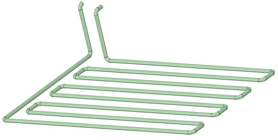
Figure 1.
Geometry of the air path.
A reduced model for the soil domain was used in the simulations to analyze the mesh sensitivity with an optimized computational time. Considering the serpentine shape of the heat exchanger used in this work, a soil domain of dimensions 6.7 m × 4.75 m × 1 m was considered, as shown in Figure 2.
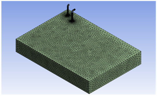
Figure 2.
Geometry and mesh of the soil domain.
The domain of the piping material was not considered in simulations to avoid distortions in mesh generation, as adopted in the work of Shojaee and Malek [27]. Due to the low thermal resistance presented by the pipe wall, the presence of this domain did not cause significant changes in the results.
An automatically generated mesh with 3,683,460 elements (ground plus air domain) was used in the simulations as a default. Some mesh sizes were tested to verify the independence of the numerically obtained results. Four tests were performed, with changes in the number of air domain elements and the soil plus air domains. Table 2 shows the number of elements used in the tests and the maximum temperature difference for 23 January 2022, concerning the experimental values, considering all sensors distributed along the heat exchanger.
Table 2.
Meshes used in the sensitivity analysis.
According to Table 2, there is no significant difference between the meshes in the accuracy of the results. The difference in computational time using the four meshes was also insignificant, so the mesh default was used in all simulations.
As mentioned, the experimental data analyzed in this work were obtained on 23 January 2022. Unlike other years, the summer of 2021–2022 was mild in Ponta Grossa, Brazil (25.1° South, 50.16° West), and this day corresponded to the highest temperature ranges in the climate for the heat exchanger installation site. The temperature and solar irradiance values on this date are shown in Figure 3.
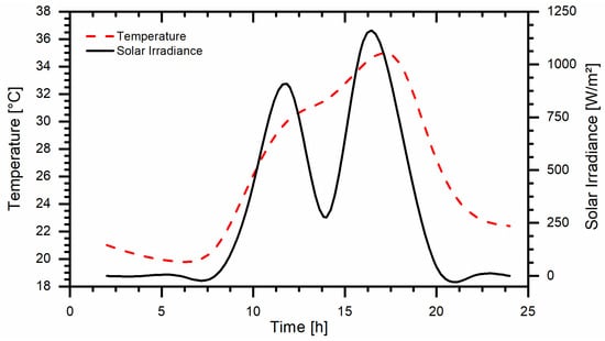
Figure 3.
Temperature and solar irradiance values on 23 January 2022.
The thermophysical properties of air and soil were considered constant. The soil in the EAHE installation region is of the clay type, with properties similar to those given by Oke [28] (dry basis). Table 3 shows the physical properties of the air and the soil used for the simulations.
Table 3.
Air and soil physical properties.
The air inlet temperatures in the EAHE were interpolated using the least squares method, and with these polynomials, a UDF (user-defined function) was developed to apply them in the simulations as an inlet condition. Concerning inlet velocity and outlet condition (gauge pressure), values of 0.774 m/s and 0 Pa were used, respectively.
Two hypotheses were verified for optimizing the simulation time. First, the soil domain was disregarded, assigning a constant temperature on the pipe surface. In the second hypothesis, a ground domain was set, extending 0.5 m from the pipe surface in all directions, as shown in Figure 2.
For the simulation without a soil domain, a constant temperature of 23.7 °C was considered for the wall of the pipes, whose average value was obtained experimentally for 1.5 m of depth.
The side walls were considered adiabatic for the simulations with the soil domain; the upper and lower surfaces were adopted with 24 °C and 23.5 °C, obtained at 1 and 2 m of depth, respectively.
2.3. Experimental Apparatus
Figure 4 shows the experimental apparatus constructed with PVC tubes of 100 mm diameter in serpentine configuration, with tubes 5.15 m long placed at every 0.5 m. The piping was assembled at 1.5 m below ground level, with a total length of 50.65 m, where the temperatures were obtained using 14 Omega Engineering® type K thermocouples installed along EAHE (indicated in Figure 4). The data acquisition bench comprised a Keysight® DAQ970A, two Keysight® DAQM901A 20 channel multiplexers, and a microcomputer with an Intel® Core i7-7600 processor.
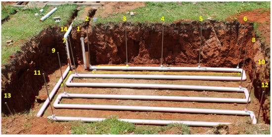
Figure 4.
Thermocouples installed in the EAHE.
The forced airflow was inflated by a system composed of an AeroMack® radial fan CRE-03 with a power of 1.5 kW and a maximum flow of 3.2 m3/min, installed between the space of the heat exchanger and laboratory where the data acquisition bench was positioned. Climatic data such as temperature, wind speed, and relative humidity were obtained through an Instrutemp® ITWH-1080 meteorological station. A Kipp and Zonen® CMP3 pyranometer has been used for solar irradiance. Table 4 presents the experimental uncertainties regarding the measured quantities.
Table 4.
Measurement uncertainties.
2.4. Indoor Environments
The cooling capacity of the EAHE in an indoor environment (2.12 m × 2.76 m × 3.30 m) of the Graduate Program in Mechanical Engineering building was evaluated, comparing the thermal behavior to another identical environment without air conditioning, as identified in Figure 5 and Figure 6. These two rooms are made of masonry, without windows, with access through aluminum doors, which remain closed during data acquisition. Two K-type thermocouples were positioned in each environment to obtain the air temperature.
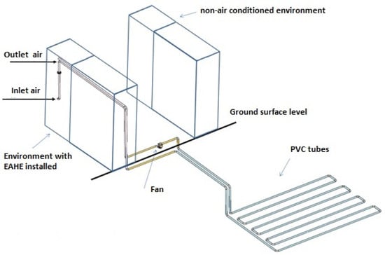
Figure 5.
Indoor environments of the Graduate Program in Mechanical Engineering building.
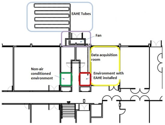
Figure 6.
Location of indoor environments within the building.
Figure 6 indicates the location within the building. In the region indicated in yellow, the control and data acquisition equipment was installed. In the region in red, the air inlet and outlet tubes in the air-conditioned environment are placed, and in green, the environment is without air conditioning. In the outer region of the building, indicated in purple, there is a fan for air circulation, and the heat exchanger tubes are indicated in blue.
3. Results
First, the results were validated by comparing experimental and computational values on 23 January 2022. The chosen section is located 5.95 m away from the heat exchanger inlet, where the most significant temperature gradients were found. The maximum absolute relative deviation (MARD), as shown in Equation (7), has been used for the analyses [14].
where j is the number of selected data samples, and Tj,sim and Tj,exp are the simulated and experimental air temperatures, respectively.
As seen in Figure 7, 3.1% was the most considerable relative difference between experimental and computational values obtained at 5 p.m. According to the comparison between the results, the numerical model presented showed good agreement with the monitored values.
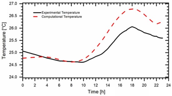
Figure 7.
Comparison between experiment and simulation data in the section located 5.95 m away from the heat exchanger inlet.
After the validation of the computational model, simulations were performed considering the hypothesis without the soil domain and the surface of the air domain with a constant temperature of 23.7 °C. Figure 8 shows the average temperature profile along the heat exchanger. The maximum relative difference between experimental and computational results near the heat exchanger outlet was of 2.6% (0.6 °C). A computational time of 15 min was required using to the simulations a computer with an Intel® Core i5-9400f processor, 16 GB of RAM, and a Nvidia® GeForce GTX 1060 video card with 3 GB of memory.
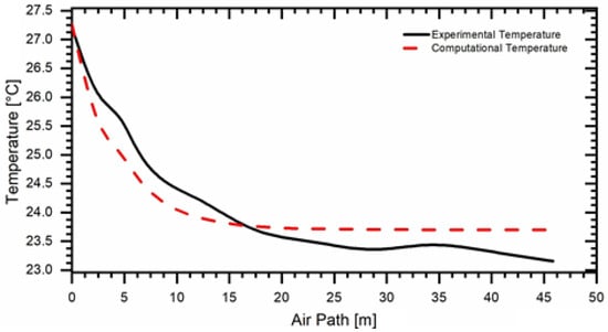
Figure 8.
Comparison between the computational and experimental average air temperatures in the EAHE.
In order to improve the results without compromising computational time, a reduced soil domain was also used in the simulations. For this hypothesis, at the same time and day, the results obtained are shown in Figure 9. The simulation time was 30 min. The better similarity of behavior between the two curves also had the highest maximum relative difference of 2.6%.
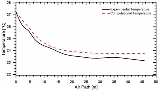
Figure 9.
Comparison of the computational and experimental average air temperatures in the EAHE considering the soil domain.
The decrease in experimental temperature of 0.5 °C observed in Figure 8 and Figure 9 at the end of the heat exchanger was attributed to the position of the last sensor, close to the soil surface. As also seen in Figure 10, the air practically reached thermal equilibrium after 25 m of tube length.
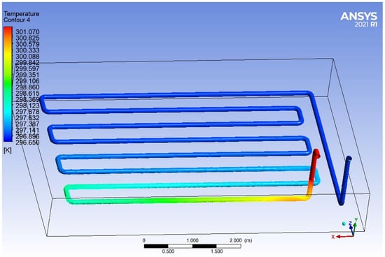
Figure 10.
Air temperature along the EAHE, at 2 p.m., on 23 January 2022.
The temperature profile around the cross-section of the tubes noticed in Figure 11 shows that the spacing of 0.5 m between the passes was sufficient to ensure the good performance of the heat exchanger.
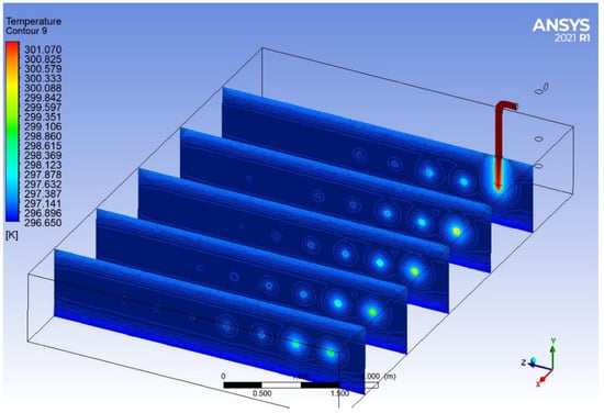
Figure 11.
Air and soil temperature at 2 p.m., on 23 January 2022.
With the computational results having a good approximation with the experimental values, the model considering the hypothesis with soil domain was used to analyze the performance of the EAHE in conditions different from those recorded experimentally. Simulations were carried out using the same boundary conditions for the soil domain but increasing and reducing the inlet temperature by 10 °C to verify the performance of the EAHE in more extreme temperature conditions. Figure 12 shows the performance of the EAHE, on 23 January 2022, for these hypotheses.
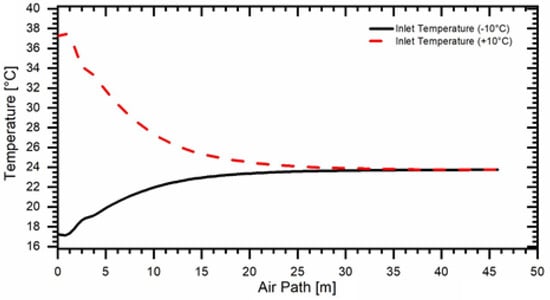
Figure 12.
EAHE performance with a rise and decrease of 10 °C in the inlet temperature.
Average temperatures of 6.5 °C and 13.3 °C were obtained for the heating and cooling, respectively. Furthermore, Figure 12 shows that the air reaches thermal equilibrium at 23.7 °C. It is also observed that a 25 m long pipe would be sufficient to guarantee thermal equilibrium between the soil and the air in the heat exchanger. However, for long continuous periods of device use, a greater length is necessary to avoid the thermal saturation of the soil.
The air temperature of two environments are compared in Figure 13. In the conditioned environment, the temperature remained practically stable at around 25.5 °C. The unconditioned environment presented a peak temperature of approximately 28 °C at 6 p.m.
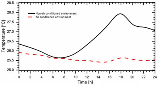
Figure 13.
Air temperature of the indoor environments on 23 January 2022.
As the summer was mild during the period analyzed in this work, after 23 January 2022, two 1.5 kW oil heaters were inserted in both environments to test the performance of the EAHE. Figure 14 shows temperatures above 35 °C for the non-air-conditioned environment. In the case of the air-conditioned environment, the maximum air temperature was 28.3 °C. Even with a high internal heat generation for the dimensions of the environments analyzed, the heat exchanger presented a good performance. Therefore, the EAHE could be used for more severe climatic conditions, as also observed in Figure 12.
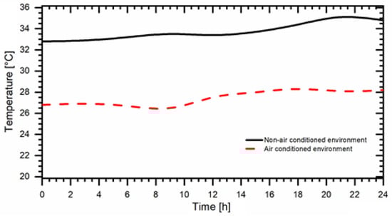
Figure 14.
Air temperature of the indoor environments with oil heaters.
4. Conclusions
With the growing demand for more sustainable alternatives, the earth–air heat exchanger (EAHE) emerges as an alternative to conventional climatization methods. In this sense, the present work was dedicated to obtaining a computational model and submitted to a physical validation to verify the thermal performance of this system. With the comparison made between the computational and experimental results, a good similarity was verified, obtaining, for the analyzed conditions, a maximum difference of 3.1%. Therefore, the reduced model used for the soil domain proved to be adequate for the EAHE simulations to decrease the computational time, avoiding the use of the local climatic conditions as a boundary condition. Thus, average soil temperatures estimated or obtained experimentally could be used.
Based on the conditions of the validated computational model, a simulation was carried out by adding 10 °C to the inlet condition, obtaining an average reduction of 13.3 °C. Likewise, a simulation was carried out with a 10 °C decrease in temperature as an input condition, causing the EAHE to perform air heating, reaching an increase of 6.5 °C. In both cases, the thermal behavior of the air was verified, which, when it reaches thermal equilibrium with the ground, tended to a temperature of 23.7 °C from 25 m of pipe length. When the indoor air temperatures of the two environments were compared, the air-conditioned environment presented better thermal comfort conditions, even with high internal heat generation. Through the results obtained, this work showed that the EAHE presented an excellent thermal performance, taking advantage of the high thermal inertia of the soil to keep the air temperature practically constant and close to the comfort temperature.
Author Contributions
For this research, the individual contributions are as follows: Conceptualization, C.H.D. and G.H.d.S.; methodology, G.H.d.S. and T.A.A.; software, G.C.C.; validation, C.H.D. and V.V.D.; investigation, C.H.D. and V.V.D.; resources, C.H.D.; writing—original draft preparation, C.H.D.; writing—review and editing, G.H.d.S. and T.A.A.; visualization, T.A.A. and V.V.D.; supervision, G.H.d.S.; funding acquisition, T.A.A. All authors have read and agreed to the published version of the manuscript.
Funding
This research was supported by the Federal University of Technology—Parana and Brazilian agencies: Coordination for the Improvement of Higher Education Personnel (CAPES)—Financing Code 001, and Brazilian National Council for Scientific and Technological Development (CNPq), process numbers 409631/2021-3 and 312367/2022-8.
Institutional Review Board Statement
Not applicable.
Informed Consent Statement
Not applicable.
Data Availability Statement
Not applicable.
Conflicts of Interest
The authors declare no conflict of interest.
Nomenclature
| heat transferred [J/m3] | |
| thermal conductivity [W/(m.K)] | |
| constant 1 (turbulence model) [-] | |
| constant 2 (turbulence model) [-] | |
| constant 3 (turbulence model) [-] | |
| turbulent viscosity constant [-] | |
| turbulent Kinetic Energy [J/kg] | |
| internal energy [J/kg] | |
| specific mass [kg/m3] | |
| turbulent Prandtl number for [-] | |
| turbulent Prandtl number for 𝜖 [-] | |
| fluid static pressure [N/m2] | |
| turbulent energy dissipation [m2/s3] | |
| transfer rate of mechanical energy in the fluid deformation process due to viscosity [W/m3] | |
| coefficient of thermal conductivity [W/(m.K)] | |
| temperature [K] | |
| time [s] | |
| vector speed [m/s] | |
| dynamic viscosity [kg/(m.s)] | |
| turbulent viscosity [kg/(m.s)] | |
| turbulent kinetic energy [J] | |
| turbulent kinetic energy generation due to buoyancy generation due to mean velocity [J] |
References
- Brasil, Ministério de Minas e Energia, Balanço Energético Nacional. 2021. Available online: https://www.epe.gov.br/pt/publicacoes-dados-abertos/publicacoes/balanco-energetico-nacional-2021 (accessed on 3 December 2021).
- Vaz, J.; Sattler, M.A.; dos Santos, E.D.; Isoldi, L.A. Experimental and numerical analysis of an earth–air heat exchanger. Energy Build. 2011, 43, 2476–2482. [Google Scholar] [CrossRef]
- Maoz, M.; Ali, S.; Muhammad, N.; Amin, A.; Sohaib, M.; Basit, A.; Ahmad, T. Parametric Optimization of Earth to Air Heat Exchanger Using Response Surface Method. Sustainability 2019, 11, 3186. [Google Scholar] [CrossRef]
- Greco, A.; Masselli, C. The Optimization of the Thermal Performances of an Earth to Air Heat Exchanger for an Air Conditioning System: A Numerical Study. Energies 2020, 13, 6414. [Google Scholar] [CrossRef]
- Peña, S.A.P.; Ibarra, J.E.J. Potential Applicability of Earth to Air Heat Exchanger for Cooling in a Colombian Tropical Weather. Buildings 2021, 11, 219. [Google Scholar] [CrossRef]
- Abadie, M.O.; Santos, G.H.; Freire, R.Z.; Mendes, N. Heating and Cooling Potential of Buried Pipes in South Brazil. Braz. Soc. of Mechanical Sciences and Engineering—ABCM. In Proceedings of the 11th Brazilian Congress of Thermal Sciences and Engineering—ENCIT 2006, CIT06-0459, Curitiba, Brazil, 5–8 December 2006. [Google Scholar]
- Serageldin, A.A.; Abdelrahman, A.K.; Ookawara, S. Earth-Air Heat Exchanger thermal performance in Egyptian conditions: Experimental results, mathematical model, and Computational Fluid Dynamics simulation. Energy Convers. Manag. 2016, 122, 25–38. [Google Scholar] [CrossRef]
- Elminshawy, N.A.; Siddiqui, F.R.; Farooq, Q.U.; Addas, M.F. Experimental investigation on the performance of earth-air pipe heat exchanger for different soil compaction levels. Appl. Therm. Eng. 2017, 124, 1319–1327. [Google Scholar] [CrossRef]
- Liu, J.; Yu, Z.; Liu, Z.; Qin, D.; Zhou, J.; Zhang, G. Performance Analysis of Earth-air Heat Exchangers in Hot Summer and Cold Winter Areas. Procedia Eng. 2017, 205, 1672–1677. [Google Scholar] [CrossRef]
- Menhoudj, S.; Mokhtari, A.M.; Benzaama, M.H.; Maalouf, C.; Lachi, M.; Makhlouf, M. Study of the Energy Performance of an Earth—Air Heat Exchanger for Refreshing Buildings in Algeria. Energy Build. 2018, 158, 1602–1612. [Google Scholar] [CrossRef]
- Li, H.; Ni, L.; Yao, Y.; Sun, C. Experimental investigation on the cooling performance of an Earth to Air Heat Exchanger (EAHE) equipped with an irrigation system to adjust soil moisture. Energy Build. 2019, 196, 280–292. [Google Scholar] [CrossRef]
- Liu, Z.; Yu, Z.; Yang, T.; Li, S.; El Mankibi, M.; Roccamena, L.; Qin, D.; Zhang, G. Experimental investigation of a vertical earth-to-air heat exchanger system. Energy Convers. Manag. 2019, 183, 241–251. [Google Scholar] [CrossRef]
- Congedo, P.M.; Lorusso, C.; Baglivo, C.; Milanese, M.; Raimondo, L. Experimental validation of horizontal air-ground heat exchangers (HAGHE) for ventilation systems. Geothermics 2019, 80, 78–85. [Google Scholar] [CrossRef]
- Tang, L.; Liu, Z.; Zhou, Y.; Qin, D.; Zhang, G. Study on a Dynamic Numerical Model of an Underground Air Tunnel System for Cooling Applications—Experimental Validation and Multidimensional Parametrical Analysis. Energies 2020, 13, 1236. [Google Scholar] [CrossRef]
- Hegazi, A.; Abdelrehim, O.; Khater, A. Parametric optimization of earth-air heat exchangers (EAHEs) for central air conditioning. Int. J. Refrig. 2021, 129, 278–289. [Google Scholar] [CrossRef]
- Hacini, K.; Benatiallah, A.; Abdelkade, H.; Harrouz, A.; Belatrache, D. Efficiency assessment of an earth-air heat exchanger system for passive cooling in three different regions: The Algerian case. FME Trans. 2021, 49, 1035–1046. [Google Scholar] [CrossRef]
- Vivas, G.A.V.; Guerra, D.R.S. Modelagem computacional do trocador de calor solo-ar adaptado às condições climáticas de Belém. Ambiente Construído 2021, 21, 359–381. [Google Scholar] [CrossRef]
- Nejad, M.N.; Saffarian, M.R.; Nejad, M.B. Investigating the possibility of using the underground tunnel for air-conditioning in Tehran. J. Braz. Soc. Mech. Sci. Eng. 2018, 40, 473. [Google Scholar] [CrossRef]
- Qi, D.; Zhao, C.; Li, S.; Chen, R.; Li, A. Numerical Assessment of Earth to Air Heat Exchanger with Variable Humidity Conditions in Greenhouses. Energies 2021, 14, 1368. [Google Scholar] [CrossRef]
- Zeitoun, W.; Lin, J.; Siroux, M. Energetic and Exergetic Analyses of an Experimental Earth–Air Heat Exchanger in the Northeast of France. Energies 2023, 16, 1542. [Google Scholar] [CrossRef]
- Liu, Z.; Xie, M.; Zhou, Y.; He, Y.; Zhang, L.; Zhang, G.; Chen, D. A state-of-the-art review on shallow geothermal ventilation systems with thermal performance enhancement system classifications, advanced technologies and applications. Energy Built Environ. 2023, 4, 148–168. [Google Scholar] [CrossRef]
- Amanowicz, Ł.; Ratajczak, K.; Dudkiewicz, E. Recent Advancements in Ventilation Systems Used to Decrease Energy Consumption in Buildings—Literature Review. Energies 2023, 16, 1853. [Google Scholar] [CrossRef]
- Michalak, P. Impact of Air Density Variation on a Simulated Earth-to-Air Heat Exchanger’s Performance. Energies 2022, 15, 3215. [Google Scholar] [CrossRef]
- Tannehill, J.C.; Anderson, D.A.; Pletcher, R.H. Computational Fluid Mechanics and Heat Transfer; CRC Press: Washington, DC, USA, 1997; pp. 249–272. [Google Scholar]
- Misra, R.; Bansal, V.; Das Agrawal, G.; Mathur, J.; Aseri, T.K. CFD analysis based parametric study of derating factor for Earth Air Tunnel Heat Exchanger. Appl. Energy 2013, 103, 266–277. [Google Scholar] [CrossRef]
- Vasconcellos, D.P.; Santos, G. Thermal performance and geometric optimization of an earth-pipe-air heat exchanger (EPAHE) in different soils. In Proceedings of the 17th Brazilian Congress of Thermal Sciences and Engineering—Encit, Águas de Lindóia, SP, Brazil, 25–28 November 2018. [Google Scholar]
- Shojaee, S.M.N.; Malek, K. Earth-to-air heat exchangers cooling evaluation for different climates of Iran. Sustain. Energy Technol. Assess. 2017, 23, 111–120. [Google Scholar] [CrossRef]
- Oke, T.R. Boundary-Layer Climatology; Methuen Co.: New York, NY, USA, 1987; p. 435. [Google Scholar]
Disclaimer/Publisher’s Note: The statements, opinions and data contained in all publications are solely those of the individual author(s) and contributor(s) and not of MDPI and/or the editor(s). MDPI and/or the editor(s) disclaim responsibility for any injury to people or property resulting from any ideas, methods, instructions or products referred to in the content. |
© 2023 by the authors. Licensee MDPI, Basel, Switzerland. This article is an open access article distributed under the terms and conditions of the Creative Commons Attribution (CC BY) license (https://creativecommons.org/licenses/by/4.0/).