Hybrid Prediction Model of Air Pollutant Concentration for PM_2.5 and PM₁₀

Abstract

To alleviate the negative effects of air pollution, this paper explores a mixed prediction model of pollutant concentration based on the machine learning method. Firstly, in order to improve the prediction performance of the sparrow search algorithm least square support vector machine (SSA-LSSVM), a reverse learning strategy-lens principle is introduced, and a better solution is obtained by optimizing the current solution and reverse solution at the same time. Secondly, according to the nonlinear and non-stationary characteristics of the time series data of ${\mathrm{PM}}_{2.5}$ and ${\mathrm{PM}}_{10}$, the variational mode decomposition (VMD) method is used to decompose the original data to obtain the appropriate K value. Finally, experimental verification and an empirical analysis are carried out. In experiment 1, we verified the good performance of the model on University of California Irvine Machine Learning Repository (UCI) datasets. In experiment 2, we predicted the pollutant data of different cities in the Beijing–Tianjin–Hebei region in different time periods, and obtained five error results and compared them with six other algorithms. The results show that the prediction method in this paper has good robustness and the expected results can be obtained under different prediction conditions.

1. Introduction

With the development of industrialization and a large number of harmful gas emissions in China, air pollution has become an urgent problem to be solved. The prediction of pollutant concentration can help relevant departments to formulate reasonable prevention and control policies. Thus, it has been widely concerned with by scholars [1,2]. As inhalable particles in air pollutants, the higher the concentration is, the worse the air quality is. A number of studies have shown that high concentrations of ${\mathrm{PM}}_{2.5}$ and ${\mathrm{PM}}_{10}$ also increase the risk of diseases such as lung cancer [3] and asthma [4]. Therefore, it is of great practical significance to establish a reasonable and accurate short-term pollutant concentration early warning system. The problem of air quality seriously affects people’s health and restricts the long-term healthy development of the economy. Therefore, air quality has become a key area of in-depth attention and research by government departments and researchers. Although scholars and policymakers have made great efforts to reduce and control air pollutants in recent years, ${\mathrm{PM}}_{2.5}$ and ${\mathrm{PM}}_{10}$ have long been the main air quality pollutants in major cities in China. In response to severe air fine particulate matter (${\mathrm{PM}}_{2.5}$ and ${\mathrm{PM}}_{10}$) pollution, the Chinese government issued the Air Pollution Prevention and Control Action Plan in 2013 to improve the effectiveness of environmental supervision in key regions [5].

In recent years, scholars have done a lot of research on pollutant prediction models, which are generally divided into three categories: physical models, statistical models and hybrid models. Physical models are modeled by meteorological and geographic information to simulate the diffusion and transport mechanisms of chemicals related to air pollution to predict the air quality level [6]. At the same time, mature mathematical methods are used to calculate the temporal and spatial distribution of pollutants [7]. The main models include the Mozart model [8], operational street pollution model (OSPM) [9] and community multiscale air quality (CMAQ) model [10]. Therefore, people pay attention to the statistical model of expressing the mapping relationship between input and output through historical data. The traditional statistical methods include the regression method [11], principal component analysis [12], projection pursuit model [13], autoregressive integrated moving average method [14] and fuzzy time series analysis [15]. Because most statistical models are single models and have defects such as a dependence on data sets or assumptions, they can not deal well with the instability and randomness of sequence data such as ${\mathrm{PM}}_{2.5}$ or ${\mathrm{PM}}_{10}$, which leads to a poor prediction performance.

In order to improve these shortcomings, scholars have proposed some artificial intelligence methods, such as the back propagation (BP) neural network [16], artificial neural network (ANN) [17], support vector machine (SVM) [18], least square support vector machine and machine learning method, combined with classical statistical methods to build a better hybrid model, and have achieved some good results in various fields. As the optimization model of the support vector machine, the least squares support vector machine shows excellent performance in dealing with small samples and solving global optimization and high-dimensional feature space problems. However, the parameter selection of the least square support vector machine is often random, so scholars use intelligent algorithms to optimize the two important parameters of the least square support vector machine. Some of the most widely used algorithms include the genetic algorithm [19], fruit fly optimization algorithm [20], cuckoo search algorithm [12] and gravity search algorithm [21]. However, most of these algorithms are difficult to understand, and are easy to fall into local optimization and slow convergence, which limits their potential to combine with least squares support vector machines. The sparrow search algorithm is a new intelligent optimization algorithm [22] proposed in 2020 based on sparrow foraging and anti-predation behavior. The SSA shows excellent performance in algorithm convergence and global optimization, which encourages us to use this algorithm to optimize the parameters of the least squares support vector machine. Some hybrid least square support vector machine models are proposed and applied to different fields, such as water quality prediction [23], reservoir penetration rate [24], insulator surface contamination prediction [25] and especially ${\mathrm{PM}}_{2.5}$ concentration [26] and pollutant prediction [27].

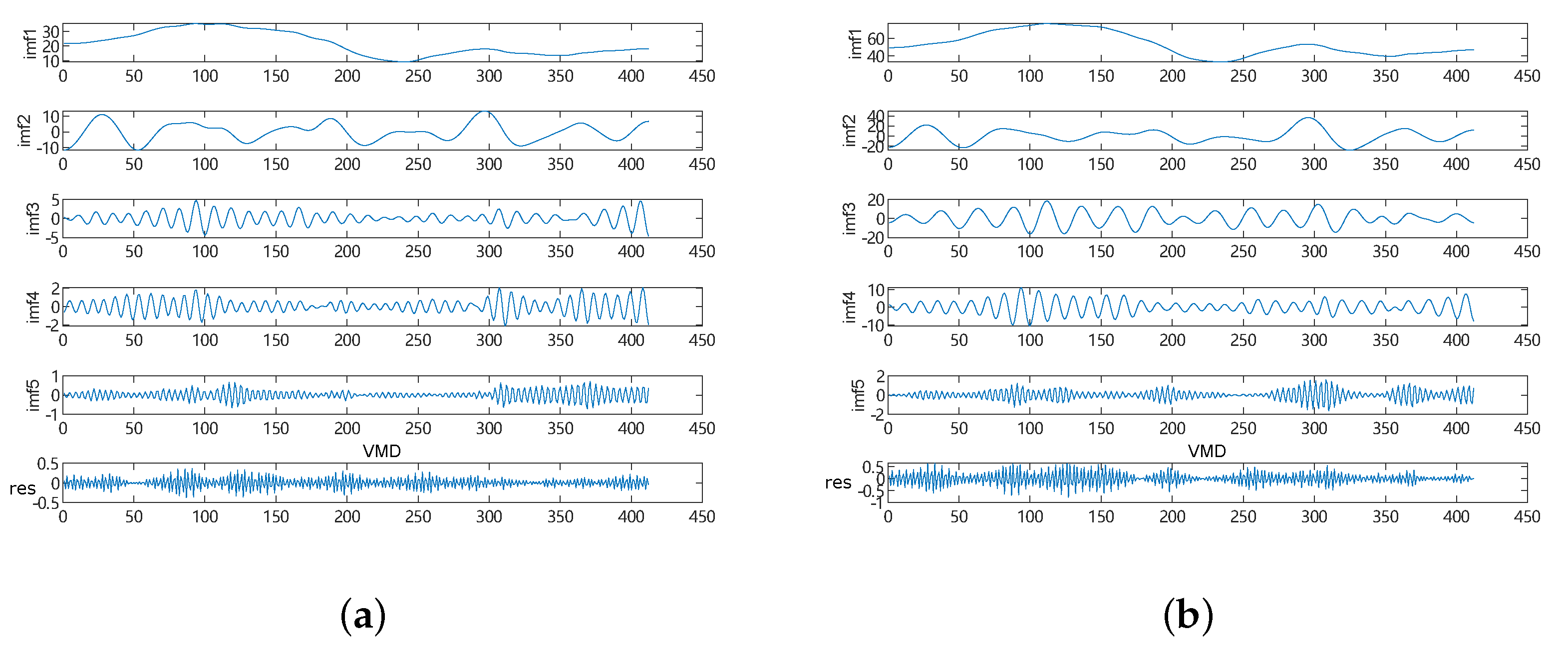
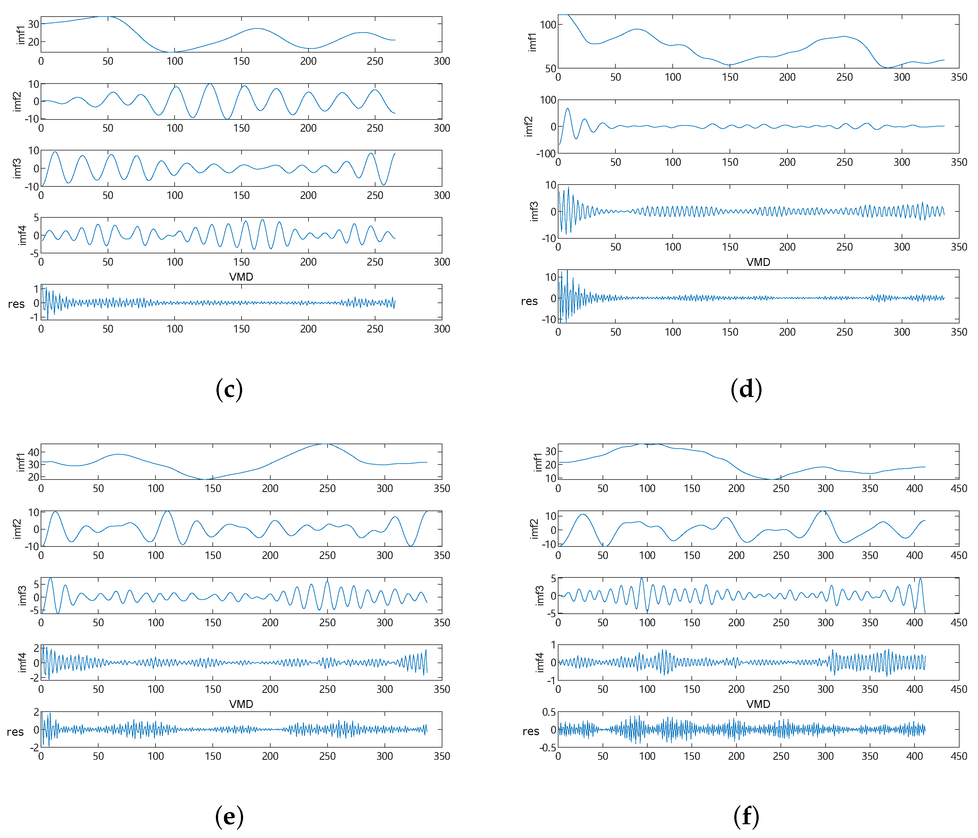
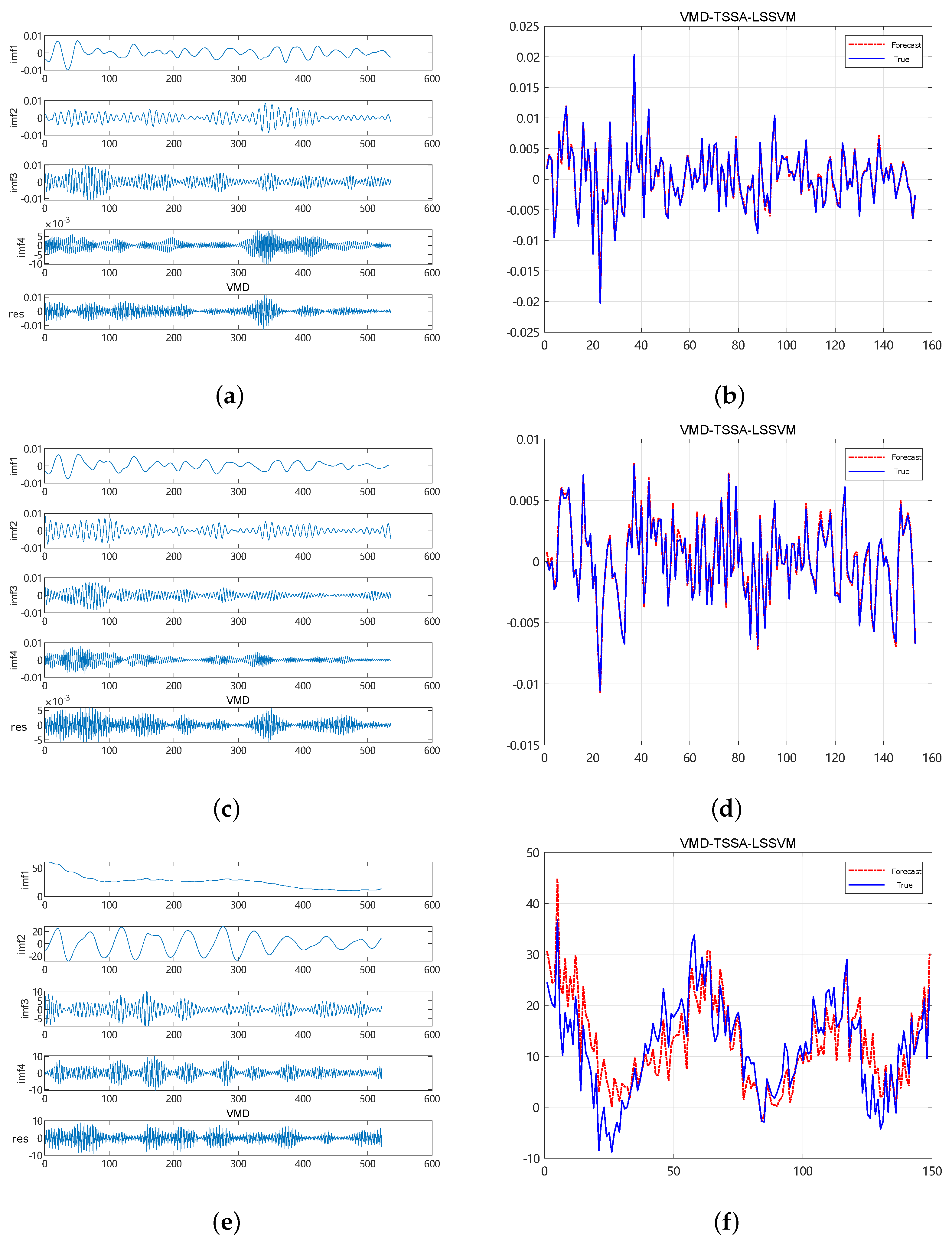
Inspired by the reference [26,27,28], considering the non-linearity and non-stationarity of ${\mathrm{PM}}_{2.5}$ and ${\mathrm{PM}}_{10}$ data, which are the main pollutants affecting air quality, we introduce VMD and decompose the time series data of ${\mathrm{PM}}_{2.5}$ and ${\mathrm{PM}}_{10}$. 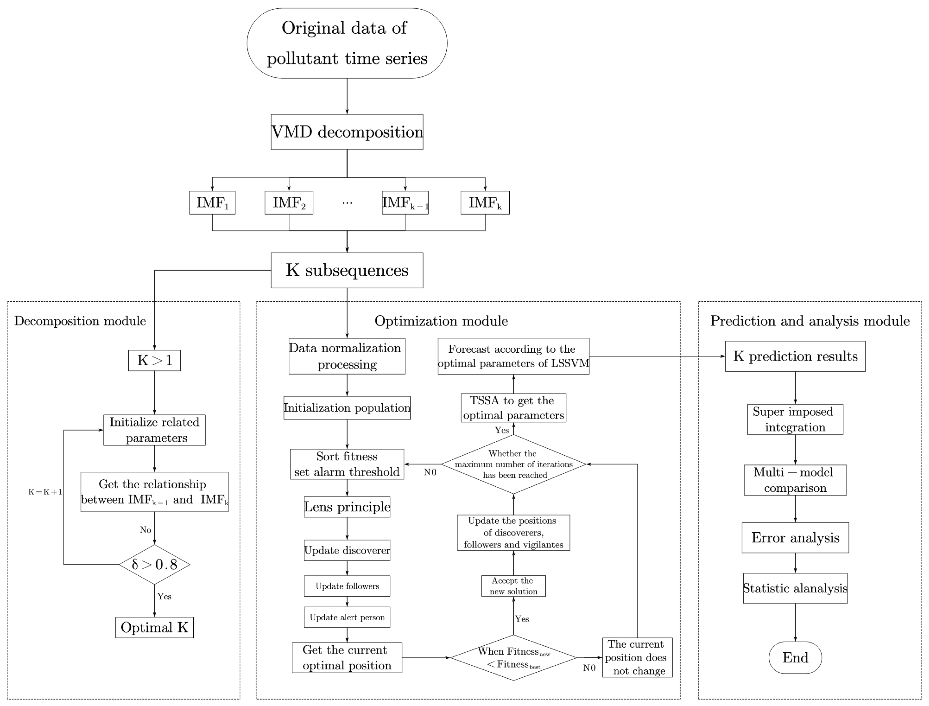At the same time, in order to improve the performance of SSA-LSSVM, we introduce the reverse learning strategy-lens principle [23] to optimize two important parameters of LSSVM, and establish a new model (TSSA-LSSVM) to further overcome the sensitivity of the least squares support vector machine to parameter selection.

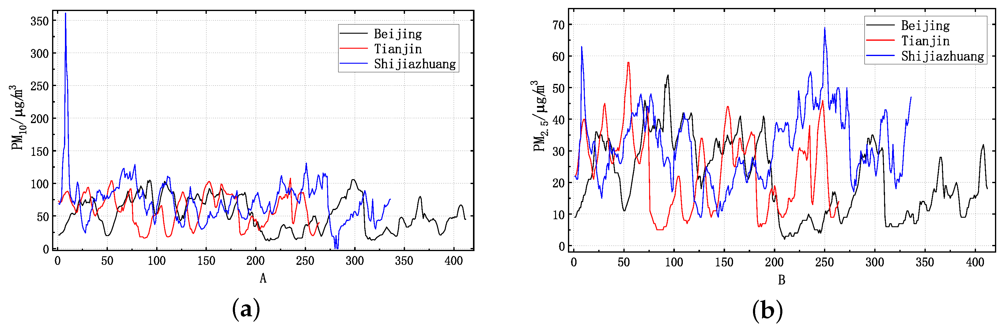
The main purpose of this paper is to improve the short-term pollutant prediction accuracy of cities in the Beijing–Tianjin–Hebei region by proposing a new hybrid model (VMD-TSSA-LSSVM) based on VMD and the machine learning method. And the major aims are as follows:

(1)

To deal with the instability and randomness of the original data of the ${\mathrm{PM}}_{2.5}$ and ${\mathrm{PM}}_{10}$ time series, the VMD technique is used to decompose the original signal into multiple modes to ensure the accuracy of the decomposed signal and avoid redundancies and over-decomposition.

(2)

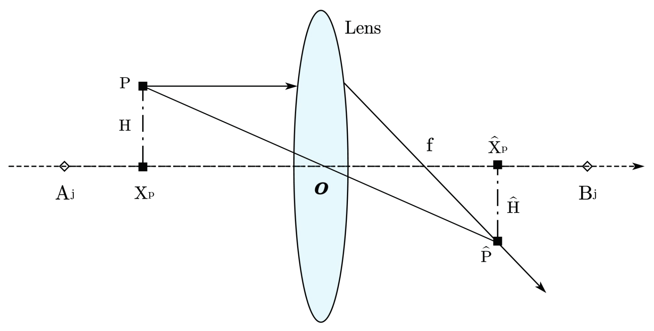
The lens principle is introduced to optimize the sparrow search algorithm, the SSA shows excellent performance in algorithm convergence and global optimization and the TSSA will further improve the performance of the optimized least squares support vector machine and obtain the optimal parameters.

(3)

To obtain effective prediction results and improve its practical application value, in the experimental stage, not only the excellent performance of the model is verified on the UCI data set, but the prediction results are also analyzed under multi-input and compared with other models to verify that the prediction accuracy of this model is better and more suitable for pollutant concentration prediction.

(4)

Finally, based on the experimental part, we carry out a statistical analysis to further verify the effectiveness of the model.

The rest of this article is organized as follows. In Section 2, some related work is reviewed. In Section 3, the main model is established and the relevant experimental analysis is carried out. Finally, in Section 6, we give the conclusion of this paper.

2. Related Work

2.1. Variational Mode Decomposition

Variational mode decomposition (VMD) is a new completely non-recursive, adaptive and quasi-orthogonal signal decomposition model [29,30] proposed by Dragomiretski and Zosso in 2014. The main purpose of VMD is to decompose the original signal by constructing and solving the following constrained variational problems to obtain a specified number of intrinsic mode function (IMF) components.

$$\left\{\begin{array}{c}\underset{(\left\{{\mu }_k\right\},\left\{{\omega }_k\right\})}{min}\{\sum _k\parallel {\partial }_t[(\delta \left(t\right)+\frac{j}{\pi t})\times {\mu }_k\left(t\right)]e^{-j{\omega }_{k}t}{\parallel }_2^2\},\hfill \\ s.t.\sum _k{\mu }_k=f.\hfill \end{array}\right.$$

(1)

where $\left\{{\mu }_k\right\}=\{{\mu }_1,{\mu }_2,\dots {\mu }_k\}$ and $\left\{{\omega }_k\right\}=\{{\omega }_1,{\omega }_2,\dots {\omega }_k\}$ represent the frequency centers of k mode components and each component, respectively. $\partial \left(t\right)$ is the partial derivative of time t, and j is the imaginary unit. Further, ${\mu }_k\left(t\right)$ and ${\omega }_k\left(t\right)$ are represented as:

$${\mu }_k\left(t\right)=A_k\left(t\right)cos{\psi }_k\left(t\right).$$

(2)

$${\omega }_k\left(t\right)={\psi }_k^{\prime }\left(t\right)=\frac{d{\psi }_k}{dt}.$$

(3)

where $A_k\left(t\right)$ is the amplitude of ${\mu }_k\left(t\right)$ when the time is t. In order to transform the constrained variational problem into an unconstrained problem, we introduce the Lagrange multiplier $\lambda$ and penalty factor $\beta$. Therefore, Equation (1) can be rewritten as:

$$\begin{array}{ccc}\hfill L\{{\omega }_k\left(t\right)·{\mu }_k\left(t\right),\lambda \}& =& \beta \sum _k{\parallel {\alpha }_t[(\delta \left(t\right)+\frac{j}{\pi t})\times {\mu }_k\left(t\right)]e^{-j{\omega }_{k}t}\parallel }_2^2\hfill \\ & +& \parallel f-\sum _k{\mu }_k{\left(t\right)\parallel }_2^2+⟨\lambda \left(t\right),f-\sum _k\left(t\right)⟩.\hfill \end{array}$$

(4)

Therefor, based on the literature [30], the Lagrange equation Equation (4) can be easily solved in the Fourier domain, as follows:

$${\tilde{\mu }}_k^{n+1}\left(\omega \right)=\frac{\tilde{f}\left(\omega \right)-{\sum }_{i\ne k}{\tilde{\mu }}_i\left(\omega \right)+\frac{\tilde{\lambda }\left(\omega \right)}{2}}{1+2\beta {(\omega -{\omega }_k)}^2}.$$

(5)

$${\omega }_k^{n+1}=\frac{{\int }_0^{\infty }\omega {\left|\tilde{\mu }\left(\omega \right)\right|}^{2}d\omega }{{\int }_0^{\infty }{\left|\tilde{\mu }\left(\omega \right)\right|}^{2}d\omega }.$$

(6)

$${\tilde{\lambda }}^{n+1}\left(\omega \right)={\tilde{\lambda }}^n\left(\omega \right)+\sigma (\tilde{f}\left(\omega \right)-\sum _k{\mu }_i^{n+1}\left(\omega \right)).$$

(7)

where the real component $\tilde{k}\left(t\right)$ can be obtained by an inverse fourier transformation, ${\omega }_k^{n+1}$ is the central frequency of the corresponding modal function and n is the number of iterations. The original input sequence to be decomposed is introduced into the variational model through the VMD algorithm, and each component is obtained by searching the optimal solution of the constrained variational model. In this process, each component adaptively decomposes the frequency band of the signal and updates alternately in the frequency domain until the K narrowband components are finally obtained. How to determine the effective decomposition number will directly affect the result of the IMF decomposition. The central frequency method can directly determine the decomposition scale K by using the central frequency value obtained by VMD, so the central frequency method has been widely used.

2.2. Sparrow Search Algorithm

The sparrow search algorithm (SSA) is a new type of group optimization algorithm proposed by Xue and Shen [22]. In nature, the sparrow is a gregarious animal with a clear division of labor. The predation process of the sparrow can be abstracted as a discoverer–participator model, and the reconnaissance and early warning mechanism is considered. The discoverer actively seeks the food source, while the participator monitors and obtains the food through the discoverer. Create a sparrow population in a dimensional search space, and the location of each sparrow is as follows:

$$X=\left[\begin{array}{ccc}{x}_{1,1}& \cdots & x_{1,D}\\ x_{2,1}& \cdots & x_{2,D}\\ ⋮& ⋮& ⋮\\ x_{N,1}& \cdots & x_{N,D}\end{array}\right]$$

(8)

where N denotes the number of sparrows and D represents the dimension of the variable to be optimized. Further, the fitness values of all sparrows can be expressed by the following vectors:

$$F_X=\left[\begin{array}{ccc}f(x_{1,1}& \cdots & x_{1,D})\\ f(x_{2,1}& \cdots & x_{2,D})\\ ⋮& ⋮& ⋮\\ f(x_{N,1}& \cdots & x_{N,D})\end{array}\right]$$

(9)

The value of each row in $f\left(x\right)$ represents the fitness value of the individual. In the SSA, the discoverer with a better adaptive value gives priority to food and guides the flow of the whole flock during the search. During each iteration, the position change expression of the discoverer is as follows:

$$X_{i,j}^{t+1}=\left\{\begin{array}{c}{X}_{i,j}^t·exp\left(\frac{-i}{\gamma ·I_{max}}\right),R_2<S,\hfill \\ X_{i,j}^t+Q·L,R_2\ge S.\hfill \end{array}\right.$$

(10)

In Equation (10), $j=(1,2,\dots ,D)$, t represents the current number of iterations, and $X_{i,j}^t$ denotes the position information of the ith Sparrow in the j dimension. $I_{max}$ is the constant with the maximum number of iterations. $\gamma (\gamma \in (0,1\left]\right)$ is a random number, and $R_2(R_2\in [0,1])$ and $S(S\in [0.5,1.0\left]\right)$ represent the alarm value and the safety threshold, respectively. Q is a random number with a normal distribution. L denotes that each element is the $1\times D$ dimensional matrix of 1.

For the participants, they will not only follow the participants to find food, but also constantly monitor them to compete for food to improve their predation rate. If there are starving participants, they will fly to other places to find food to obtain a higher fitness. The position change expression of the participant is as follows:

$$X_{i,j}^{t+1}=\left\{\begin{array}{c}Q·exp\left(\frac{X_{worst}^t-X_{i,j}^t}{i^2}\right),i>\frac{N}{2},\hfill \\ X_p^{t+1}+|X_{i,j}^t-X_p^{t+1}|·A^{*}·L,else.\hfill \end{array}\right.$$

(11)

In Equation (11), $X_p$ is the best position occupied by the producer. $X_{worst}$ is currently the worst location globally. $A^{*}=A^T{\left(A{A}^T\right)}^{-1}$ is a $1\times D$ dimension matrix, and each element is 1 or −1. Further, we assume that the initial position of the early warning sparrow is randomly generated in the population, and the position change expression of the early warning is as follows:

$$X_{i,j}^{t+1}=\left\{\begin{array}{c}{X}_{best}^t+\theta ·|X_{i,j}^t-X_{best}^t|,f_i>f_g,\hfill \\ X_{i,j}^t+K\left(\frac{|X_{i,j}^t-X_{worst}^t|}{f_i-f_w+\epsilon }\right),f_i=f_g.\hfill \end{array}\right.$$

(12)

In Equation (12), $K(K\in [-1,1\left]\right)$ is a random number. $\epsilon$ takes the lowest constant to avoid a denominator of 0. $X_{best}$ is currently the best location globally. $\theta$ is a parameter that controls the step size, and it is a normal distribution of random numbers with a mean of 0 and a variance of 1. $f_i$ is the current adaptation value of sparrows. $f_g$ and $f_w$ are the best and worst global fitness values, respectively.

2.3. Opposition-Based Learning Strategy Based on the Lens Principle

Suppose there is an individual with a height of H in a dimensional space, and the projection of the individual on the x axis is $\widehat{P}$, and $\widehat{P}$ is the new individual generated by the reverse learning strategy based on the principle of lens imaging. The schematic is as follows:

In Figure 1, the focal length is F, and O is not only the location point of the individual, but also the midpoint of the upper and lower limit $[A_j,B_j]$ of the current individual in the j dimension. The corresponding point of $X_P$ is ${\widehat{X}}_P$; we can then obtain:

$$\frac{\frac{(A+B)}{2}-X_P}{{\widehat{X}}_P-\frac{(A+B)}{2}}=\frac{H}{\widehat{H}}.$$

(13)

Figure 1. Lens schematic diagram.

Let $\frac{H}{\widehat{H}}=k$ represent the scale factor; we can obtain:

$${\widehat{X}}_P=\frac{A+B}{2}+\frac{A+B}{2k}-\frac{X_P}{k}.$$

(14)

We extend Equation (14) to the n dimensional space:

$${\widehat{X}}_P^j=\frac{A_j+B_j}{2}+\frac{A_j+B_j}{2k}-\frac{X_P^j}{k}.$$

(15)

where ${\widehat{X}}_P^j$ and $X_P^j$ represent the j dimension variables of ${\widehat{X}}_P$ and $X_P$, respectively.

2.4. Least Squares Support Vector Machine (LSSVM)

The least squares support vector machine (LSSVM) [31], as an improvement of the support vector machine (SVM) [32], simplifies a large quadratic programming (QP) problem to a set of smaller QP problems, and transforms the inequality constraint problem in the SVM into an equality constraint problem, thus reducing the difficulty of solving.

In the training sample set $T=\left\{(x_i,y_i)\right|x_i\in {\mathbb{R}}^n,y_i\in \mathbb{R},i=1,2,\dots ,N\}$, $x_i$ represents the k input vector, and $y_i$ represents the corresponding output value. N is the number of training samples. The model of the LSSVM in the feature space is expressed as

$$y={\omega }^T\phi \left(x\right)+b.$$

(16)

where $\phi \left(x\right)$ is the nonlinear mapping function, $\omega$ is the weight vector in the feature space and b is the offset. The LSSVM regression is based on the principle of structural risk minimization, and its expression is as follows:

$$R=\frac{1}{2}{\parallel \omega \parallel }^2+C·R_{emp}.$$

(17)

where ${\parallel \omega \parallel }^2$ represents model complexity, C represents regularization parameters and empirical risk function is represented by $R_{emp}$. Combined with the formulas Equations (16) and (17), the objective function of LSSVM is

$$\begin{array}{c}\hfill minJ(\omega ,\xi )=\frac{1}{2}{\parallel \omega \parallel }^2+C\sum _{i=1}^N{\xi }_i^2,\\ \hfill s.t{y}_i={\omega }^T\phi \left(x\right)+b+{\xi }_i.\end{array}$$

(18)

where ${\xi }_i$ represents the error variable. Further, the Lagrange multiplier method is used to solve the Equation (18); the Lagrange equation is defined as follows:

$$\begin{array}{c}\hfill L(\omega ,b,\xi ,\alpha )=J(\omega ,\xi )-\sum _{i=1}^N{\alpha }_i[{\omega }^T\phi \left(x\right)+b+{\xi }_i-y_i].\end{array}$$

(19)

where ${\alpha }_i\in R$ is the Lagrange multiplier. Through the KKT (Karush–Khun–Tucker) condition, we obtain the partial derivative of $\omega ,b,\xi ,\alpha$ and make it zero.

$$\left\{\begin{array}{c}\frac{\partial L}{\partial \omega }=0\to \omega ={\Sigma }_{i=1}^N{\alpha }_i\phi \left(x_i\right),\hfill \\ \frac{\partial L}{\partial b}=0\to {\Sigma }_{i=1}^N{\alpha }_i=0,\hfill \\ \frac{\partial L}{\partial {\xi }_i}=0\to {\alpha }_i=C·{\xi }_i,\hfill \\ \frac{\partial L}{\partial {\alpha }_i}=0\to {\omega }^T\phi \left(x_i\right)+b+{\xi }_i-y_i=0.\hfill \end{array}\right.$$

(20)

The optimization problem can be transformed into a linear equation by Equation (20), by eliminating $\omega$ and ${\xi }_i$, where the following matrix equation can be obtained.

$$\left[\begin{array}{cc}0& I_N^T\\ I_N& \mathsf{\Omega }+C^{-1}I\end{array}\right]\left[\begin{array}{c}b\\ \alpha \end{array}\right]=\left[\begin{array}{c}0\\ y\end{array}\right]$$

(21)

where $y={[y_1,y_2,\dots ,y_N]}^T$, $I_N\in R^N$, I is a unit matrix, and ${\mathsf{\Omega }}_{i,j}={\varphi }^T\left(x_i\right)\varphi \left(x_j\right)$ is a kernel function. Through the Mercer condition, there is a mapping $\phi$ and a kernel function $K\left(x\right)$; we can obtain:

$$\begin{array}{c}\hfill K(x_i,x_j)={\phi }^T\left(x_i\right)\phi \left(x_j\right).\end{array}$$

(22)

Therefore, the optimal linear regression function of the LSSVM is:

$$\begin{array}{c}\hfill f{\left(x_i\right)}_j=\sum _{i=1}^N\sum _{j=1}^N{\alpha }_{i,j}K(x_i,x_j)+b_j.\end{array}$$

(23)

In this paper, the radial basis function (RBF) is chosen as the sum function of the least square support vector machine, because the RBF can map samples to a high-dimensional space and has a strong learning ability, less constraints and good local approximation characteristics; the expression is as follows:

$$\begin{array}{c}\hfill K(x_i,x_j)=exp(-\frac{\parallel x_x-y_i{\parallel }^2}{{\sigma }^2}).\end{array}$$

(24)

where ${\sigma }^2$ is the kernel parameter.

3. Methodology

3.1. Our Method

First of all, the structure flow chart of this model is given intuitively in Figure 2, and its main contribution is:

Figure 2. VMD-TSSA-LSSVM algorithm framework.

(a)

Data processing and decomposition: Combined with VMD, the target data is decomposed to obtain the set component $IM{F}_1,IM{F}_2,\cdots ,IM{F}_K$.

(b)

Integrated prediction: The K components are predicted by VMD-TSSA-LSSVM and the final target value is obtained by adding the results, and the prediction accuracy is considered.

(c)

Experimental analysis: Based on the UCI data set and the pollutant data set of the Beijing–Tianjin–Hebei region, the prediction results of this model are verified.

(d)

Comparison and verification: Compared with other models, five error indexes are used to analyze its performance. At the same time, a reasonable statistical analysis is given.

3.2. Data Description

In order to verify the validity and reliability of the proposed method in the application of time series data, in this part of the experiment, we select three sets of time series data sets, including ${\mathrm{HCC}}_{\mathrm{EM}}$ and ${\mathrm{HCC}}_{\mathrm{EU}}$ (Hungarian Chickenpox Cases: a spatio-temporal dataset of weekly chickenpox (childhood disease) cases from Hungary. The dataset consists of a county-level adjacency matrix and time series of the county-level reported cases between 2005 and 2015. There are two specific related tasks: county level case count prediction and nation level case count prediction), and the ISE (ISTANBUL STOCK EXCHANGE: Stock exchange returns. The Istanbul stock exchange national 100 index, Standard and poors 500 return index, Stock market return index of Germany, Stock market return index of UK, Stock market return index of Japan, Stock market return index of Brazil, MSCI European index, MSCI emerging markets index) are from the UCI database (https://archive.ics.uci.edu/ml/index.php (accessed on 27 July 2022)). The details are described in Table 1. In the three datasets, 70% of the original data is selected as the training set and 30% as the test set.

Table 1. UCI dataset description.

	HCCEM	HCCEU	ISE
Data Characteristics	Time-Series	Time-Series	Multivaritate, Time-Series
Data scale	$536\times 20$	$536\times 20$	$522\times 8$
Associated Tasks	Regression	Regression	Classification, Regression

The data used in this paper comes from the national air quality online monitoring platform (https://air.cnemc.cn:18007/ (accessed on 27 July 2022)). The platform converts the main detection values of pollutants into alphanumeric form. In addition to the predicted respirable particulate matter ${\mathrm{PM}}_{2.5}$ and ${\mathrm{PM}}_{10}$, there are also ${\mathrm{SO}}_2$, ${\mathrm{NO}}_2$, ${\mathrm{O}}_3$ and CO. In addition, much literature shows that meteorological factors also affect air quality, so we also consider temperature, humidity, wind speed and wind level. See Table 2 for details.

Table 2. Variable description.

Variable	Unit	Variable	Unit	Variable	Unit	Variable	Unit
${\mathrm{PM}}_{2.5}$	$\mathsf{\mu }$g/m${}^3$	$\mathrm{CO}$	mg/m${}^3$	$\mathrm{Temperature}$	${}^{\circ }$C	${\mathrm{NO}}_2$	$\mathsf{\mu }$g/m${}^3$
${\mathrm{PM}}_{10}$	$\mathsf{\mu }$g/m${}^3$	${\mathrm{SO}}_2$	$\mathsf{\mu }$g/m${}^3$	$\mathrm{Humidity}$	$NA$	$\mathrm{Wind}\mathrm{speed}$	m/s
${\mathrm{O}}_3$	$\mathsf{\mu }$g/m${}^3$	$\mathrm{Wind}\mathrm{level}$	m/s

4. Experimental Analysis

4.1. Analysis and Results of the UCI Dataset

4.1.1. VMD Decomposition and Prediction Result

In the first step, in the process of decomposing the target data set using the VMD, the main parameters that affect the decomposition result are the determination of penalty factor $\alpha$ and the number of decomposition layers K. Based on relevant theories and many experiments [23,26,27], the range of the penalty factor is selected in the range of 3000 to 8000 for the collected data in this paper. This is because the penalty factor is about the narrower the bandwidth of the component signal is. This will further affect the final signal sequence processing results.

In the second step, for the K value, because the distribution of the center frequency of the ${\mu }_K$ components obtained by the VMD processing is from low to high, we choose the K value from small to large during the experiment. When the center frequency of the last layer of the ${\mu }_K$ components reaches the maximum and the region is stable, the K value is determined to be optimal. Based on the above, the K on three UCI datasets is 5. The specific decomposition results are shown in Figure 3.

Figure 3. Decomposition and prediction based on UCI data. Res denotes Residual; the center frequency value corresponding to each IMF (imf) component can be obtained by VMD; X-axis denotes Number of time periods (weeks). (a) $HC{C}_{EM}$ decomposition; (b) $HC{C}_{EM}$ Forecast; (c) $HC{C}_{EU}$ decomposition; (d) $HC{C}_{EU}$ Forecast; (e) $ISE$ decomposition; (f) $ISE$ Forecast.

In the third step, the parameters of TSSA optimization LSSVM are selected as follows: the initial sparrow individual is a, the number of discoverers accounts for 15% of the total population and the maximum number of iterations is set to 50. The parameter range of the LSSVM is set to $[{10}^{-6},400]$, and in order to prevent the parameter from being zero, we set the minimum value of the range parameter to ${10}^{-7}$, which is close to zero but not zero, to prevent the prediction result from being inaccurate.

In the fourth step, we use Equation (25), which is commonly used in machine learning, to obtain the prediction accuracy of the data set on the model in this paper. The details are as follows:

$$ACC=1-\frac{|{\widehat{x}}_i-x_i|}{{\widehat{x}}_i}\times 100\%.$$

(25)

where ACC indicates the accuracy of prediction, and $x_i$ and ${\widehat{x}}_i$ represent the real value and predicted value, respectively.

We can directly observe from Figure 3 that the prediction results of VMD-TSSA-LSSVM on ${\mathrm{HCC}}_{\mathrm{EM}}$ and ${\mathrm{HCC}}_{\mathrm{EU}}$ reach a very ideal state, and the prediction accuracy is 99.79% and 99.17%, respectively, which fully shows that the prediction effect of this model can achieve the expected results on UCI data sets whose data characteristics are only time series. Similarly, in order to fully compare and comprehensively consider, we also select the multivariable dataset-ISE, which can be used for classification, and its prediction result is 80.31%, and the accuracy also meets the basic prediction requirements. At the same time, we can see from the chart that the prediction curve accords with the trend of the original curve, which shows that the model in this paper is feasible on the UCI dataset.

4.1.2. Error Index and Analysis

To ensure a comprehensive inspection and evaluation of the model, this paper selects five different error indicators to avoid the misleading caused by a single result. That is, the MSE (Means Quare Error), RMSE (Root Means Quare Error), MAE (Mean Absolute Error), MAPE (Mean Absolute Percentage Error) and SMAPE (Symmetric Mean Absolute Percentage Error) to evaluate the effect of the model are defined as follows:

$$\begin{array}{ccc}\hfill MSE& =& \frac{1}{N}{\Sigma }_{i=1}^N{({\widehat{x}}_i-x_i)}^2.\hfill \end{array}$$

(26)

$$\begin{array}{ccc}\hfill RMSE& =& \sqrt{\frac{1}{N}{\Sigma }_{i=1}^N{({\widehat{x}}_i-x_i)}^2}.\hfill \end{array}$$

(27)

$$\begin{array}{ccc}\hfill MAE& =& \frac{1}{N}{\Sigma }_{i=1}^N|{\widehat{x}}_i-x_i|.\hfill \end{array}$$

(28)

$$\begin{array}{ccc}\hfill MAPE& =& \frac{1}{N}{\Sigma }_{i=1}^N\left|\frac{{\widehat{x}}_i-x_i}{x_i}\right|\times 100\%.\hfill \end{array}$$

(29)

$$\begin{array}{ccc}\hfill SMAPE& =& \frac{1}{N}{\Sigma }_{i=1}^N\frac{|{\widehat{x}}_i-x_i|}{\left(\right|{\widehat{x}}_i|+|x_i\left|\right)/2}\times 100\%.\hfill \end{array}$$

(30)

where N is the number of each dataset, and $x_i$ and ${\widehat{x}}_i$ represent the real value and predicted value of the input variable, respectively. The smaller the value, the smaller the error. The commonly used $R^2$ (R-Squared) is not considered here because the limitation of the data will cause its denominator to be zero.

In Table 3, we show the MSE, RMSE, MAPE, SMAPE and MAE analysis results of VMD-TSSA-LSSVM under three UCI datasets. It is well known that the smaller the error value based on statistical learning theory, the higher the accuracy of the model. As can be seen from Table 2, the method proposed in this paper achieves better results in five kinds of error analyses. The error results of ${\mathrm{HCC}}_{\mathrm{EM}}$, ISE and ${\mathrm{HCC}}_{\mathrm{EU}}$ also correspond with the prediction accuracy, which further shows the excellent performance of VMD-TSSA-LSSVM in predicting time series data.

Table 3. MSE, RMSE, MAPE, SMAPE and MAE analysis results of VMD-TSSA-LSSVM under three UCI datasets.

Index	HCCEM	HCCEU	ISE	Index	HCCEM	HCCEU	ISE
MSE	$1.39\times {10}^{-7}$	$1.19\times {10}^{-7}$	28.44	MAPE (%)	0.24	1.42	25.60
RMSE	$3.72\times {10}^{-4}$	$3.46\times {10}^{-4}$	5.33	SMAPE (%)	3.77	4.57	17.36
MAE	$2.99\times {10}^{-4}$	$2.82\times {10}^{-4}$	4.42

4.2. Practical Application and Comparison

The study area is the Beijing–Tianjin–Hebei region, which mainly selected Beijing (northern latitude ${39}^{\circ }{26}^{\prime }$–${40}^{\circ }{15}^{\prime }$, east longitude ${115}^{\circ }{25}^{\prime }$–${117}^{\circ }{30}^{\prime }$), Tianjin (northern latitude ${38}^{\circ }{33}^{\prime }$–${41}^{\circ }{03}^{\prime }$, east longitude ${116}^{\circ }{42}^{\prime }$–${118}^{\circ }{04}^{\prime }$) and Shijiazhuang (northern latitude ${37}^{\circ }{27}^{\prime }$–${38}^{\circ }{47}^{\prime }$, east longitude ${113}^{\circ }{30}^{\prime }$–${115}^{\circ }{20}^{\prime }$), the capital of Hebei Province, as this study. There are 38, 24 and 51 monitoring points in the three cities. According to the same interval and different time span in different periods, the data are obtained hour by hour. There are 1015 data in total, as shown in Table 4.

Table 4. Data information.

	Datasets
	Beijing	Tianjin	Shijiazhuang
Data size	412 h	264 h	336 h
Data type	hourly	hourly	hourly
Training set	13:00 16 May 2022∼13:00 28 May 2022	00:00 22 May 2022∼15:00 29 May 2022	12:00 31 May 2022∼07:00 10 June 2022
Test set	14:00 28 May 2022∼16:00 2 June 2022	16:00 29 May 2022∼23:00 1 June 2022	08:00 10 June 2022∼11:00 14 June 2022
Predicted target	${\mathrm{PM}}_{2.5}$; ${\mathrm{PM}}_{10}$	${\mathrm{PM}}_{2.5}$; ${\mathrm{PM}}_{10}$	${\mathrm{PM}}_{2.5}$; ${\mathrm{PM}}_{10}$
Average value	21.54; 53.46	23.53; 60.03	31.46; 72.72
Data range	2–54; 12–106	5–58; 16–108	9–69; 0–361

Furthermore, the time series data of ${\mathrm{PM}}_{10}$ and ${\mathrm{PM}}_{2.5}$ of Beijing, Tianjin and Shijiazhuang are visually shown in Figure 4. Among them, a few missing points are completed by average interpolation.

Figure 4. ${\mathrm{PM}}_{10}$ and ${\mathrm{PM}}_{2.5}$ under three datasets. X-axis denotes Number of time periods (weeks). (a) ${\mathrm{PM}}_{10}$ time series data; (b) ${\mathrm{PM}}_{2.5}$ time series data.

Experiment and Comparison

In this section, we first give the VMD decomposition results of six datasets: Beijing PM${}_{10}$ (BPM${}_{10}$), Beijing PM${}_{2.5}$ (BPM${}_{2.5}$), Tianjin PM${}_{10}$ (TPM${}_{10}$), Tianjin PM${}_{2.5}$ (TPM${}_{2.5}$), Shijiazhuang PM${}_{10}$ (TPM${}_{10}$) and Shijiazhuang PM${}_{2.5}$ (TPM${}_{2.5}$). The range of K values is 4–6, as shown in Figure 5.

Figure 5. Decompositio of six groups of pollutant data. Res denotes Residual; the center frequency value corresponding to each IMF (imf) component can be obtained by VMD; X-axis denotes Number of time periods (weeks). (a) ${\mathrm{BPM}}_{10}$; (b) ${\mathrm{BPM}}_{2.5}$; (c) ${\mathrm{TPM}}_{10}$; (d) ${\mathrm{TPM}}_{2.5}$; (e) ${\mathrm{SPM}}_{10}$; (f) ${\mathrm{SPM}}_{2.5}$.

After verifying the excellent performance of this model on UCI data sets, we consider not only the prediction performance of the Beijing–Tianjin–Hebei region on VMD-TSSA-LSSVM, but also back the propagation neural network (BPNN), least square support vector machine (LSSVM), classical particle swarm optimization (PSO-LSSVM) and VMD-LSSVM, SSA-LSSVM, TSSA-LSSVM related to this model. As can be seen from Figure 6, compared with the actual value, all models can obtain the approximate trend, among which the prediction curve of VMD-TSSA-LSSVM is the most close to the actual value; especially on the data set ${\mathrm{BPM}}_{10}$ and ${\mathrm{BPM}}_{2.5}$, the prediction accuracy is $96.72\%$ and $98.79\%$, respectively.

Figure 6. Prediction results of pollutant data under seven models. X-axis denotes Number of time periods (weeks). (a) ${\mathrm{BPM}}_{10}$; (b) ${\mathrm{BPM}}_{2.5}$; (c) ${\mathrm{TPM}}_{10}$; (d) ${\mathrm{TPM}}_{2.5}$; (e) ${\mathrm{SPM}}_{10}$; (f) ${\mathrm{SPM}}_{2.5}$.

The results of each data under five kinds of error evaluations are shown in Table 5. Among them, the smaller the value is, the better the prediction performance is. We bold the best predictives as black in each group of data. It can be seen from the table that the performance of VMD-TSSA-LSSVM is the best compared with the other six models. In particular, there is a difference of between VMD-TSSA-LSSVM and PSO-LSSVM under MSE, RMSE, MAE, MAPE, SMAPE. It is obvious that its prediction performance has been greatly improved. At the same time, the prediction accuracy of VMD-LSSVM and TSSA-LSSVM is similar, which shows that it is meaningful for us to use the lens principle to optimize the sparrow algorithm. At the same time, the VMD method can decompose and reconstruct time series data, obtain models with high stability, high efficiency and learning speed and help VMD-TSSA-LSSVM get rid of the disadvantage of autocorrelation.

Table 5. Comparison of error results.

Case		BPNN	LSSVM	PSO-LSSVM	SSA-LSSVM	VMD-LSSVM	TSSA-LSSVM	VMD-TSSA-LSSVM
MSE	${\mathrm{BPM}}_{10}$	17.27	5.71	3.40	2.55	2.02	2.04	$\mathbf{0}.\mathbf{85}$
	${\mathrm{BPM}}_{2.5}$	79.70	24.98	11.81	9.83	5.74	5.50	$\mathbf{4}.\mathbf{46}$
	${\mathrm{TPM}}_{10}$	36.93	9.32	8.15	7.04	5.12	5.01	$\mathbf{3}.\mathbf{72}$
	${\mathrm{TPM}}_{2.5}$	99.12	43.68	34.01	31.45	25.19	25.76	$\mathbf{7}.\mathbf{05}$
	${\mathrm{SPM}}_{10}$	62.28	33.45	32.61	24.05	21.53	18.38	$\mathbf{2}.\mathbf{73}$
	${\mathrm{SPM}}_{2.5}$	99.98	84.31	79.88	74.89	70.02	67.88	$\mathbf{9}.\mathbf{29}$
RMSE	${\mathrm{BPM}}_{10}$	4.16	2.39	1.84	1.60	1.42	1.43	$\mathbf{0}.\mathbf{92}$
	${\mathrm{BPM}}_{2.5}$	8.93	4.50	3.44	3.14	2.40	2.34	$\mathbf{2}.\mathbf{11}$
	${\mathrm{TPM}}_{10}$	6.08	3.05	2.86	2.65	2.26	2.24	$\mathbf{1}.\mathbf{93}$
	${\mathrm{TPM}}_{2.5}$	9.99	6.61	5.83	5.61	5.02	5.08	$\mathbf{2}.\mathbf{66}$
	${\mathrm{SPM}}_{10}$	7.89	5.78	5.71	4.90	4.64	4.29	$\mathbf{1}.\mathbf{65}$
	${\mathrm{SPM}}_{2.5}$	9.96	9.18	8.94	8.65	8.37	8.24	$\mathbf{3}.\mathbf{05}$
MAE	${\mathrm{BPM}}_{10}$	3.01	1.94	1.45	1.29	1.14	1.15	$\mathbf{0}.\mathbf{77}$
	${\mathrm{BPM}}_{2.5}$	6.59	3.95	2.92	2.72	2.05	2.01	$\mathbf{1}.\mathbf{74}$
	${\mathrm{TPM}}_{10}$	4.99	2.44	2.29	2.18	1.72	1.72	$\mathbf{1}.\mathbf{64}$
	${\mathrm{TPM}}_{2.5}$	7.53	5.75	4.89	4.81	4.17	4.25	$\mathbf{1}.\mathbf{93}$
	${\mathrm{SPM}}_{10}$	6.51	4.67	4.73	4.05	3.90	3.51	$\mathbf{1}.\mathbf{38}$
	${\mathrm{SPM}}_{2.5}$	7.59	7.18	7.07	7.31	7.07	6.98	$\mathbf{2}.\mathbf{29}$
MAPE $(\%)$	${\mathrm{BPM}}_{10}$	13.63	9.31	6.97	7.06	6.15	6.11	$\mathbf{4}.\mathbf{28}$
	${\mathrm{BPM}}_{2.5}$	10.96	8.18	5.35	4.90	3.97	3.85	$\mathbf{2}.\mathbf{86}$
	${\mathrm{TPM}}_{10}$	20.62	11.67	10.66	9.86	8.60	8.53	$\mathbf{7}.\mathbf{46}$
	${\mathrm{TPM}}_{2.5}$	13.04	10.22	8.60	8.51	7.40	7.54	$\mathbf{2}.\mathbf{69}$
	${\mathrm{SPM}}_{10}$	15.04	10.90	11.12	9.65	9.50	8.70	$\mathbf{3}.\mathbf{72}$
	${\mathrm{SPM}}_{2.5}$	13.23	7.56	7.43	9.35	9.40	9.28	$\mathbf{2}.\mathbf{98}$
SMAPE $(\%)$	${\mathrm{BPM}}_{10}$	9.25	6.13	4.59	4.68	4.09	4.06	$\mathbf{2}.\mathbf{86}$
	${\mathrm{BPM}}_{2.5}$	7.40	5.52	3.40	3.29	2.66	2.58	$\mathbf{1}.\mathbf{90}$
	${\mathrm{TPM}}_{10}$	14.39	7.87	7.19	6.64	5.74	5.69	$\mathbf{4}.\mathbf{98}$
	${\mathrm{TPM}}_{2.5}$	8.86	6.83	5.77	5.71	4.96	5.05	$\mathbf{1}.\mathbf{80}$
	${\mathrm{SPM}}_{10}$	10.17	7.34	7.47	6.48	6.33	5.79	$\mathbf{2}.\mathbf{48}$
	${\mathrm{SPM}}_{2.5}$	9.21	5.24	5.14	6.22	6.23	6.15	$\mathbf{1}.\mathbf{99}$

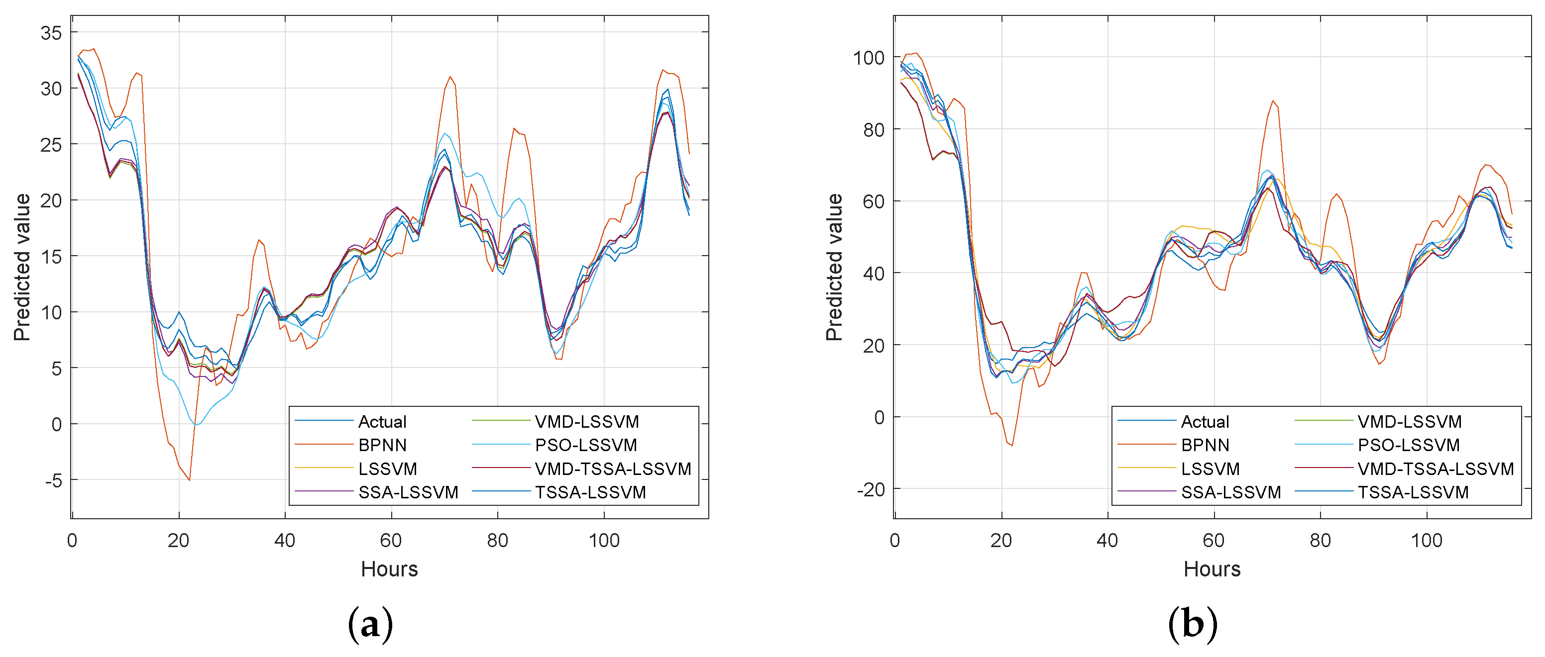
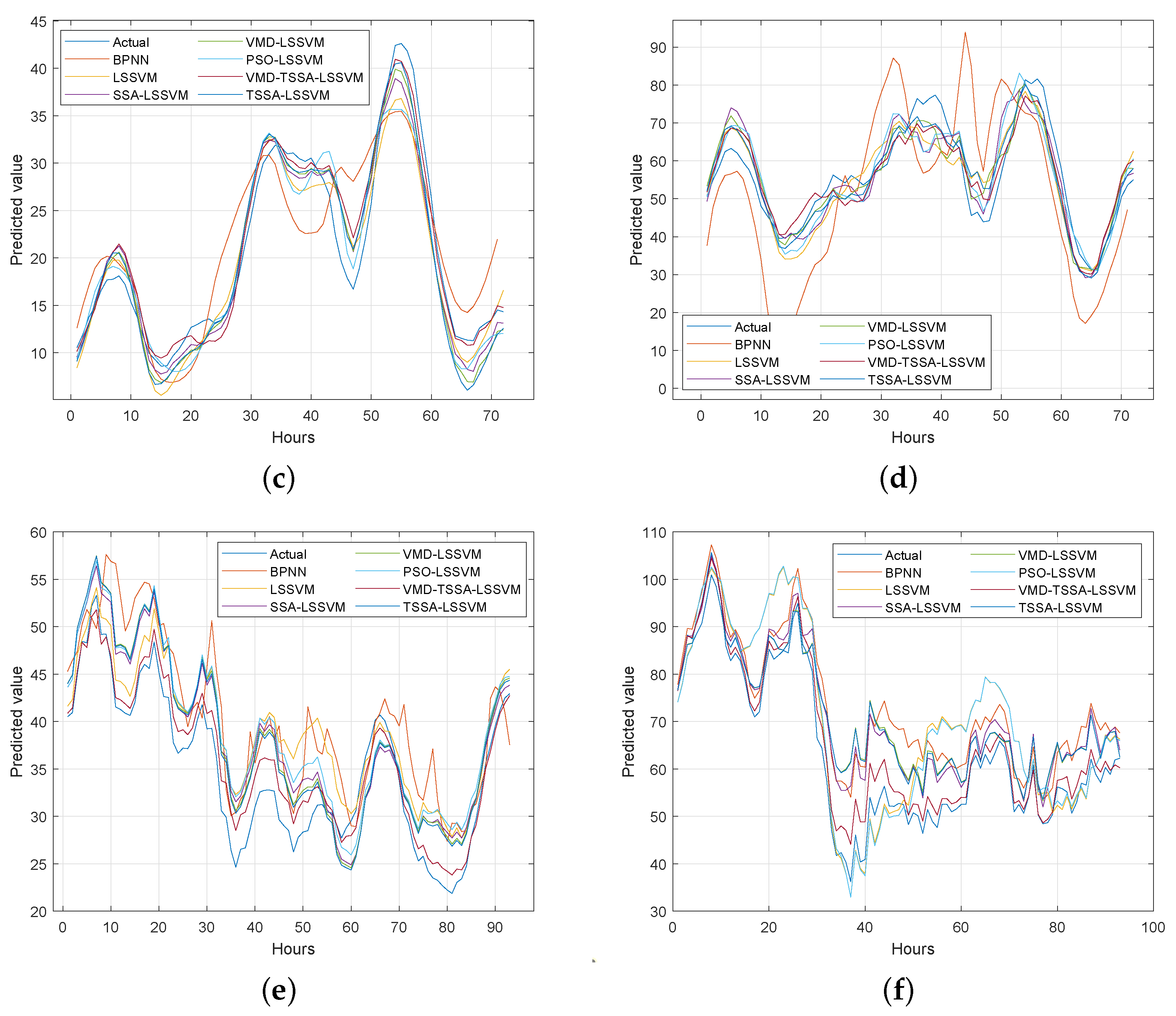
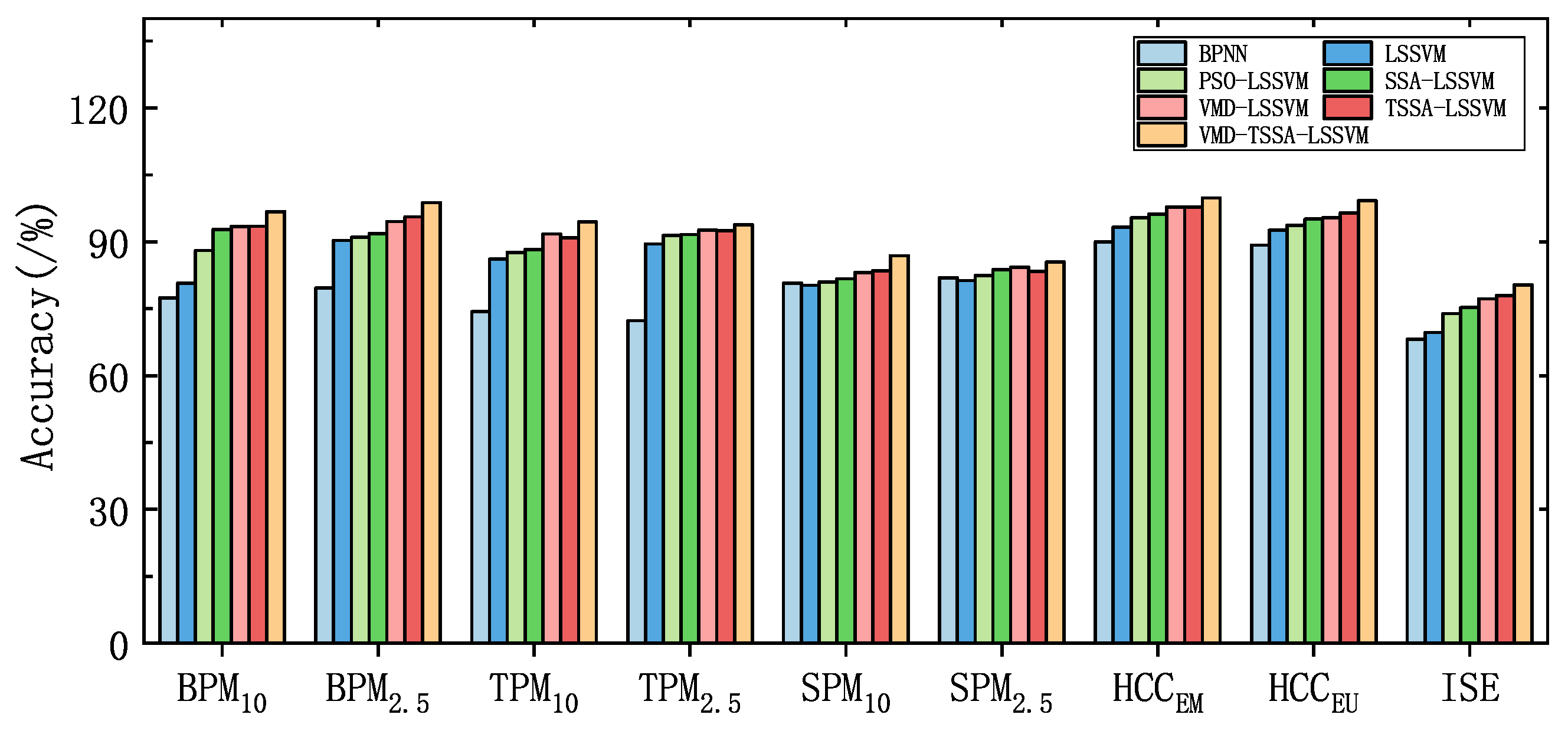
5. Statistical Analysis

In this section, we want to use the famous Friedman test [33] to analyze the differences between the seven models on the UCI data set and the pollutant data set. The Friedman test is chosen because it can make full use of the information of the original data and has the advantages of a safe and reliable nonparametric test. First of all, the prediction accuracy of the seven models on nine datasets is visually shown in Table 6 and Figure 7. It can be seen from the chart that the prediction accuracy of VMD-TSSA-LSSVM is higher.

Table 6. Summary of prediction accuracy for all datasets.

	BPNN	LSSVM	PSO-LSSVM	SSA-LSSVM	VMD-LSSVM	TSSA-LSSVM	VMD-TSSA-LSSVM
Datasets	$ACC(\%)$	$ACC(\%)$	$ACC(\%)$	$ACC(\%)$	$ACC(\%)$	$ACC(\%)$	$ACC(\%)$
${\mathrm{BPM}}_{10}$	77.36	80.72	88.04	92.81	93.43	93.46	96.72
${\mathrm{BPM}}_{2.5}$	79.58	90.28	91.00	91.77	94.51	94.55	98.79
${\mathrm{TPM}}_{10}$	74.32	86.12	87.61	88.28	91.70	90.91	94.45
${\mathrm{TPM}}_{2.5}$	72.79	89.47	91.40	91.57	92.61	92.47	93.85
${\mathrm{SPM}}_{10}$	80.76	80.23	81.02	81.71	83.10	83.52	86.86
${\mathrm{SPM}}_{2.5}$	81.89	81.26	82.38	83.70	84.25	83.37	85.47
$HC{C}_{EM}$	90.01	93.27	95.38	96.19	97.82	97.74	99.79
$HC{C}_{EU}$	89.23	92.54	93.66	95.05	95.33	96.48	99.17
ISE	68.11	69.62	73.91	75.24	77.18	77.94	80.31

Figure 7. Prediction accuracy.

Next, to facilitate the statistical analysis, Table 7 shows the average ranking and accuracy of all models on nine data sets. It can be seen from Table 7 that the accuracy of this model is 13.48%, 7.99%, 5.66%, 4.34%, 2.83% and 2.77% higher than that of BPNN, LSSVM, PSO-LSSVM, SSA-LSSVM, VMD-LSSVM and TSSA-LSSVM, respectively. And it is higher in the rankings.

Table 7. Average accuracy and ranking.

	BPNN	LSSVM	PSO-LSSVM	SSA-LSSVM	VMD-LSSVM	TSSA-LSSVM	TSSA-LSSVM
Avg.ACC	79.34	84.83	87.16	88.48	89.99	90.05	92.82
Avg.rank	6.78	6.22	5	3.89	2.56	2.56	1

The formula for Friedman statistical variables is as follows:

$${\chi }_F^2=\frac{12N}{k(k+1)}[\sum _i{R}_i^2-\frac{k{(k+1)}^2}{4}]=51.87.$$

(31)

where k is the number of algorithms in this paper, and N is the number of selected data sets, including UCI data sets and pollutant data sets. In this paper, the values of k and N are 7 and 9, respectively, and $R_i$ represents the average ranking of seven algorithms.

In addition, according to the ${\chi }_F^2$ distribution with $k-1$ degrees of freedom, we can obtain:

$$F_F=\frac{(N-1){\chi }_F^2}{N(k-1)-{\chi }_F^2}=194.82.$$

(32)

where $F_F((k-1),(k-1)(N-1))$ obeys the F-distribution, and its degree of freedom is $(k-1)$ and $(k-1)(N-1)$. In this paper, we choose $\alpha =0.1$ and we can obtain $F_{\alpha }(6,48)=1.90$. Obviously, $F_F$ is much larger than $F_{\alpha }$, so we reject the zero hypothesis.

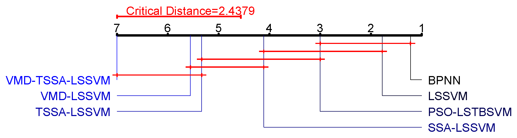
Next, through the Nemenyipost-hoctest, we can further compare the errors of the seven algorithms in this paper. Comparing the average rank difference with the critical value, the greater the numerical difference is, the more obvious the difference in algorithm performance is. Therefore, we use the following formula to calculate the critical difference (CD) and obtain $q_{\alpha }=2.394$.

$$CD=q_{\alpha =0.05}\times \sqrt{\frac{k(k+1)}{6N}}=2.4379.$$

(33)

To better analyze the advantages of the method presented in this paper, we visualized the statistical analysis results in Figure 8. We see that VMD-TSSA-LSSVM has significant statistical differences compared to BPNN, LSSVM, PSO-LSSVM and SSA-LSSVM, and thus our method is better than these four algorithms, because the difference between them is less than the CD value. Furthermore, we can observe that there is no significant difference between VMD-TSSA-LSSVM and TSSA-LSSVM, VMD-LSSVM, as the difference is smaller than the CD value. Therefore, based on the statistical analysis, it is safe to conclude that the VMD-TSSA-LSSVM is performs better. This shows that the prediction performance of the new hybrid model based on TSSA-LSSVM and VMD-LSSVM has been further improved.

Figure 8. Visualization comparison of statistical analysis of seven methods.

6. Conclusions

The following is the summary and prospect of this study.

• Selecting the VMD method to decompose non-stationary time series data, including UCI data and pollutant data, can effectively reduce the complexity of original data, eliminate autocorrelation, reduce the number of non-stationary features and abrupt changes and obtain more regular sub-series. By constantly adjusting the size of the set K value to avoid incomplete decomposition and over-decomposition, this operation can reduce the computational cost and eliminate frequency overlap. In future research, we can use some novel time series methods (such as phase space reconstruction (PSR), energy entropy (EE), etc.) to obtain the optimal K value.
• In this paper, the important parameters of the LSSVM are optimized by the TSSA. The results show that the TSSA is better than the SSA. This is because the lens principle can optimize the current solution and projection solution at the same time, and obtain a better solution. However, based on machine learning, there are still many methods (such as the extreme learning machine (ELM) and deep learning (DL)) that can be used in pollutant problems, and more optimization algorithms are worth exploring, not limited to heuristic algorithms.
• By comparing the results of the proposed model with the results of BPNN, LSSVM, PSO-LSSVM, VMD-LSSVM, SSA-LSSVM and TSSA-LSSVM models, it is verified that higher prediction accuracy can be obtained in either the UCI data set or the Beijing–Tianjin–Hebei region pollutant data set. The results of nine data sets are 96.72%, 94.45%, 93.85%, 86.86%, 85.47%, 99.79%, 99.17% and 80.31%, respectively. At the same time, MSE, RMSE, MAE, MAPE and SMAPE are used to evaluate the performance of the model. VMD-TSSA-LSSVM is superior to other models. Therefore, the proposed hybrid model can be used as a tool to predict the concentration of pollutants.

References

1. Bollen, J. The value of air pollution co-benefits of climate policies: Analysis with a global sector-trade CGE model called WorldScan. Technol. Forecast. Soc. Chang. 2015, 90, 178–191. [Google Scholar] [CrossRef]
2. Wu, L.; Li, N.; Yang, Y. Prediction of air quality indicators for the Beijing-Tianjin-Hebei region. J. Clean. Prod. 2018, 196, 682–687. [Google Scholar] [CrossRef]
3. Zheng, S.; Singh, R.P.; Wu, Y.; Wu, C. A comparison of trace gases and particulate matter over Beijing (China) and Delhi (India). Water Air Soil Pollut. 2017, 228, 1–15. [Google Scholar] [CrossRef]
4. Bouazza, N.; Foissac, F.; Urien, S.; Guedj, R.; Carbajal, R.; Tréluyer, J.M.; Chappuy, H. Fine particulate pollution and asthma exacerbations. Arch. Dis. Child. 2018, 103, 828–831. [Google Scholar] [CrossRef]
5. Gu, S.; Wu, S.; Yang, L.; Hu, Y.; Tian, B.; Yu, Y.; Ma, N.; Ji, P.; Zhang, B. Synoptic Weather Patterns and Atmospheric Circulation Types of PM2.5 Pollution Periods in the Beijing-Tianjin-Hebei Region. Atmosphere 2023, 14, 942. [Google Scholar] [CrossRef]
6. Geng, G.; Zhang, Q.; Martin, R.V.; van Donkelaar, A.; Huo, H.; Che, H.; Lin, J.; He, K. Estimating long-term PM2.5 concentrations in China using satellite-based aerosol optical depth and a chemical transport model. Remote Sens. Environ. 2015, 166, 262–270. [Google Scholar] [CrossRef]
7. Jeong, J.I.; Park, R.J.; Woo, J.H.; Han, Y.J.; Yi, S.M. Source contributions to carbonaceous aerosol concentrations in Korea. Atmos. Environ. 2011, 45, 1116–1125. [Google Scholar] [CrossRef]
8. Tie, X.; Brasseur, G.P.; Zhao, C.; Granier, C.; Massie, S.; Qin, Y.; Wang, P.; Wang, G.; Yang, P.; Richter, A.; et al. Chemical characterization of air pollution in Eastern China and the Eastern United States. Atmos. Environ. 2006, 40, 2607–2625. [Google Scholar] [CrossRef]
9. Berkowicz, R.; Palmgren, F.; Hertel, O.; Vignati, E. Using measurements of air pollution in streets for evaluation of urban air quality-meterological analysis and model calculations. Sci. Total Environ. 1996, 189, 259–265. [Google Scholar] [CrossRef]
10. Byun, D.; Schere, K.L. Review of the governing equations, computational algorithms, and other components of the Models-3 Community Multiscale Air Quality (CMAQ) modeling system. Appl. Mech. Rev. 2006, 59, 51–77. [Google Scholar] [CrossRef]
11. Kumar, A.; Goyal, P. Forecasting of air quality in Delhi using principal component regression technique. Atmos. Pollut. Res. 2011, 2, 436–444. [Google Scholar] [CrossRef]
12. Sun, W.; Sun, J. Daily PM2.5 concentration prediction based on principal component analysis and LSSVM optimized by cuckoo search algorithm. J. Environ. Manag. 2017, 188, 144–152. [Google Scholar] [CrossRef]
13. Hong, W.C. Application of chaotic ant swarm optimization in electric load forecasting. Energy Policy 2010, 38, 5830–5839. [Google Scholar] [CrossRef]
14. Zhang, L.; Lin, J.; Qiu, R.; Hu, X.; Zhang, H.; Chen, Q.; Tan, H.; Lin, D.; Wang, J. Trend analysis and forecast of PM2.5 in Fuzhou, China using the ARIMA model. Ecol. Indic. 2018, 95, 702–710. [Google Scholar] [CrossRef]
15. Rahman, N.H.A.; Lee, M.H.; Latif, M.T. Artificial neural networks and fuzzy time series forecasting: An application to air quality. Qual. Quant. 2015, 49, 2633–2647. [Google Scholar] [CrossRef]
16. Bai, Y.; Li, Y.; Wang, X.; Xie, J.; Li, C. Air pollutants concentrations forecasting using back propagation neural network based on wavelet decomposition with meteorological conditions. Atmos. Pollut. Res. 2016, 7, 557–566. [Google Scholar] [CrossRef]
17. Russo, A.; Lind, P.G.; Raischel, F.; Trigo, R.; Mendes, M. Neural network forecast of daily pollution concentration using optimal meteorological data at synoptic and local scales. Atmos. Pollut. Res. 2015, 6, 540–549. [Google Scholar] [CrossRef]
18. Mogollón-Sotelo, C.; Casallas, A.; Vidal, S.; Celis, N.; Ferro, C.; Belalcazar, L. A support vector machine model to forecast ground-level PM2.5 in a highly populated city with a complex terrain. Air Qual. Atmos. Health 2021, 14, 399–409. [Google Scholar] [CrossRef]
19. Garg, H. A hybrid GA-GSA algorithm for optimizing the performance of an industrial system by utilizing uncertain data. In Handbook of Research on Artificial Intelligence Techniques and Algorithms; IGI Global: Hershey, PA, USA, 2015; pp. 620–654. [Google Scholar]
20. Dongxiao, N.; Tiannan, M.; Bingyi, L. Power load forecasting by wavelet least squares support vector machine with improved fruit fly optimization algorithm. J. Comb. Optim. 2017, 33, 1122–1143. [Google Scholar] [CrossRef]
21. Garg, H. A hybrid GSA-GA algorithm for constrained optimization problems. Inf. Sci. 2019, 478, 499–523. [Google Scholar] [CrossRef]
22. Xue, J.; Shen, B. A novel swarm intelligence optimization approach: Sparrow search algorithm. Syst. Sci. Control Eng. 2020, 8, 22–34. [Google Scholar] [CrossRef]
23. Song, C.; Yao, L.; Hua, C.; Ni, Q. A water quality prediction model based on variational mode decomposition and the least squares support vector machine optimized by the sparrow search algorithm (VMD-SSA-LSSVM) of the Yangtze River, China. Environ. Monit. Assess. 2021, 193, 1–17. [Google Scholar] [CrossRef] [PubMed]
24. Chen, H.; Duan, J.; Yin, R.; Ponkratov, V.V.; Guerrero, J.W.G. Prediction of penetration rate by Coupled Simulated Annealing-Least Square Support Vector Machine (CSA-LSSVM) learning in a hydrocarbon formation based on drilling parameters. Energy Rep. 2021, 7, 3971–3978. [Google Scholar] [CrossRef]
25. Sun, J.; Zhang, H.; Li, Q.; Liu, H.; Lu, X.; Hou, K. Contamination degree prediction of insulator surface based on exploratory factor analysis-least square support vector machine combined model. High Volt. 2021, 6, 264–277. [Google Scholar] [CrossRef]
26. Chu, J.; Dong, Y.; Han, X.; Xie, J.; Xu, X.; Xie, G. Short-term prediction of urban PM2.5 based on a hybrid modified variational mode decomposition and support vector regression model. Environ. Sci. Pollut. Res. 2021, 28, 56–72. [Google Scholar] [CrossRef]
27. Chen, S.; Wang, J.; Zhang, H. A hybrid PSO-SVM model based on clustering algorithm for short-term atmospheric pollutant concentration forecasting. Technol. Forecast. Soc. Chang. 2019, 146, 41–54. [Google Scholar] [CrossRef]
28. Ouyang, C.; Zhu, D.; Wang, F. A learning sparrow search algorithm. Comput. Intell. Neurosci. 2021, 2021, 3946958. [Google Scholar] [CrossRef] [PubMed]
29. Dragomiretskiy, K.; Zosso, D. Variational mode decomposition. IEEE Trans. Signal Process. 2013, 62, 531–544. [Google Scholar] [CrossRef]
30. Kumar, A.; Gandhi, C.P.; Zhou, Y.; Kumar, R.; Xiang, J. Variational mode decomposition based symmetric single valued neutrosophic cross entropy measure for the identification of bearing defects in a centrifugal pump. Appl. Acoust. 2020, 165, 107294. [Google Scholar] [CrossRef]
31. Cortes, C.; Vapnik, V. Support-vector networks. Mach. Learn. 1995, 20, 273–297. [Google Scholar] [CrossRef]
32. Suykens, J.A.; Vandewalle, J. Least squares support vector machine classifiers. Neural Process. Lett. 1999, 9, 293–300. [Google Scholar] [CrossRef]
33. Demar, J. Statistical comparisons of classifiers over multiple data sets. J. Mach. Learn. Res. 2006, 7, 1–3. [Google Scholar]
Disclaimer/Publisher’s Note: The statements, opinions and data contained in all publications are solely those of the individual author(s) and contributor(s) and not of MDPI and/or the editor(s). MDPI and/or the editor(s) disclaim responsibility for any injury to people or property resulting from any ideas, methods, instructions or products referred to in the content.
Article Metrics
Citations
Article Access Statistics
Multiple requests from the same IP address are counted as one view.