Error Analysis and Visibility Classification of Camera-Based Visiometer Using SVM under Nonstandard Conditions

Abstract

A camera-based visiometer is a promising atmospheric visibility measurement tool because it can meet some specific demands such as the need for visibility monitoring in a strong way, whereas traditional instruments, such as forward scatter-type sensors and transmissometers, can hardly be widely utilized due to their high cost. The camera-based method is used to measure visibility by recording the luminance contrast of the objects in an image. However, lacking standard conditions, they can hardly obtain absolute measurements even with blackbody objects. In this paper, the errors caused by nonstandard conditions in camera-based visiometers with two artificial black bodies are analyzed. The results show that the luminance contrasts of the two blackbodies are highly dependent on the environmental radiance distribution. The nonuniform sky illuminance can cause a large error in the blackbody contrast estimations, leading to substantial visibility measurement errors. A method based on a support vector machine (SVM) is proposed to classify the visibility under nonstandard conditions to ensure the reliability of the camera-based visiometer. A classification accuracy of 96.77% was achieved for the data containing images depicting different illumination conditions (e.g., a clear sky, cloudy sky, and overcast). The results show that the classifier based on the SVM is an effective and reliable method to estimate visibility under complex conditions.

1. Introduction

Atmospheric visibility plays an important role in transportation safety. The probability of traffic accidents dramatically increases under low visibility conditions. Many instrumentations have been developed to monitor atmospheric visibility, such as transmissometers [1], forward or backward scatter-type sensors [2], lidars [3], and image-based visiometers [4,5,6], and some of them have been widely used in the area of meteorology, transportation, and environment monitoring. Camera-based visibility sensors are potentially the optimal solution for reducing traffic accidents caused by low visibility conditions, because the existing Closed-circuit Television (CCTV) network can provide real-time traffic images to estimate the atmospheric visibility [7,8,9,10].

Atmospheric visibility can be calculated by using the atmospheric extinction coefficient, which is measured by using the luminance contrast of the objects in an image. Duntley [11] quantitatively derived the physical relationship between the apparent contrast and the atmospheric extinction coefficient in a homogenous atmosphere, which is also referred to as the standard condition. This approach was proven to be effective by many studies. The visibility was obtained by measuring the apparent contrast between black objects and an adjacent sky that was captured by using film cameras [12]. Compared to film cameras, video cameras can provide automatic successive visibility measurements with more accurate luminance information about the objects and background in images. Ishimoto et al. [13] developed a video-camera-based visibility measurement system with an artificial half-black and half-white plate used as a target, and the visibility that was measured by determining the contrast between the target and a standardized background highly agreed with transmissometer measurements under low visibility conditions. Based on contrast theory, Williams and Cogan [14] developed a new contrast calculation methodology in the spatial and frequency domain to estimate the equivalent atmospheric attenuation length to conduct visibility calculations from satellite images. In the frequency domain, the cloud contribution might be effectively filtered out by a high-pass filter. Barrios et al. [15] applied this approach to the visibility estimation with mountain images captured by an aircraft. By taking the visible mountains as primary landmarks, they obtained good visibility estimations with an approximate 20% error bound in high-visibility conditions. Du et al. [16] utilized two cameras at different distances to take photos of the same target, and the optical contrasts between a target and its sky background were calculated by using these two images to calculate the atmospheric visibility. He et al. [17] proposed a Dark Channel Prior (DCP) method to estimate the atmospheric transmission that is applied to estimate the visibility on the highway [18]. Atmospheric visibility can also be directly estimated without using Koschmieder’s theory. The edge information of the images is utilized to estimate the visibility with a regression model [19,20,21,22,23] or the predefined target location [7,24]. However, these two methods have not been widely adopted due to the absence of a universal regression model for the former method and the low precision of the latter method.

Due to the lack of absolute brightness references, the contrasts of the objects in an image captured by a video camera depends on their albedos and the environment illuminance [25]. Therefore, the contrast of the objects is not only a function of atmospheric visibility. As a result, many studies introduce artificial blackbodies in the system to establish an absolute brightness reference point in an image. With an artificial blackbody, the performance of the camera-based visiometer is significantly better than those with targets with a higher reflectivity [26], and the observations are consistent with the commercial visibility instruments used under low visibility conditions [27]. To eliminate the influence of the dark current and CCD gain of the video camera, double blackbodies have been adapted [4,5,6]. However, even with absolute brightness references such as artificial blackbodies, large errors in the camera-based visibility measurements have still been observed under high-visibility conditions [6]. The observed errors could be caused by an inhomogeneous atmosphere, in which Horvath [25] proved that the contrast-based visibility observations exhibit certain errors due to inhomogeneous illuminance. Allard and Tombach [28] found the dramatic effects of five nonstandard conditions caused by clouds or hazes upon conducting contrast-based visibility observations. Lu [29] numerically analyzed the visibility errors induced by the vertical relative gradients of sky luminance and nonuniform illumination along the sight path. However, excluding the effects of target reflectivity and systematic noise, the errors of nonstandard observation environments have not been systematically analyzed.

The essentials of the traditional camera-based visibility measurement methods are based on luminance contrasts of finite objects, which potentially lead to severe errors under nonstandard conditions. By extracting more information from numerous images, machine learning has been becoming a promising approach to classify the visibility in complex atmospheric environments. Varjo and Hannuksela [30] proposed an SVM model with the projections of the scene images to classify atmospheric visibility into five classes. Zhang et al. [31] recognized four levels of visibility with an optimal binary tree SVM by combining the contrast features in the specified regions and the transmittance features extracted by using the DCP method. Giyenko et al. [32] applied convolutional neural networks (CNN) to classify the visibility with a step of 1000 m, and their model achieved an accuracy of around 84% when using CCTV images. Lo et al. [33] established a multiple support vector regression model with an estimation accuracy above 90% regarding the visibilities in high-visibility conditions. You et al. [34] proposed a CNN-RNN (recurrent neural network) coarse-to-fine model to estimate the relative atmospheric visibility through deep learning by using massive pictures from the Internet. Additionally, multimethod fusion models have been studied. Yang et al. [35] proposed a fusion model to estimate visibilities with DCP, Weighted Image Entropy (WIE), and SVM. Wang et al. [36] proposed a CNN-based multimodal fusion network with visible–infrared image pairs. Machine learning and deep learning can provide a superior way to classify atmospheric visibility due to the reduced sensitivity to complex environmental illumination, but an acknowledged model that can be used to determine the absolute value estimation of visibility has not yet been proposed.

This paper explored the effect of nonstandard environmental illuminance on contrast-based visibility measurements by using visiometers with blackbodies. To mitigate the impact of nonstandard conditions, we proposed a supplementary method based on an SVM to classify the visibilities of images. This paper is organized as follows: in Section 2, the model that uses a semisimplified double-luminance contrast method is derived; in Section 3, three cases are employed to analyze the effect of environmental illuminance on visibility measurements with the luminance and cloud information; in Section 4, an algorithm based on an SVM is proposed; and Section 5 contains the conclusion.

2. Mathematical Model for Nonstandard Conditions

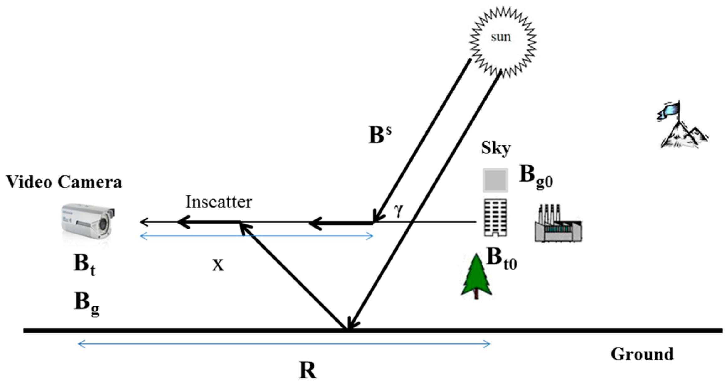
The visual range of a distant object is determined by the contrast of the object against the background, and the atmosphere extinction includes scattering and absorption along the line of sight from the object to the observer. The light reflected or emitted by the object undergoes intensity losses due to the scattering, absorption, and spectral shift caused by the aerosols and atmosphere molecules. The physical model of the light propagating from the objects to an observer is given in Figure 1.

In Figure 1, $B_{t0}$ is the radiance of the distant object located at $R$, and $B_t$ is the radiance of the object into the video camera. The relationship between $B_{t0}$ and $B_t$ is given by Equation (1):

$$B_t=B_{t0}{e}^{-\sigma R}+B_{IN}$$

(1)

where $\sigma$ is the atmosphere extinction coefficient and $R$ is the distance between the video camera and the object. $B_{IN}$ is the inscattering light as $B_{t0}$ propagates along the line from the object to the camera. The total light scattered into the viewing direction at the camera is shown in Equation (2):

$$B_{IN}={\displaystyle {\int }_0^R{e}^{-\sigma x}L\left(\gamma ,x\right)dx}$$

(2)

where $L\left(\gamma ,x\right)$ is the light scattered in direction $\gamma$ into the viewing direction of the camera at point $x$, and it is given by Equation (3):

$$L\left(\gamma ,x\right)={\displaystyle {\int }_0^{4\pi }{\displaystyle {\int }_{{\lambda }_l}^{{\lambda }_u}{B}^S\left({\gamma }^{\prime },\lambda ,x\right)\beta \left(\gamma ,{\gamma }^{\prime },\lambda ,x\right)d\lambda d{\gamma }^{\prime }}}$$

(3)

where $B^S\left(\lambda ,\gamma \right)$ represents the spectral radiance of the sun and sky in the direction $\gamma$ at wavelength $\lambda$, and the $\beta$ is the total scatter coefficient.

For the sky background $B_{g0}$ at location $R$, we can write the same format of the sky radiance at the camera, which is defined in Equation (4):

$$B_g=B_{g0}{e}^{-\sigma R}+B_{IN}$$

(4)

The relationship between the extinction coefficient and visibility is given by Koschmieder’s law, which is represented by Equation (5):

$$V=-\frac{\ln {\xi }_0}{\sigma }$$

(5)

where ${\xi }_0$ is the contrast ratio, which is recommended to be 0.02 by the World Meteorological Organization (WMO) or 0.05 by the International Civil Aviation Organization (ICAO).

By measuring the brightness of the target and sky background, the visibility can be calculated by Equation (6):

$$V=\frac{L\cdot \ln {\xi }_0}{\ln \left(1-\frac{B_t}{B_g}\right)-\ln \left(1-\frac{B_{t0}}{B_{g0}}\right)}$$

(6)

However, the intrinsic contrast cannot be obtained from the images due to the unknown variables $B_{t0}$ and $B_{g0}$. Therefore, blackbodies are introduced to avoid measuring an intrinsic contrast [26,27]. In addition, to eliminate the dark current of the camera, double blackbodies are adapted [4,6], and visibility can be obtained through Equation (7):

$$V=\frac{-(R_2-R_1)\ln {\xi }_0}{\ln \left(\frac{B_{t1}-B_g}{B_{t2}-B_g}\right)}$$

(7)

Even with double blackbody targets, Equation (7) is valid under standard conditions, which are:

(1)

The sky background is right behind the blackbodies in the image.

(2)

The homogenous distribution of inscattering light $B_{IN}$.

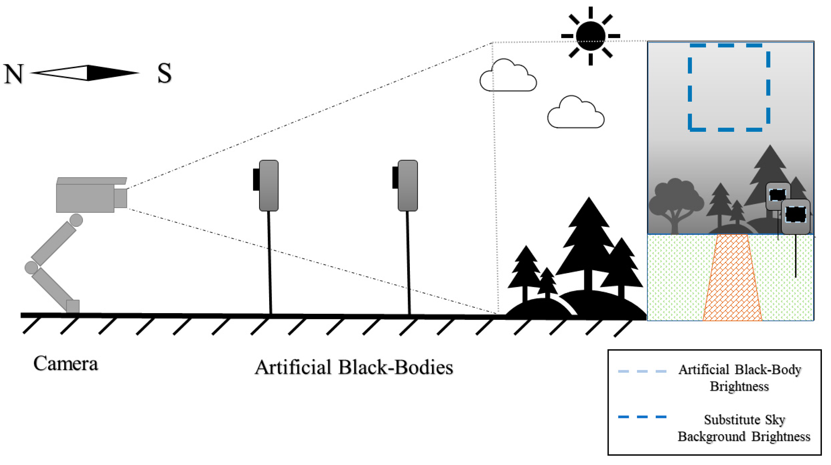
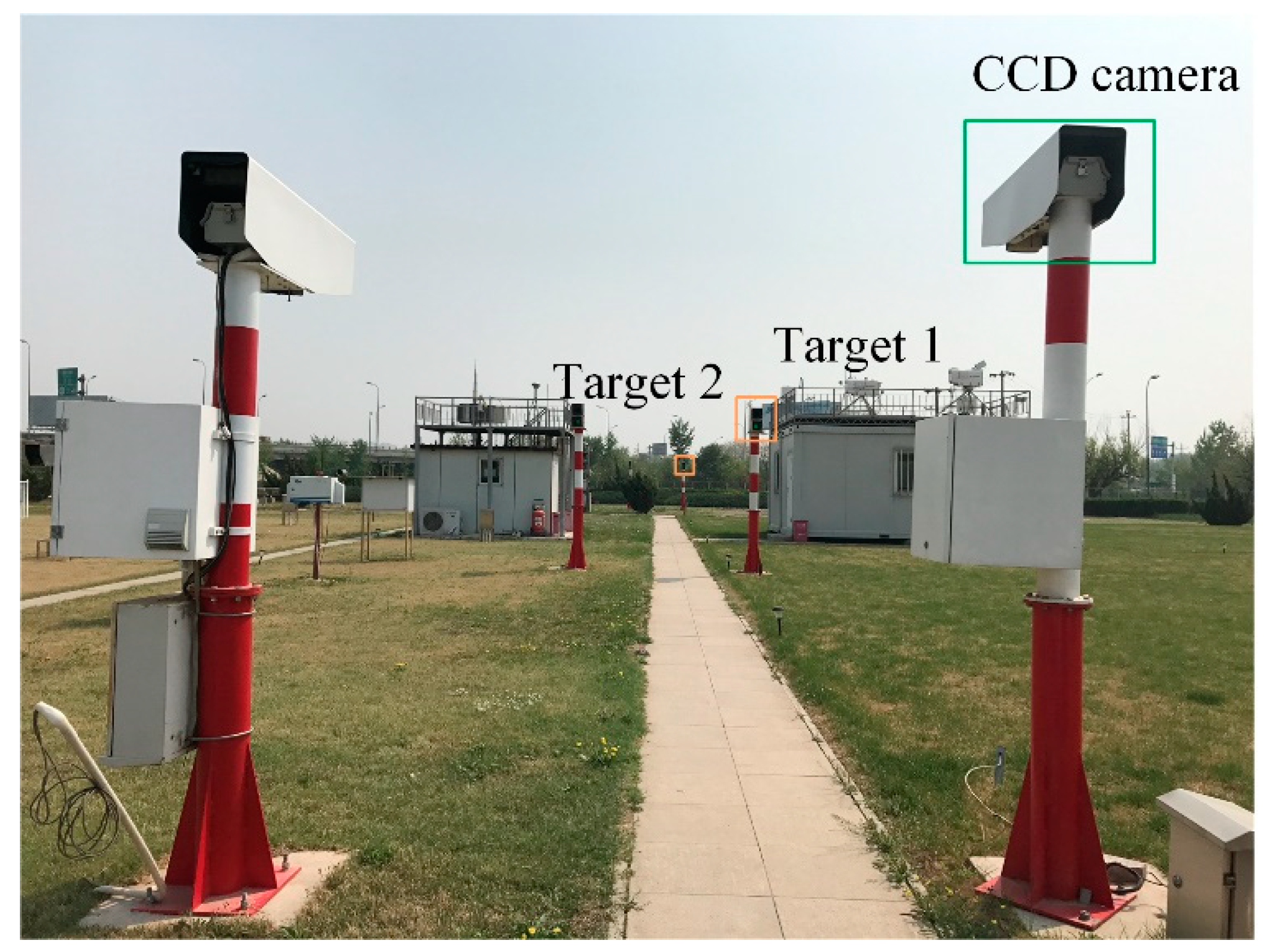
Usually, because of the obstruction of the mountains, buildings, or trees, the video camera cannot obtain the corresponding sky background luminance. As a substitute, another sky background, which has a different light path (usually a higher path) to the camera, is adopted to calculate the contrast, as shown in Figure 2. Because of clouds, plumes, the shadows of mountains, buildings, etc., $B^S\left(\lambda ,\gamma \right)$ can hardly be homogenous. As a result, the difference between the $B_{INt}$ of the target and $B_{INg}$ of the sky background is not net zero. So, the visibility equation under the nonstandard condition is expressed as Equation (8):

$$V=\frac{(R_1-R_2)\ln {\xi }_0}{\ln \left(\frac{B_{g1}-B_{t1}-\Delta B_{IN1}}{B_{g2}-B_{t2}-\Delta B_{IN2}}\right)-\ln \left(\frac{B_{g10}}{B_{g20}}\right)}$$

(8)

where $\Delta B_{INi}$ represents $B_{INgi}-B_{INti}$.

3. Results

For camera-based visiometers with double-targets systems or other systems [5,6,27], the intensities of the inscattering light between the targets and the camera and the brightness of the intrinsic sky background cannot be directly measured. Under the nonstandard conditions, the inhomogeneous inscattering light and nonstandard background would induce four additional unknown variables in the visibility calculation equation, as shown in Equation (8), and cause inevitable errors.

3.1. Error Analysis under Nonstandard Conditions

The total root mean square (RMS) visibility error is proportional to the true visibility values. Yu [6] proposed that the primary contributing factors to the error of DPVS are the CCD camera and nonideal blackbodies under standard conditions. However, the nonstandard conditions have an even more severe significant impact on the error of DPVS. For nonstandard conditions, the RMS for the visibility error is redefined as Equation (9):

$$\frac{\Delta V_{rms}}{V}=\frac{V}{(R_1-R_2)\ln {\xi }_0}{\left({\langle \Delta n_1/n_1\rangle }^2+{\langle \Delta n_2/n_2\rangle }^2+{\langle \Delta n_3/n_3\rangle }^2\right)}^{1/2}$$

(9)

where $n_1$, $n_2$, and $n_3$ represent $B_{g1}-B_{t1}-\Delta B_{IN1}$, $B_{g2}-B_{t2}-\Delta B_{IN2}$, and $\raisebox{1ex}{$B_{g10}$}\!\left/ \!\raisebox{-1ex}{$B_{g20}$}\right.$, respectively.

Equation (9) shows that the relative error of visibility is proportional to the visibility value, which implies that the visibility measurements have greater errors in high-visibility conditions. As an example, for 10 km, the relative error of visibility measurements $\Delta V_{rms}/V$ caused by $\Delta n_1/n_1$, $\Delta n_2/n_2$, and $\Delta n_3/n_3$ is shown in Figure 3. A 10% error of $n_3$ would cause about a 700% error in the visibility measurements. In the case where $n_1$, $n_2$, and $n_3$ all have a 10% relative error at the same time, the visibility measurement relative error may reach 1200%.

By neglecting the unknown variables $\Delta B_{INi}$ and $B_{gi0}$, the visibility can be calculated. However, this would induce significant errors. The inscattering light paths between the target and the substitute sky background are different, as shown in Figure 2, which induces the variables $\Delta B_{INi}$. The magnitude of $\Delta B_{INi}$ is determined by the sun’s position and the vertical distribution of atmospheric particles. Because the brightness difference between the substitute and true sky background can hardly be measured directly, we utilize a simplified sky model proposed by the Commission Internationale de l’Éclairage (CIE) to roughly estimate the $\Delta B_{INi}$. The CIE sky model can simulate the brightness distribution with 15 standard sky types.

Figure 4 is the relative sky brightness distribution above Beijing (39.54° N, 116.38° E) from the CIE sky model. Relative brightness is defined as the ratio of sky radiation at an arbitrary point to the zenith radiation. The top figures show the clear (Figure 4a) and an overcast (Figure 4b) relative brightness at 12:00. Obviously, the region around the sun has maximum brightness in the clear sky, and the sky radiance has a uniform distribution in the overcast sky. Given the 180° azimuth, Figure 4c shows the variations in the relative brightness distributions with respect to the zenith angle at 8:00 (blue line) and 12:00 (red line) in the clear sky and at 12:00 in the overcast sky (orange line), and the greatest vertical gradient of the sky radiance below the sun’s position is found near the horizon. Figure 4d shows the temporal relative brightness distributions with local time at azimuth 180° at a zenith angle of 85° (blue line), 80° (red line), and 70° (orange line) in the clear sky. The vertical gradient of the sky radiance changes with local time and is the smallest at noon.

The gradient of the sky radiance introduces a brightness difference between the substitute sky background and the true sky background. Assuming the substitute sky background is at a zenith angle of 89°, and the relative brightness difference between the true sky background and substitute sky is 0.541% at 8:00 a.m. and 2.747% at 12:00 p.m. under the conditions shown in Figure 4c. These numbers exhibit significant variations as the date, location, and sky conditions change. Given this particular brightness difference and 10 km of true visibility, the relative errors of $\Delta n_1/n_1$ and $\Delta n_2/n_2$ are 0.544% and 0.552% at 8:00 a.m. and 2.763% and 2.801% at 12:00 p.m., respectively. According to Equation (9), the relative error of visibility caused by the substitute sky background is 56.620% at 8:00 a.m. and 287.376% at 12:00 p.m. Therefore, the nonstandard condition of a substitute sky background can cause severe errors and deteriorate the visibility measurement. Besides the sky brightness gradients caused by solar illumination, many other factors may introduce extra $\Delta B_{INi}$, whose magnitude can hardly be quantitatively estimated. For example, a low illuminated part, such as a dark cloud, exists between the substitute sky background and targets in height, decreases the brightness of targets, and leads to a greater $\Delta B_{INi}$. Similarly, when a high illuminated part such as a bright plume exists at the substitute sky background, the increasing brightness of the substitute sky background can also result in a greater $\Delta B_{INi}$ [25]. These conditions give rise to irregular relative errors in $\Delta n_1/n_1$ and $\Delta n_2/n_2$, which results in random errors in the visibility measurement.

Clouds, plumes, and other similar factors not only violate the homogeneity of atmospheric radiance but can also result in uneven $B_{g10}$ and $B_{g20}$. If a bright cloud exists behind target 1, while the clear sky is behind target 2, the $\raisebox{1ex}{$B_{g10}$}\!\left/ \!\raisebox{-1ex}{$B_{g20}$}\right.$ is greater than one, which would overestimate the visibility according to Equation (8). Contrarily, a dark cloud behind target 1 would cause $\raisebox{1ex}{$B_{g10}$}\!\left/ \!\raisebox{-1ex}{$B_{g20}$}\right.$ to be smaller than one, leading to an underestimated visibility [28]. The error $\raisebox{1ex}{$B_{g10}$}\!\left/ \!\raisebox{-1ex}{$B_{g20}$}\right.$ is difficult to estimate, making it challenging to calculate the visibility measurement error.

The occurrence of the nonstandard conditions is unpredictable, and their effects are difficult to evaluate, making the absolute measurement of visibility extremely challenging. In the next section, we present a case that illustrates the impact of nonstandard observations on visibility measurements.

3.2. Case Illustration under Nonstandard Conditions

To illustrate the visibility measurements errors caused by the nonstandard conditions, two camera-based visiometers with double blackbody targets were installed next to each other at Nanjiao meteorological observatory (39.8° N, 116.47° E), Beijing, as shown in Figure 5. Visiometer 1 and Visiometer 2 were installed in a north–south orientation with the video cameras on the north side and the two blackbody targets on the south side and independent of each other. The distances between the video camera and the first and the second targets were 15 m and 50 m, respectively. On the east side of the second target of Visiometer 1, a Vaisala transmissometer LT31 was installed 50 m away from the system. The measurement range of the LT31 was from 10 m to 15 km, and its specifications can be obtained from the Vaisala website (https://www.vaisala.com/en (accessed on 22 May 2023)). As shown in Figure 5, Visiometer 1 and Visiometer 2 were identical. The two visiometers utilized the same model 14-bit monochrome video camera and adopted the same design of the artificial targets proposed by Yu et al. [6]. After careful calibrations, Visiometer 1 and Visiometer 2 could provide the same visibility measurements.

Figure 6a shows a comparison of the visibilities obtained by the transmissometer LT31 and the two visiometers during the daytime on 14 October 2017. The visibility measurements of Visiometer 1 and Visiometer 2 were consistent, but they were significantly lower than that of the LT31. The relative errors between the LT31 and the two visiometers reached about 80%, as shown in Figure 6b. Since the two visiometers were calibrated, the consistency of the visibility values from the two visiometers demonstrated that the errors in the visiometer visibility measurement were not caused by the instrument itself, but rather by the ambient environment. In addition, the two visiometers were only a few meters away. In other words, they sampled almost the same portion of the atmosphere, and the ambient environment would have the same impact on both visiometers. On 14 October 2017, it was a partially cloudy day with high visibility. The base altitude of the lowest cloud was below 2 km, as shown in Figure 6c. The existence of the low cloud would correspondingly change the background brightness of the visiometer, and the brighter or darker background resulted in overestimated or underestimated visibility measurements. Theoretically, no correlation between visibility and background brightness should exist since visibility solely depends on the atmospheric extinction coefficient. In Figure 7, the visibility values from the two visiometers are highly correlated with the sky background brightness, indicating that the visibility errors were caused by the nonstandard sky background brightness.

Nonstandard conditions can cause significant errors in the visibility measurements obtained by the visiometer. Unfortunately, it is difficult to directly measure or simulate the observational errors, which make the visibility measurements obtained by visiometers uncorrectable. To avoid false alarms caused by the visibility measurement errors of the visiometer, we adopted a machine learning approach by utilizing a large amount of information contained in our image database to classify the visibility.

4. Visibility Classification with SVM

The scenarios in the images (usually obtained from CCTV footage or the Internet) used to train deep learning models are complex and varied, and deep learning models can extract sophisticated features from these images [32,34]. In this paper, however, the images for both the training and testing datasets were taken from the fixed camera of Visiometer 2, and the scenario was monotonous. Additionally, the visibility features in the image were obvious, i.e., the edge information of the objects in the image decreased as the visibility decreased. We could define the feature vectors accordingly. Regarding economic aspects, the training of machine learning models has a low hardware requirement (deep learning models usually require high-end GPUs to perform a large number of operations), which is beneficial for the massive rollout of the visiometer. In addition, machine learning is capable of training with small sample sizes and does not require long periods of data accumulation. As a result, machine learning is simpler and faster at classifying the visibility of the images captured by the visiometers in this paper.

An SVM is a classic machine learning classification model and is fully supported by mathematical principles. It has still been widely adopted in recent years [30,31,33,35]. Based on the supervised statistical learning theory, an SVM can effectively classify high-dimensional data such as images. The principle of an SVM is to find the hyperplane with the largest geometric interval that divides the training dataset. It can be expressed as the following constrained optimization problem:

$$\{\begin{array}{l}\min \frac{1}{2}{\Vert \mathsf{\omega }\Vert }^2\hfill \\ \mathrm{s}.\mathrm{t}. y_i\left(\mathsf{\omega }\cdot {\mathsf{x}}_i+b\right)\ge 1\hfill \end{array}$$

(10)

where $\mathsf{\omega }\cdot \mathsf{x}+b$ represents the hyperplane and $\min \frac{1}{2}{\Vert \mathsf{\omega }\Vert }^2$ is the equivalence formula for the maximum geometric interval.

The visibility classification process is summarized in Algorithm 1. A suitable training and test dataset was established, and the images of the dataset were preprocessed to reduce the size of the images and speed up the processing. Combining the transmissometer measurements, the images were labeled L (low visibility) and H (high visibility). Based on the relationship between the visibility and edge information, the HOG (histogram of oriented gradients) was utilized as a feature vector of the dataset, and PCA was employed to extract the main feature values and reduce the dimensionality of the feature vector. The feature vectors and labels of the images were fed into the SVM model to find the optimal parameters, and the performance of the model was evaluated with a 10-fold cross validation to obtain the binary classification model Bi-C. The details of the algorithm will be discussed in the next sections.

Algorithm 1 Visibility Estimation using SVM

1: Pre-process the data:   (a): Establish the training images dataset.   (b): Resize the images.   (c): Categorize images. 2: Extract the histogram of oriented gradients and reduce the number by PCA as the feature vectors. 3: Define the classifier parameters. 4: Generate the Binary Classifier named as Bi-C. 5: Evaluate the classifier Bi-C by 10-fold cross-validation 6: END

4.1. Preprocess the Data

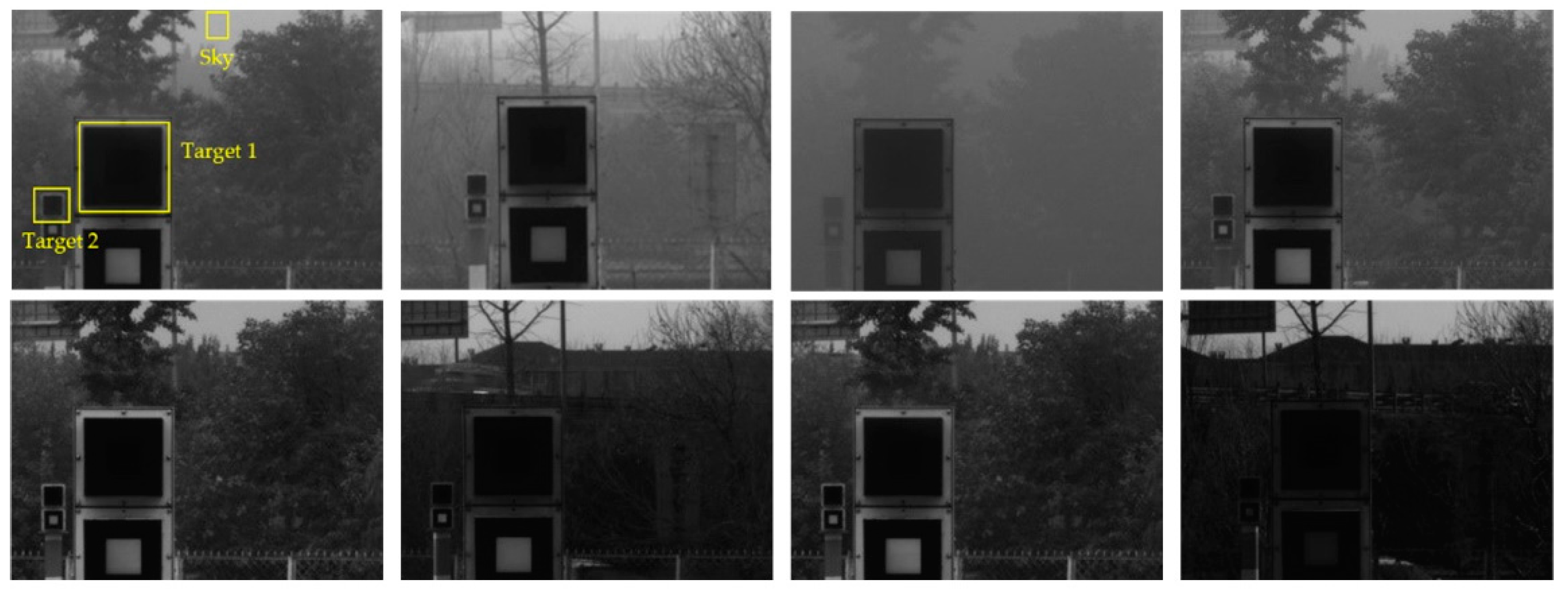
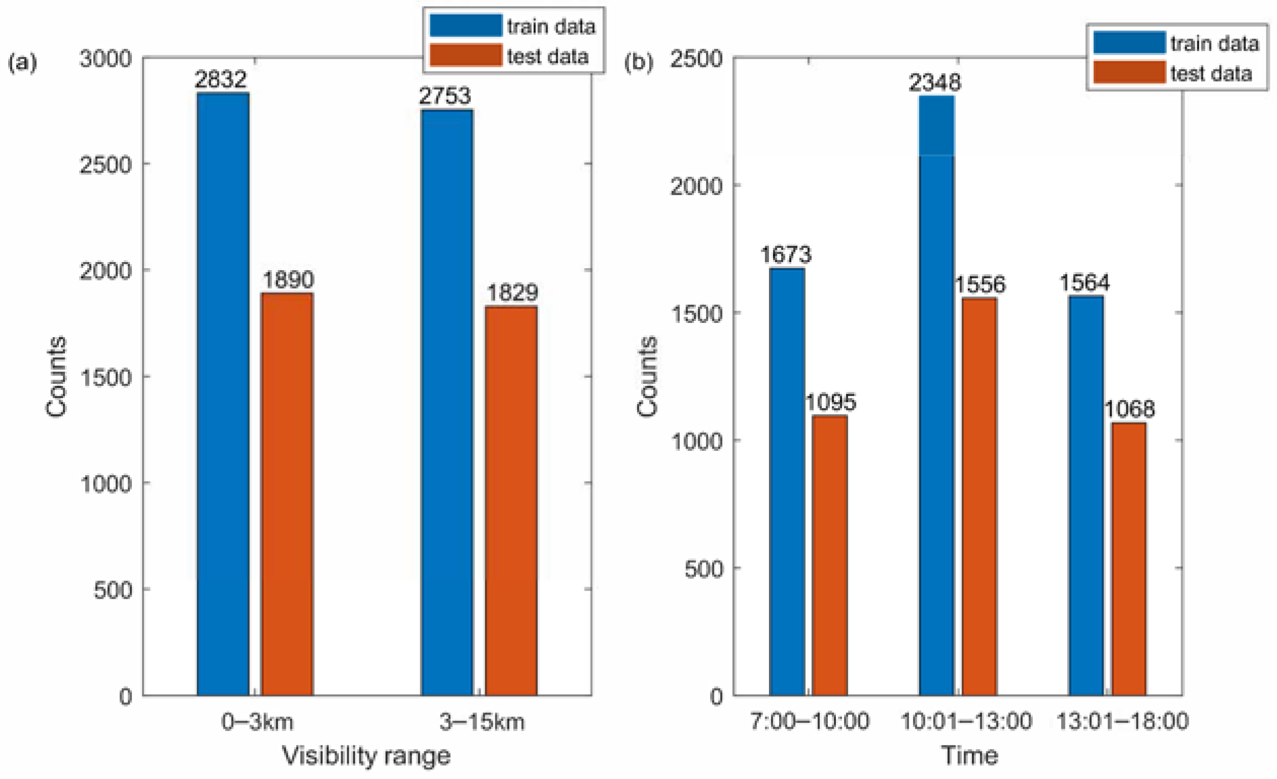
Typical images with 480 × 640 pixels from Visiometer 2 under different visibilities are shown in Figure 8. The grayscale images cannot show the strength of the radiance directly because of the different exposure times. The transmissometer LT31 recorded data every minute, and so did Visiometer 2. A total of 9304 images with a good quality (underexposed or overexposed images were eliminated) from Visiometer 2 were chosen for analysis. The numbers of images in the training and test datasets were 5585 and 3719, respectively. The images were randomly chosen and were not repetitive in the training dataset and test dataset. In every dataset, the numbers of samples for two classes (0–3 km and 3–15 km) were approximately equal, as shown in Figure 9a. Additionally, the images were approximately uniformly distributed over the day, as shown in Figure 9b. It should be noted that daytime data (7:30–17:59 local time) were utilized. The dataset contained images of as many situations as possible, such as an overcast sky, cloudy sky, clear sky, and so on.

Before training the images, preprocessing was required, including labeling and resizing the images. The labels were tagged after categorizing the images. The images’ labels were determined by the visibility value of the transmissometer LT31. If the visibility was greater than 3km, the image’s label was H. If the value was less than or equal to 3 km, the image’s label was L. Images with a lower resolution were processed faster. The images were reduced by using the bilinear interpolation method from 640 × 480 to 160 × 120. All the samples were processed without affecting the visibility features contained in the image.

4.2. Feature Extraction

The feature vector is an essential parameter in machine learning. The appropriate selection of feature vectors will make the process faster and the training results more accurate. The image feature that best represents atmospheric visibility is the edge information of the image. Since the atmosphere is equivalent to a low-pass filter, the edges of the objects in an image would be smoothed when under low visibility conditions. The Histograms of Oriented Gradients (HOG), which represent the edge information in an image, are used as the feature vectors in this paper.

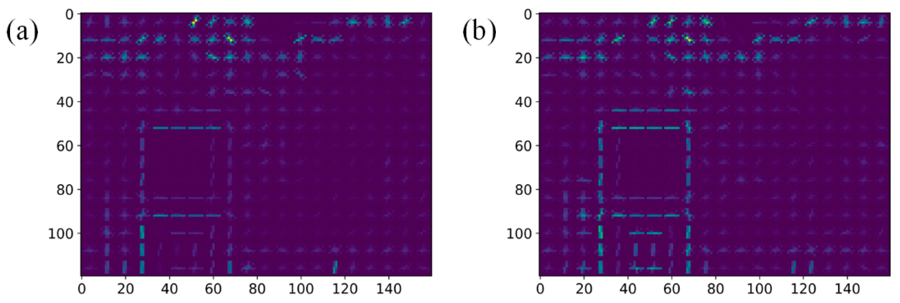
The resized image with 120 × 160 pixels was divided into 15 × 20 cells, each with 8 × 8 pixels, and the greyscale gradient of each pixel in the cell was calculated separately in the x and y directions. Therefore, each cell contained 128 values, including magnitudes and directions. The gradient vectors were grouped into nine bins with a 20-degree step from 0° to 180° according to the direction of the gradient. The corresponding amplitudes in each bin were added up. Thus, the three-dimensional arrays of 8 × 8 × 2 were reduced to a set of one-dimensional arrays containing nine numbers. Figure 10 shows the HOG features in different visibility conditions. A block defined by 3 × 3 cells was normalized by using L1 norms. By sliding a window with a step size of eight pixels, an image could generate 234 blocks. Eventually, an 18,954-dimensional array was obtained as a feature vector.

Some dimensions in the feature vector were not worthwhile for image discrimination. Therefore, it was necessary to reduce the dimensionality of the feature vector to speed up the operation. A Principal Component Analysis (PCA) was utilized to reduce the dimensions to 353, which contained a 90% contribution, as the feature vectors.

4.3. SVM Parameters

An SVM is a typical linear classification model based on the maximum interval of the feature space. Nonlinear classification can be achieved through kernel functions, which map the sample from n dimensions to n + 1 or higher dimensions.

Four kernel functions are commonly used in an SVM: a linear kernel, poly kernel, rbf (radial basis function or Gaussian kernel), and sigmoid Kernel. The dimensionality of a nonlinear kernel function (poly, rbf, and sigmoid) mapping is determined by the parameter gamma (the poly kernel also needs the degree to determine the highest power of the polynomial). Another key parameter of an SVM is the penalty factor C, which represents the tolerance for error. The penalty factor C has a significant effect on the prediction results of the model. The model will underfit if the C is too small, resulting in a low prediction accuracy. Conversely, a too-large C makes the model overfit and lose its generalizability.

The optimal parameters were selected by GridSearchCV from scikit-Learn (https://scikit-learn.org/stable/ (accessed on 22 May 2023). GridSearchCV iterates through all the candidate key parameters (

Table 1. The candidate parameters list.

Parameters	Candidate Value
C	(0.005, 0.01, 0.05, 0.1, 0.2, 0.3, 0.5, 1, 1.5, 2, 5, 10, 11, 13, 15, 20)
gamma	(0.001, 0.005, 0.01, 0.02, 0.03, 0.05, 0.1,0.3, 0.5, 0.7, 1, 2, 3, 4, 5, 8, 10)
degree	(0.5, 1, 2, 3, 4, 5)

), tests every possibility, and outputs the optimal performing parameters.

The optimal parameters and the performances of the four kernel functions are listed in

Table 2. Optimal parameters and fitting time of the model for different kernel functions.

Kernel Functions	C	Gamma	Degree	Fitting Time/s	10-Fold Mean Accuracy Score
RBF	5.0	0.03	--	0.22206	92.46%
poly	0.1	1.0	1.0	0.17827	92.48%
linear	0.3	--	--	0.1842	92.46%
sigmoid	13	0.02	--	0.22303	92.48%

. The performances of the optimal parameters were assessed by determining the 10-fold mean accuracy scores, and the accuracy score was defined as the ratio of all the correctly predicted samples to the total samples. A 10-fold cross validation was utilized because training with only one dataset tends to overfit the model, which indicates a good performance with this dataset but poor performance with other datasets. The mean accuracy scores of the four kernel functions were close and around 92.47%, while the “poly” and “linear” kernel functions had less fitting time. For simplicity’s sake, the model Bi-C with a “linear” kernel function and 0.3 of C was adopted.

4.4. Results

The images of the test dataset were processed by following step 1 and step 2 in Algorithm 1 and were classified by Bi-C. The confusion matrix of the test dataset is shown in

Table 3. Confusion matrix for the test dataset.

	Predict L	Predict H
True L	1865	25
True H	95	1734

. A total of 3599 images were classified correctly, and the accuracy score was 96.77%. Under the low visibility condition, 1865 images were correctly classified as L, but 25 images were classified as H; therefore, the error rate was 1.32%. Additionally, in 1829 images labeled H, 95 images were classified as L, and the error rate was 5.19%. This indicates that the classifier Bi-C had a better performance under low visibility conditions. This approach can provide a more accurate qualitative assessment of the atmospheric visibility status under complex conditions. The classification results can serve as dependable reference information for the visiometer with double targets.

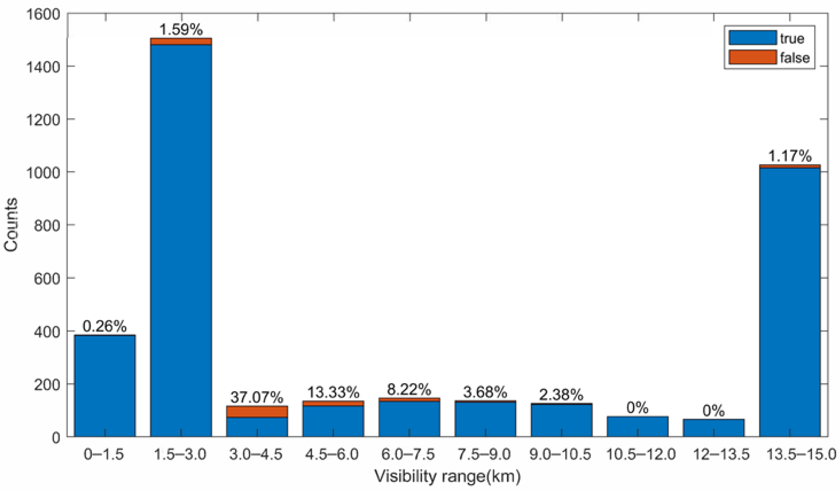
The distribution of the false predicted images with respect to visibility is shown in Figure 11. The performance was worse in the range of 4 km–10.5 km probably due to the fewer number of samples, especially in 3.0 km–4.5 km with a false rate of 37.07%. Another reason for the high false rate in 3.0 km–4.5 km was that the model had a flaw at the visibility near 3 km. Visibility is a continuous absolute value, so the classification would have a very low tolerance around the classification line. In future studies, a new classification standard should be proposed to evaluate the results of the near visibility limit value.

5. Conclusions

For a camera-based visiometer, even with artificial blackbodies, visibility measurements calculated by using contrast may still be highly inaccurate under high-visibility conditions [5,6,26,27]. We suggest that the errors that occur at high visibility may be caused by nonstandard observation conditions. Several nonstandard observation conditions have been described by Horvath [25] and Allard [28]; however, a comprehensive analysis of the visibility measurement errors with the artificial blackbody targets was not carried out. By using visiometers with double blackbody targets, this study summarizes the nonstandard conditions into two categories: errors introduced by the sky background not being right behind the target, which causes that the scattered light from the atmosphere, $B_{IN}$, to be unable to be cancelled out, and the errors introduced by inhomogeneous illumination conditions causing inconsistencies between the inherent sky brightness behind the two targets.

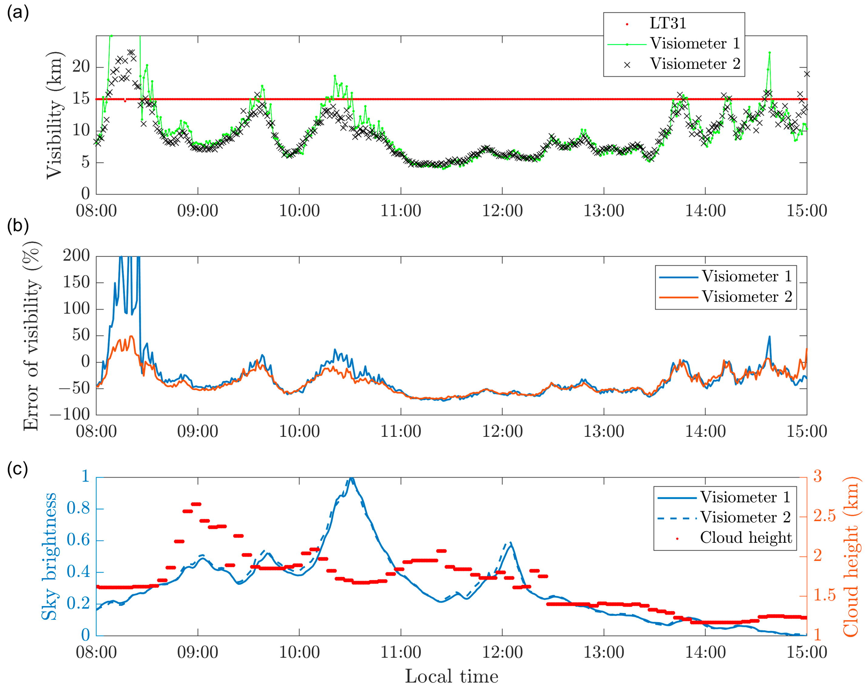
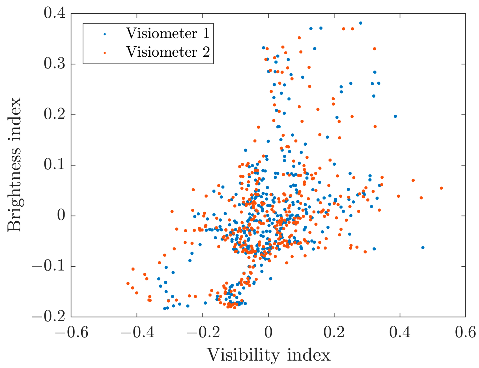
To demonstrate the effects of the observing environment on the visibility measurements, two separate and identical visiometers with two blackbody targets were used in this study. Both visiometers used the same blackbody structures, cameras, and calibration methods to avoid systematic errors. They were installed in the same area to ensure that both visiometers were subject to the same environmental influences. The observations of two visiometers demonstrated that the visibility measurements tended to have large errors when under high visibility and nonstandard conditions, and the visibility results were related to sky background brightness, which conflicts with Koschmieder’s theory. In Koschmieder’s theory, visibility is only determined by the atmospheric extinction coefficient, and the effect of the sky brightness is eliminated by the contrast with the target brightness. So, the relevance between the visibility values and the sky brightness confirms that the effect of inhomogeneous conditions is nonnegligible when using the contrast-based method. Additionally, we found that the inhomogeneous sky brightness may be caused by clouds because the sky background brightness variation was consistent with the variation in the cloud height. The effect of the clouds should be investigated in detail in future studies, and utilizing comprehensive cloud information to calibrate the visibility measurements may be a potential method.

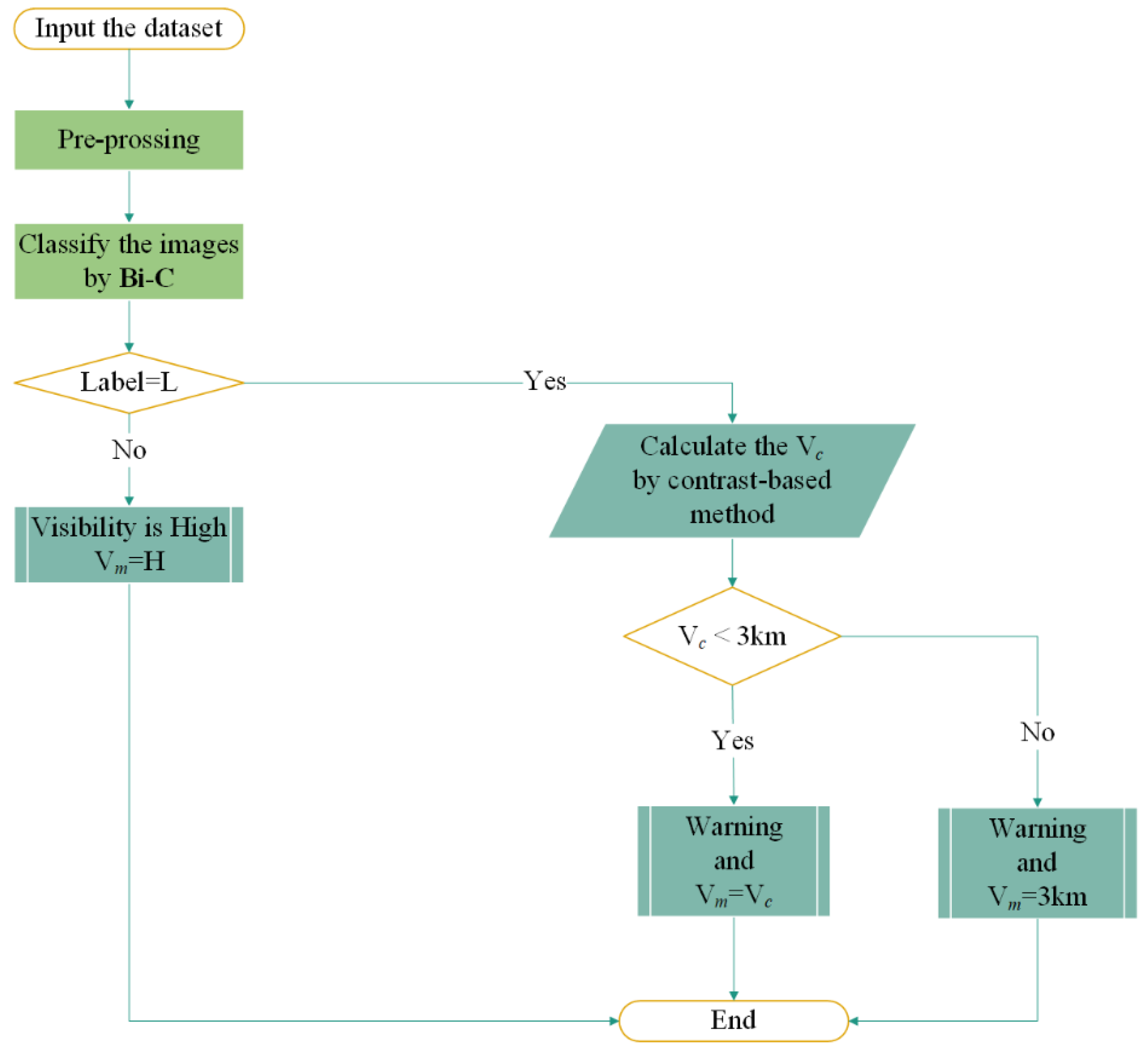
So, a reliable method is required to complement the contrast-based method under all conditions. We proposed an SVM-based binary classification model for the qualitative classification of images with an accuracy of 96.77%. This model does not provide accurate absolute visibility values, but, to a great extent, it guarantees the accuracy of image recognition compared to other multiclassification models. Furthermore, in combination with the contrast-based method, accurate absolute visibility values can be obtained under low visibility conditions. As shown in Figure 12, following preprocessing of the image data with resizing and feature extraction, the Bi-C model is used for classification. An image identified as H means the visibility is above 3 km, which is not a threat to traffic safety; an image identified as L means the visibility is below 3 km and a warning is required; additionally, the absolute visibility value $V_c$ is calculated by using the contrast-based method. If $V_c$ is below 3 km, this value is considered the true visibility measurement $V_m$; if $V_c$ is above 3 km, 3 km is considered the true visibility measurement $V_m$. This warning system provides an accurate and reliable information reference for decision makers in the transport department and helps them ensure a safe and smooth flow of traffic.

The model Bi-C initially achieved a reliable classification under low visibility conditions, but it has some limitations:

(1)

The Bi-C model was trained on the image dataset shown in Figure 8, so the model ensures an accurate classification of the image from the Visiometer 2 in Figure 5 and is not applicable to other scenes or systems.

(2)

Images were inspected with a quality control algorithm before classification, and overexposed or underexposed images were excluded because underexposure or overexposure affects the edge information of the image, which is an important parameter in determining visibility. These types of images were not only not applicable to the SVM-based method, but they were also not applicable to the contrast-based method. Therefore, images that are underexposed or overexposed are an unavoidable issue for visiometers. An effective exposure range helps to automatically screen images, reduce visibility estimation errors, and enable fully automated visibility observations.

(3)

The identification of low visibility was the primary concern of this study, while there is still a demand for accurate visibility measurements. In future research, multiple classification identification and regression prediction methods for visibility should be explored to improve the precision of the visibility measurements.