
A Coupled CH4, CO and CO2 Simulation for Improved Chemical Source Modeling


Abstract
:1. Introduction
2. Methods
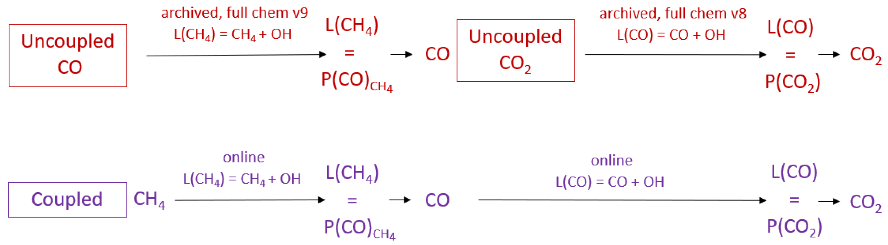
2.1. Uncoupled GEOS-Chem Carbon Gas Simulations

| CH | CO | CO | |
|---|---|---|---|
| Fields used by both uncoupled and coupled simulations | |||
| Stratospheric L(CH) | Archived fields 1 | - | - |
| Stratospheric L(CO) | - | GMI 2 | - |
| Stratospheric P(CO) | - | GMI 2 | - |
| P(CO) | - | P(CO) = P(CO) − P(CO) | - |
| - | archived, full chemistry v9-01-03 3 | - | |
| Fields used by uncoupled simulations only | |||
| L(CH) 4 | online 5 | archived, full chemistry v9-01-03 3 | - |
| Time resolution | Every model timestep, 20 min | Monthly mean, 2009–2011 average | - |
| - | archived, = Trop. L(CH) | - | |
| Time resolution | - | Monthly mean, 2009–2011 average | - |
| L(CO) 4,6 | - | online, v9-01-03 [OH] 3 | archived, full chemistry v8-02-01 7 |
| Time resolution | - | Every model timestep, 20 min | Monthly mean, 2004–2010 |
| P(CO) 6 | - | - | archived, P(CO) = L(CO) |
| Time resolution | - | - | Monthly mean, 2004–2010 |
| Fields used by coupled simulation only | |||
| L(CH) | online, v9-01-03 [OH] 3,8 | - | - |
| Time resolution | Every model timestep, 20 min | - | - |
| - | online, P(CO) = L(CH) | - | |
| Time resolution | - | Every model timestep, 20 min | - |
| L(CO) | - | online, v9-01-03 [OH] 3 | - |
| Time resolution | - | Every model timestep, 20 min | - |
| P(CO) 9 | - | - | online, P(CO) = L(CO) |
| Time resolution | - | Every model timestep, 20 min | |
2.2. Coupled GEOS-Chem Simulation
2.3. Experimental Design
3. Results and Discussions
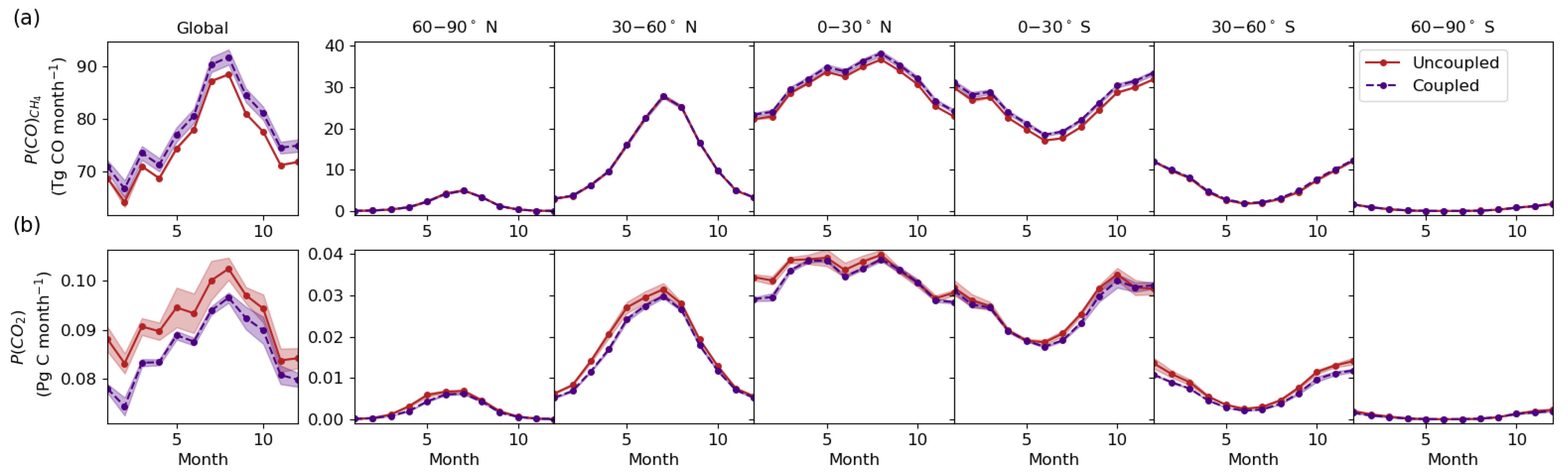
3.1. Chemical Production Budgets
3.2. Chemical Source Contributions
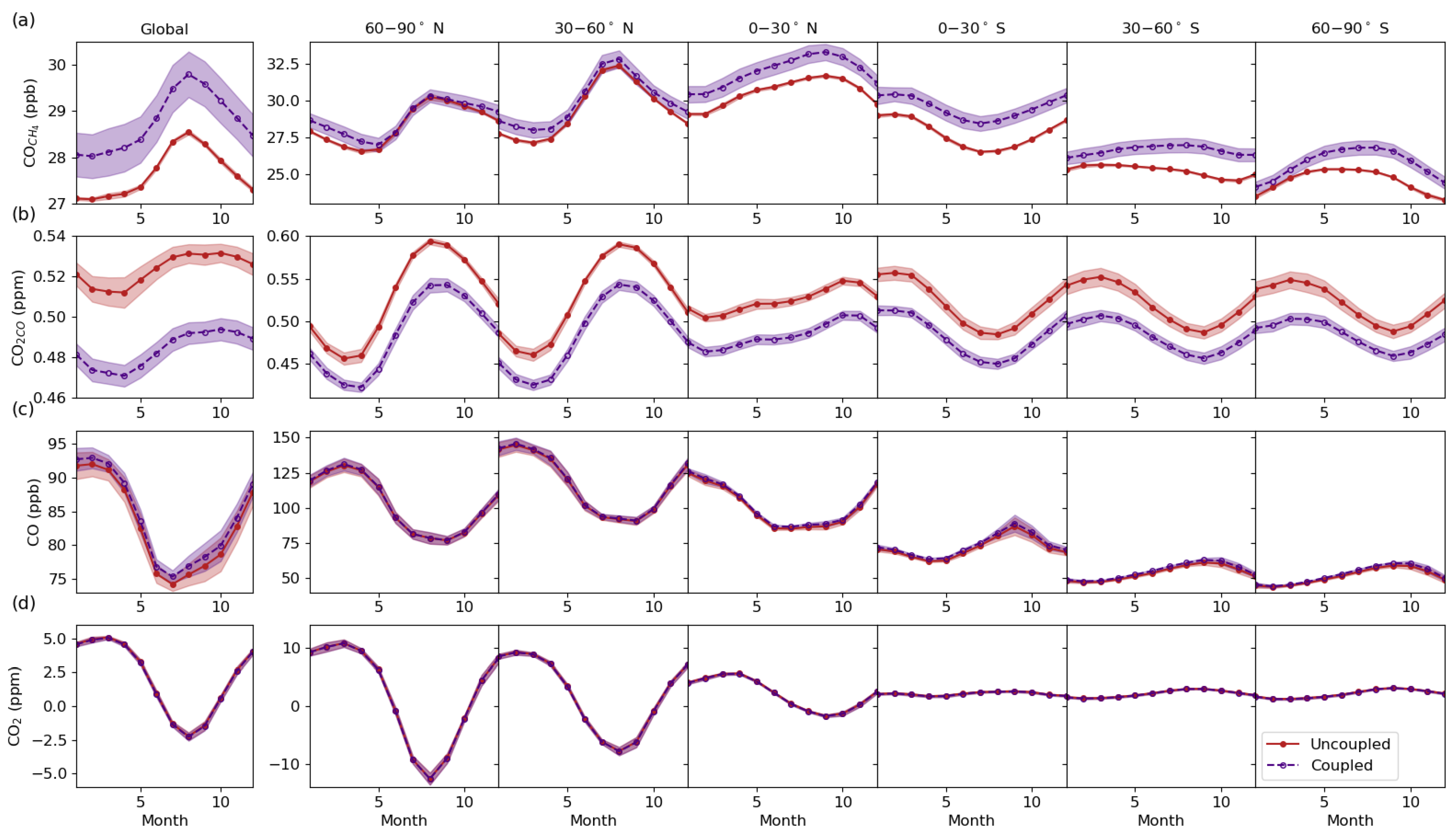
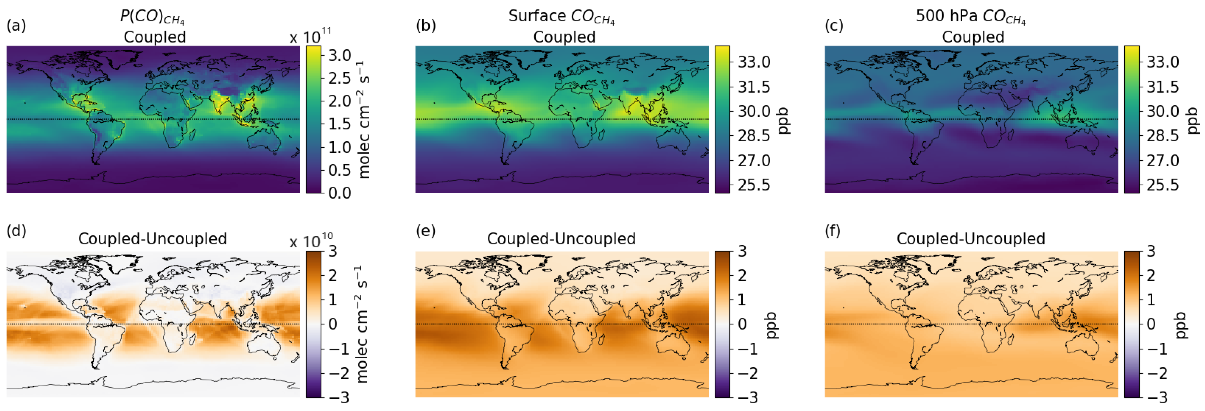
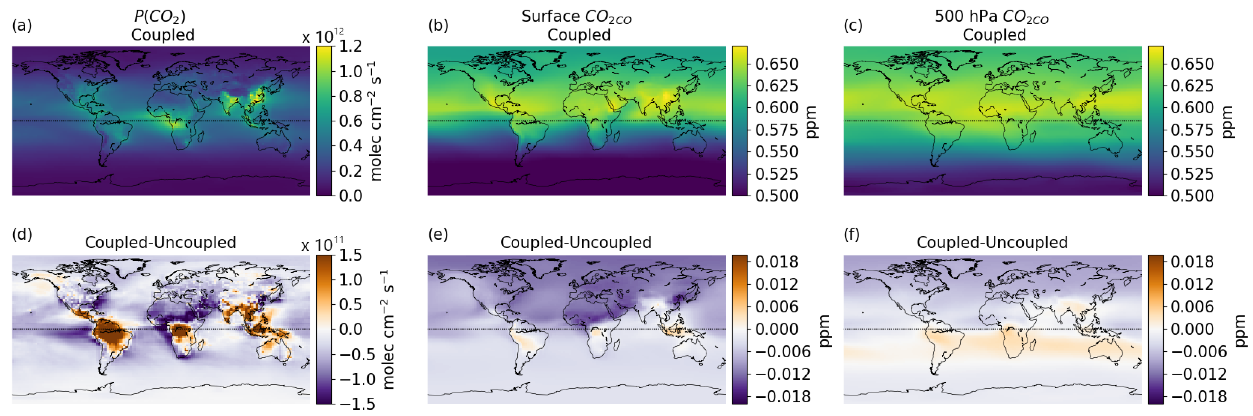
3.3. Global Distribution
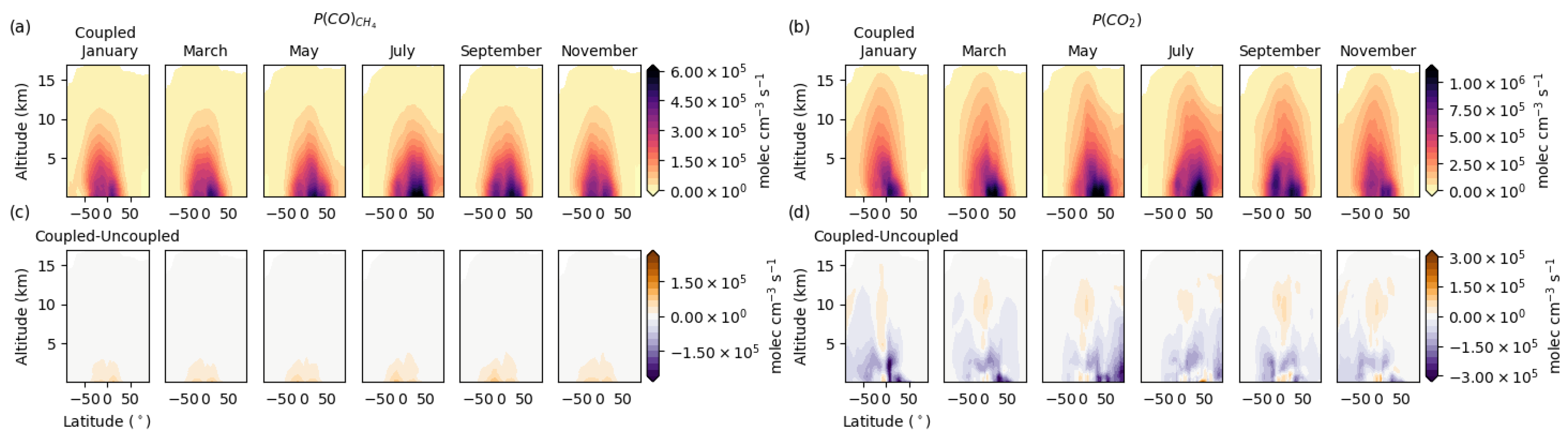
3.4. Vertical Latitudinal Distribution
3.5. Model Evaluation with Column, Surface and Aircraft Measurements
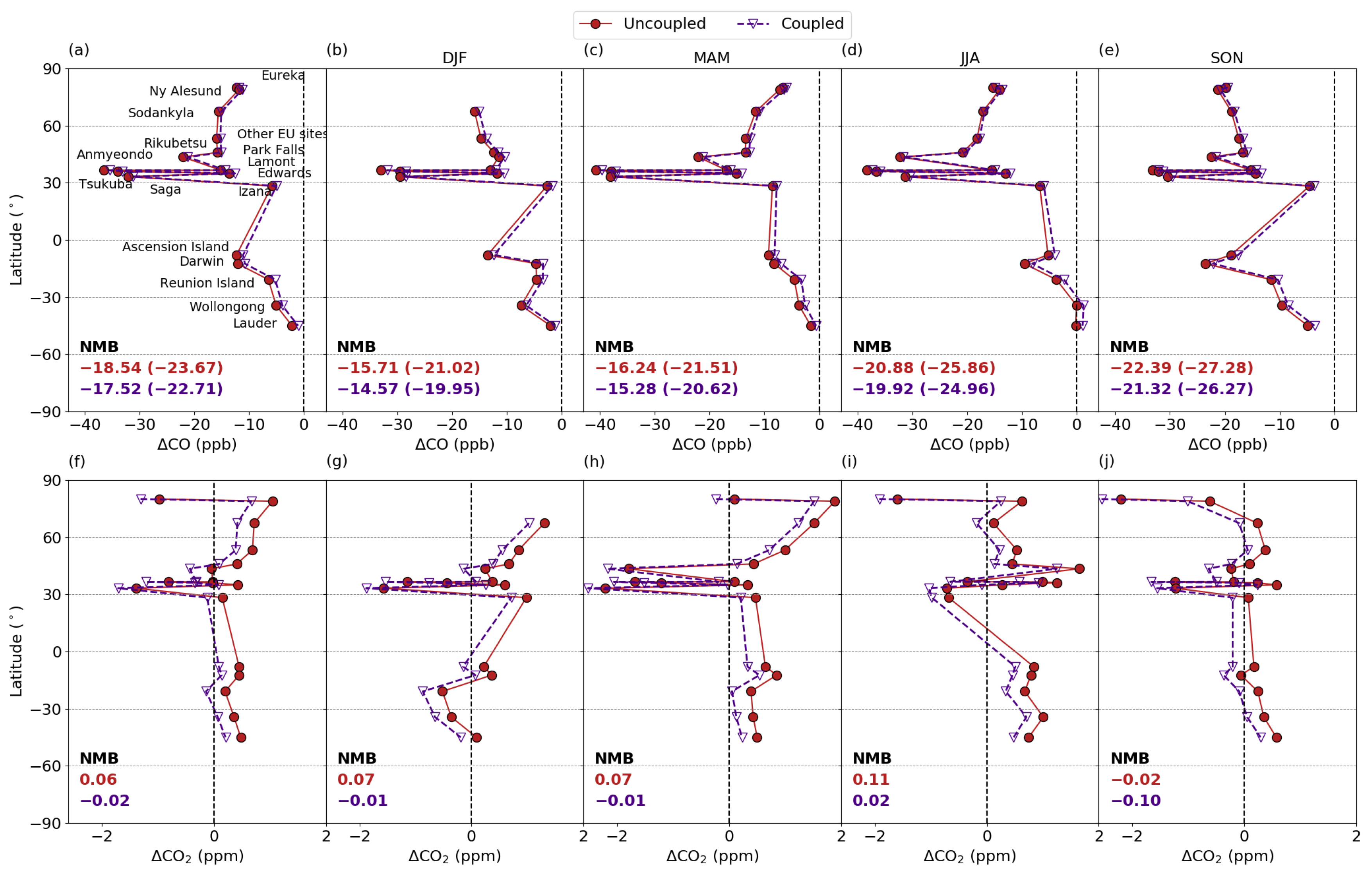
3.5.1. Comparison with column measurements
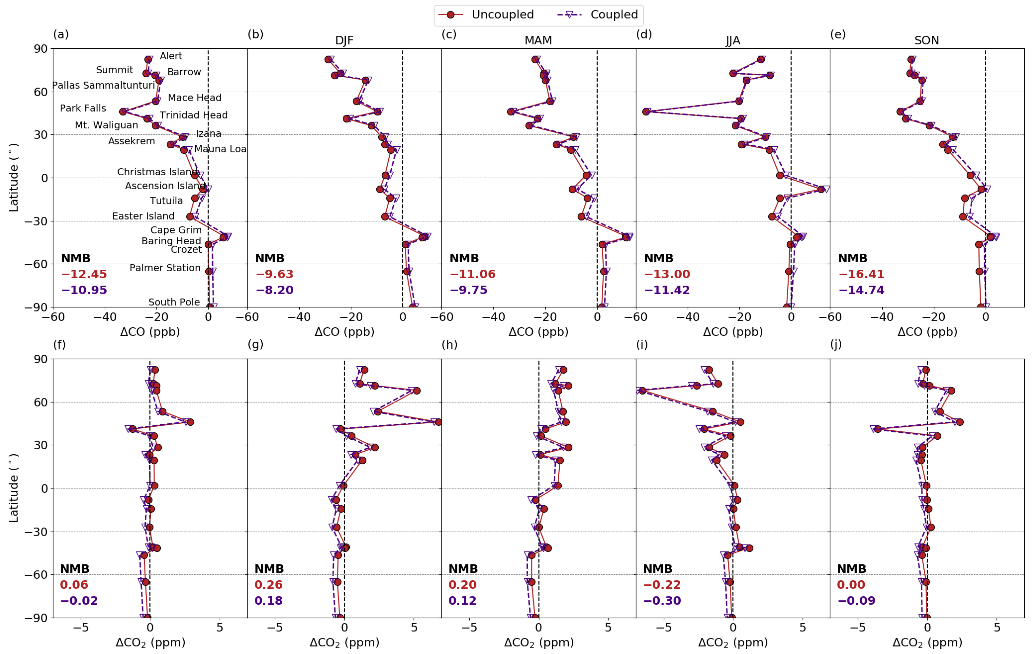
3.5.2. Comparison with Surface Measurements
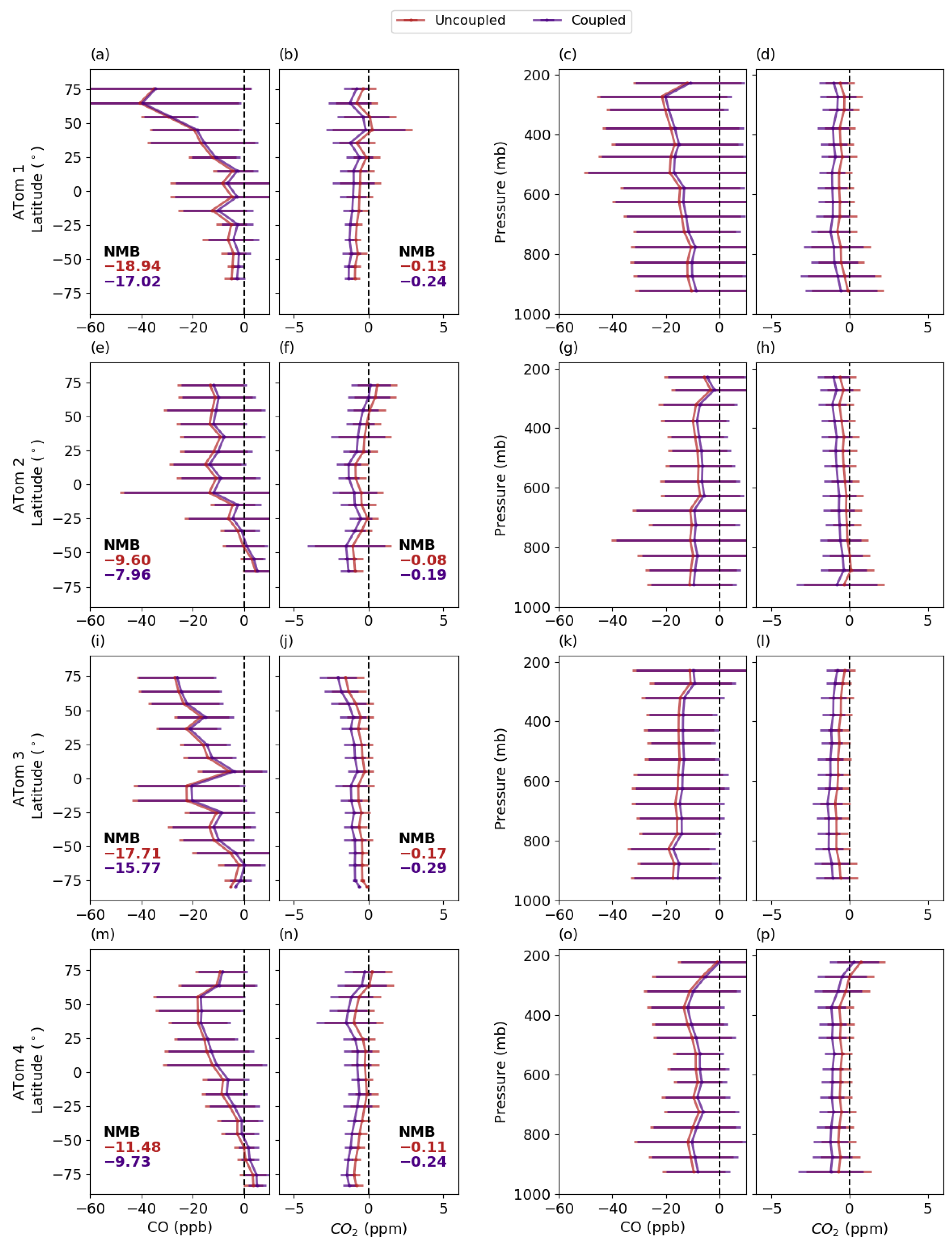
3.5.3. Comparison with Aircraft Measurements
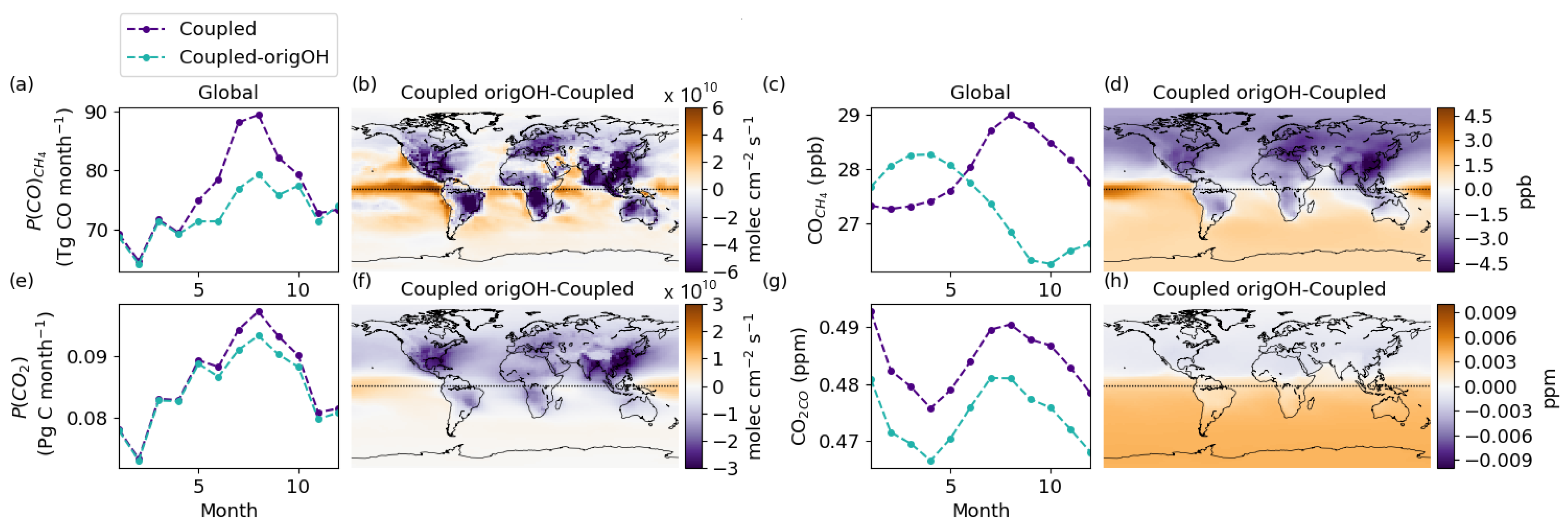
3.6. The Importance of Consistent OH Fields
4. Conclusions
Supplementary Materials
Author Contributions
Funding
Institutional Review Board Statement
Informed Consent Statement
Data Availability Statement
Acknowledgments
Conflicts of Interest
Appendix A
| Station | Latitude | Longitude | Elevation (m) |
|---|---|---|---|
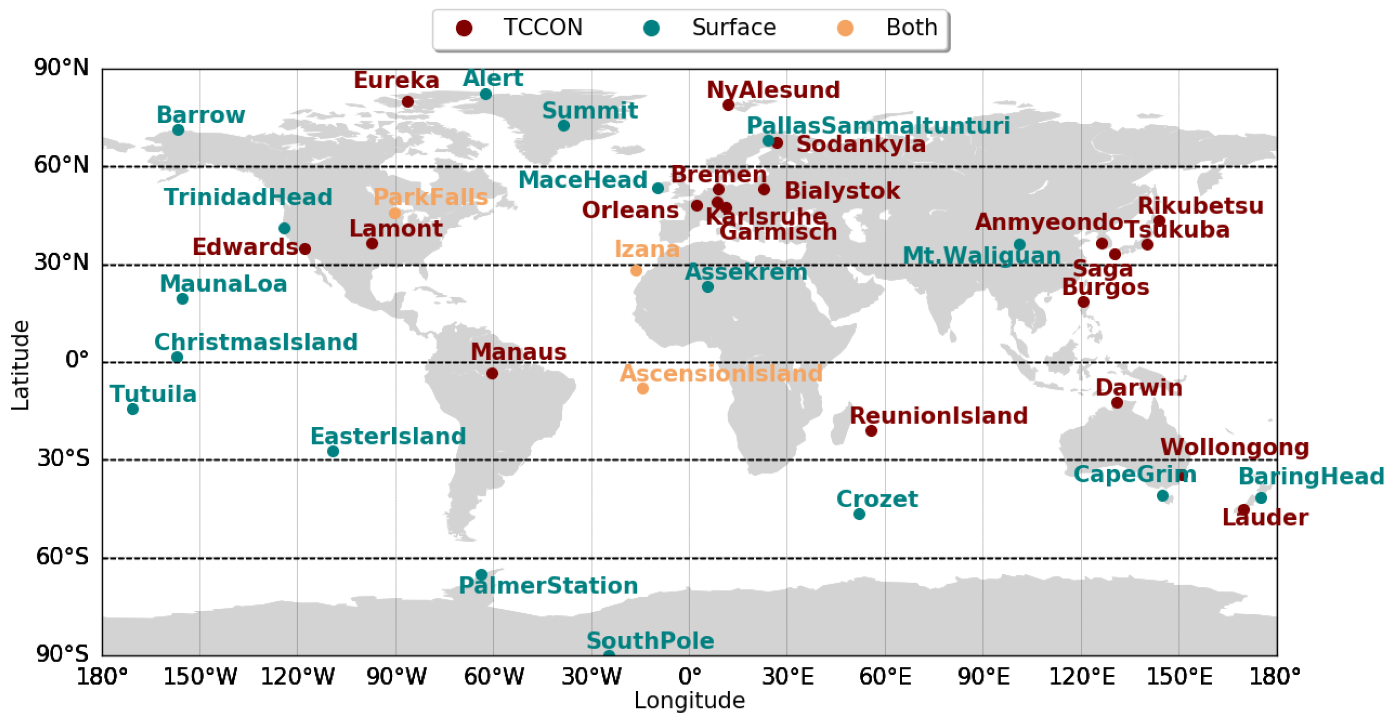
| TCCON sites | |||
| Eureka 1 | 80.05 N | 86.42 W | 610 |
| Ny Alesund 2 | 78.90 N | 11.89 E | 20 |
| Sodankyla 3 | 67.37 N | 26.63 E | 188 |
| Białystok 4 | 53.23 N | 23.02 E | 180 |
| Bremen 5 | 53.10 N | 8.85 E | 27 |
| Karlsruhe 6 | 49.10 N | 8.43 E | 116 |
| Orléans 7 | 47.97 N | 2.11 E | 130 |
| Garmisch 8 | 47.48 N | 11.06 E | 740 |
| Rikubetsu 9 | 43.46 N | 143.77 E | 380 |
| Lamont 10 | 36.60 N | 97.49 W | 320 |
| Anmyeondo 11 | 36.54 N | 126.33 E | 30 |
| Tsukuba 12 | 36.05 N | 140.12 E | 30 |
| Edwards 13 | 34.96 N | 117.88 W | 699 |
| Saga 14 | 33.24 N | 130.29 E | 7 |
| Burgos 15 | 18.53 N | 120.62 E | 35 |
| Manaus 16 | 3.21 S | 60.60 W | 50 |
| Darwin 17 | 12.43 S | 130.89 E | 30 |
| Reunion Island 18 | 20.90 S | 55.48 E | 87 |
| Wollongong 19 | 34.41 S | 150.88 E | 30 |
| Lauder 20 | 45.04 S | 169.68 E | 370 |
| Both TCCON sites and surface 24,25,26 | |||
| Park Falls 21 | 45.94 N | 90.27 W | 440 |
| Izana 22 | 28.30 N | 16.50 W | 2370 |
| Ascension Island 23 | 7.91 S | 14.33 W | 10 |
| Surface sites 24,25,26 | |||
| Alert | 82.45 N | 62.51 W | 185 |
| Summit | 72.50 N | 38.42 W | 3209 |
| Barrow | 71.32 N | 156.61 W | 11 |
| Pallas Sammaltunturi | 67.97 N | 24.12 E | 565 |
| Mace Head | 53.33 N | 9.89 W | 5 |
| Trinidad Head | 41.06 N | 124.15 W | 107 |
| Mt. Waliguan | 36.29 N | 100.89 E | 3810 |
| Assekrem | 23.26 N | 5.63 E | 2710 |
| Mauna Loa | 19.53 N | 155.58 W | 3397 |
| Christmas Island | 1.70 N | 157.15 W | 0 |
| Tutuila | 14.25 S | 170.56 W | 42 |
| Easter Island | 27.16 S | 109.43 W | 47 |
| Cape Grim | 40.67 S | 144.69 E | 94 |
| Baring Head | 41.41 S | 174.87 E | 85 |
| Crozet | 46.43 S | 51.84 E | 197 |
| Palmer Station | 64.77 S | 64.05 W | 10 |
| South Pole | 89.98 S | 24.80 W | 2810 |
References
- Stocker, T.; Qin, D.; Plattner, G.K.; Tignor, M.; Allen, S.; Boschung, J.; Nauels, A.; Xia, Y.; Bex, V.; Midgley, P. IPCC, 2013: Climate Change 2013: The Physical Science Basis. Contribution of Working Group I to the Fifth Assessment Report of the Intergovernmental Panel on Climate Change; Cambridge University Press: Cambridge, UK, 2014. [Google Scholar]
- Shindell, D.T.; Faluvegi, G.; Bell, N.; Schmidt, G.A. An emissions-based view of climate forcing by methane and tropospheric ozone. Geophys. Res. Lett. 2005, 32. [Google Scholar] [CrossRef]
- Bousquet, P.; Ciais, P.; Miller, J.; Dlugokencky, E.; Hauglustaine, D.; Prigent, C.; Van der Werf, G.; Peylin, P.; Brunke, E.G.; Carouge, R.; et al. Contribution of anthropogenic and natural sources to atmospheric methane variability. Nature 2006, 443, 439–443. [Google Scholar] [CrossRef]
- Duncan, B.N.; Logan, J.A.; Bey, I.; Megretskaia, I.A.; Yantosca, R.M.; Novelli, P.C.; Jones, N.B.; Rinsland, C.P. Global budget of CO, 1988–1997: Source estimates and validation with a global model. J. Geophys. Res. Atmos. 2007, 112. [Google Scholar] [CrossRef]
- Liu, J.; Bowman, K.W.; Schimel, D.S.; Parazoo, N.C.; Jiang, Z.; Lee, M.; Bloom, A.A.; Wunch, D.; Frankenberg, C.; Sun, Y.; et al. Contrasting carbon cycle responses of the tropical continents to the 2015–2016 El Niño. Science 2017, 358, eaam5690. [Google Scholar] [CrossRef]
- Bloom, A.A.; Bowman, K.W.; Lee, M.; Turner, A.J.; Schroeder, R.; Worden, J.R.; Weidner, R.; McDonald, K.C.; Jacob, D.J. A global wetland methane emissions and uncertainty dataset for atmospheric chemical transport models (WetCHARTs version 1.0). Geosci. Model Dev. 2017, 10, 2141–2156. [Google Scholar] [CrossRef]
- Turner, A.J.; Jacob, D.J.; Wecht, K.J.; Maasakkers, J.D.; Lundgren, E.; Andrews, A.E.; Biraud, S.C.; Boesch, H.; Bowman, K.W.; Deutscher, N.M.; et al. Estimating global and North American methane emissions with high spatial resolution using GOSAT satellite data. Atmos. Chem. Phys. 2015, 15, 7049–7069. [Google Scholar] [CrossRef]
- Wang, J.S.; Logan, J.A.; McElroy, M.B.; Duncan, B.N.; Megretskaia, I.A.; Yantosca, R.M. A 3-D model analysis of the slowdown and interannual variability in the methane growth rate from 1988 to 1997. Glob. Biogeochem. Cycles 2004, 18. [Google Scholar] [CrossRef]
- Messerschmidt, J.; Parazoo, N.; Wunch, D.; Deutscher, N.M.; Roehl, C.; Warneke, T.; Wennberg, P.O. Evaluation of seasonal atmosphere–biosphere exchange estimations with TCCON measurements. Atmos. Chem. Phys. 2013, 13, 5103–5115. [Google Scholar] [CrossRef]
- Bukosa, B.; Deutscher, N.M.; Fisher, J.A.; Kubistin, D.; Paton-Walsh, C.; Griffith, D.W.T. Simultaneous shipborne measurements of CO2, CH4 and CO and their application to improving greenhouse-gas flux estimates in Australia. Atmos. Chem. Phys. 2019, 19, 7055–7072. [Google Scholar] [CrossRef]
- Kopacz, M.; Jacob, D.J.; Fisher, J.A.; Logan, J.A.; Zhang, L.; Megretskaia, I.A.; Yantosca, R.M.; Singh, K.; Henze, D.K.; Burrows, J.P.; et al. Global estimates of CO sources with high resolution by adjoint inversion of multiple satellite datasets (MOPITT, AIRS, SCIAMACHY, TES). Atmos. Chem. Phys. 2010, 10, 855–876. [Google Scholar] [CrossRef]
- Palmer, P.I.; Jacob, D.J.; Jones, D.B.A.; Heald, C.L.; Yantosca, R.M.; Logan, J.A.; Sachse, G.W.; Streets, D.G. Inverting for emissions of carbon monoxide from Asia using aircraft observations over the western Pacific. J. Geophys. Res. Atmos. 2003, 108, 8828. [Google Scholar] [CrossRef]
- Enting, I.G.; Mansbridge, J.V. Latitudinal distribution of sources and sinks of CO2: Results of an inversion study. Tellus B 1991, 43, 156–170. [Google Scholar] [CrossRef]
- Suntharalingam, P.; Randerson, J.T.; Krakauer, N.; Logan, J.A.; Jacob, D.J. Influence of reduced carbon emissions and oxidation on the distribution of atmospheric CO2: Implications for inversion analyses. Glob. Biogeochem. Cycles 2005, 19, GB4003. [Google Scholar] [CrossRef]
- Nassar, R.; Jones, D.B.A.; Suntharalingam, P.; Chen, J.M.; Andres, R.J.; Wecht, K.J.; Yantosca, R.M.; Kulawik, S.S.; Bowman, K.W.; Worden, J.R.; et al. Modeling global atmospheric CO2 with improved emission inventories and CO2 production from the oxidation of other carbon species. Geosci. Model Dev. 2010, 3, 689–716. [Google Scholar] [CrossRef]
- Wecht, K.J.; Jacob, D.J.; Frankenberg, C.; Jiang, Z.; Blake, D.R. Mapping of North American methane emissions with high spatial resolution by inversion of SCIAMACHY satellite data. J. Geophys. Res. Atmos. 2014, 119, 7741–7756. [Google Scholar] [CrossRef]
- Fisher, J.A.; Murray, L.T.; Jones, D.B.A.; Deutscher, N.M. Improved method for linear carbon monoxide simulation and source attribution in atmospheric chemistry models illustrated using GEOS-Chem v9. Geosci. Model Dev. Discuss. 2017, 2017, 4129–4144. [Google Scholar] [CrossRef]
- Jacob, D.J. Introduction to Atmospheric Chemistry; Princeton University Press: Princeton, NJ, USA, 1999. [Google Scholar]
- Isaksen, I.S.; Hov, Ø. Calculation of trends in the tropospheric concentration of O3, OH, CO, CH4 and NOx. Tellus B 1987, 39B, 271–285. [Google Scholar] [CrossRef]
- Folberth, G.; Hauglustaine, D.A.; Ciais, P.; Lathière, J. On the role of atmospheric chemistry in the global CO2 budget. Geophys. Res. Lett. 2005, 32, L08801. [Google Scholar] [CrossRef]
- Logan, J.A.; Prather, M.J.; Wofsy, S.C.; McElroy, M.B. Tropospheric chemistry: A global perspective. J. Geophys. Res. Ocean. 1981, 86, 7210–7254. [Google Scholar] [CrossRef]
- Tie, X.; Jim Kao, C.Y.; Mroz, E. Net yield of OH, CO, and O3 from the oxidation of atmospheric methane. Atmos. Environ. Part A Gen. Top. 1992, 26, 125–136. [Google Scholar] [CrossRef]
- Manning, M.R.; Brenninkmeijer, C.A.M.; Allan, W. Atmospheric carbon monoxide budget of the southern hemisphere: Implications of 13C/12C measurements. J. Geophys. Res. Atmos. 1997, 102, 10673–10682. [Google Scholar] [CrossRef]
- Novelli, P.C.; Lang, P.M.; Masarie, K.A.; Hurst, D.F.; Myers, R.; Elkins, J.W. Molecular hydrogen in the troposphere: Global distribution and budget. J. Geophys. Res. Atmos. 1999, 104, 30427–30444. [Google Scholar] [CrossRef]
- Bergamaschi, P.; Hein, R.; Brenninkmeijer, C.A.M.; Crutzen, P.J. Inverse modeling of the global CO cycle: 2. Inversion of 13C/12C and 18O/16O isotope ratios. J. Geophys. Res. Atmos. 2000, 105, 1929–1945. [Google Scholar] [CrossRef]
- Franco, B.; Blumenstock, T.; Cho, C.; Clarisse, L.; Clerbaux, C.; Coheur, P.F.; De Mazière, M.; De Smedt, I.; Dorn, H.P.; Emmerichs, T.; et al. Ubiquitous atmospheric production of organic acids mediated by cloud droplets. Nature 2021, 593, 233–237. [Google Scholar] [CrossRef] [PubMed]
- Holloway, T.; Levy II, H.; Kasibhatla, P. Global distribution of carbon monoxide. J. Geophys. Res. Atmos. 2000, 105, 12123–12147. [Google Scholar] [CrossRef]
- Arellano, A.F., Jr.; Hess, P.G. Sensitivity of top-down estimates of CO sources to GCTM transport. Geophys. Res. Lett. 2006, 33, L21807. [Google Scholar] [CrossRef]
- Stein, O.; Schultz, M.G.; Bouarar, I.; Clark, H.; Huijnen, V.; Gaudel, A.; George, M.; Clerbaux, C. On the wintertime low bias of Northern Hemisphere carbon monoxide found in global model simulations. Atmos. Chem. Phys. 2014, 14, 9295–9316. [Google Scholar] [CrossRef]
- Zeng, G.; Williams, J.E.; Fisher, J.A.; Emmons, L.K.; Jones, N.B.; Morgenstern, O.; Robinson, J.; Smale, D.; Paton-Walsh, C.; Griffith, D.W.T. Multi-model simulation of CO and HCHO in the Southern Hemisphere: Comparison with observations and impact of biogenic emissions. Atmos. Chem. Phys. 2015, 15, 7217–7245. [Google Scholar] [CrossRef]
- Pétron, G.; Granier, C.; Khattatov, B.; Yudin, V.; Lamarque, J.F.; Emmons, L.; Gille, J.; Edwards, D.P. Monthly CO surface sources inventory based on the 2000–2001 MOPITT satellite data. Geophys. Res. Lett. 2004, 31, L21107. [Google Scholar] [CrossRef]
- Le Quéré, C.; Andrew, R.M.; Friedlingstein, P.; Sitch, S.; Hauck, J.; Pongratz, J.; Pickers, P.A.; Korsbakken, J.I.; Peters, G.P.; Canadell, J.G.; et al. Global Carbon Budget 2018. Earth Syst. Sci. Data 2018, 10, 2141–2194. [Google Scholar] [CrossRef]
- Ciais, P.; Borges, A.V.; Abril, G.; Meybeck, M.; Folberth, G.; Hauglustaine, D.; Janssens, I.A. The impact of lateral carbon fluxes on the European carbon balance. Biogeosciences 2008, 5, 1259–1271. [Google Scholar] [CrossRef]
- Elshorbany, Y.F.; Duncan, B.N.; Strode, S.A.; Wang, J.S.; Kouatchou, J. The description and validation of the computationally Efficient CH4–CO–OH (ECCOHv1.01) chemistry module for 3-D model applications. Geosci. Model Dev. 2016, 9, 799–822. [Google Scholar] [CrossRef]
- Pison, I.; Bousquet, P.; Chevallier, F.; Szopa, S.; Hauglustaine, D. Multi-species inversion of CH4, CO and H2 emissions from surface measurements. Atmos. Chem. Phys. 2009, 9, 5281–5297. [Google Scholar] [CrossRef]
- Wang, H.; Jacob, D.J.; Kopacz, M.; Jones, D.B.A.; Suntharalingam, P.; Fisher, J.A.; Nassar, R.; Pawson, S.; Nielsen, J.E. Error correlation between CO2 and CO as constraint for CO2 flux inversions using satellite data. Atmos. Chem. Phys. 2009, 9, 7313–7323. [Google Scholar] [CrossRef]
- Pandey, S.; Houweling, S.; Krol, M.; Aben, I.; Röckmann, T. On the use of satellite-derived CH4: CO2 columns in a joint inversion of CH4 and CO2 fluxes. Atmos. Chem. Phys. 2015, 15, 8615–8629. [Google Scholar] [CrossRef]
- Nassar, R.; Napier-Linton, L.; Gurney, K.R.; Andres, R.J.; Oda, T.; Vogel, F.R.; Deng, F. Improving the temporal and spatial distribution of CO2 emissions from global fossil fuel emission data sets. J. Geophys. Res. Atmos. 2013, 118, 917–933. [Google Scholar] [CrossRef]
- Maasakkers, J.D.; Jacob, D.J.; Sulprizio, M.P.; Scarpelli, T.R.; Nesser, H.; Sheng, J.X.; Zhang, Y.; Hersher, M.; Bloom, A.A.; Bowman, K.W.; et al. Global distribution of methane emissions, emission trends, and OH concentrations and trends inferred from an inversion of GOSAT satellite data for 2010–2015. Atmos. Chem. Phys. 2019, 19, 7859–7881. [Google Scholar] [CrossRef]
- Considine, D.B.; Logan, J.A.; Olsen, M.A. Evaluation of near-tropopause ozone distributions in the Global Modeling Initiative combined stratosphere/troposphere model with ozonesonde data. Atmos. Chem. Phys. 2008, 8, 2365–2385. [Google Scholar] [CrossRef]
- Allen, D.; Pickering, K.; Duncan, B.; Damon, M. Impact of lightning NO emissions on North American photochemistry as determined using the Global Modeling Initiative (GMI) model. J. Geophys. Res. Atmos. 2010, 115, D22301. [Google Scholar] [CrossRef]
- Murray, L.T.; Jacob, D.J.; Logan, J.A.; Hudman, R.C.; Koshak, W.J. Optimized regional and interannual variability of lightning in a global chemical transport model constrained by LIS/OTD satellite data. J. Geophys. Res. Atmos. 2012, 117, D20307. [Google Scholar] [CrossRef]
- Burkholder, J.B.; Sander, S.P.; Abbatt, J.; Barker, J.R.; Huie, R.E.; Kolb, C.E.; Kurylo, M.J.; Orkin, V.L.; Wilmouth, D.M.; Wine, P.H. Chemical Kinetics and Photochemical Data for Use in Atmospheric Studies, Evaluation No. 18; JPL Publication 15-10; Jet Propulsion Laboratory: Pasadena, TX, USA, 2015. [Google Scholar]
- Park, R.J.; Jacob, D.J.; Field, B.D.; Yantosca, R.M.; Chin, M. Natural and transboundary pollution influences on sulfate-nitrate-ammonium aerosols in the United States: Implications for policy. J. Geophys. Res. Atmos. 2004, 109, D15204. [Google Scholar] [CrossRef]
- Darmenov, A.; da Silva, A. The quick fire emissions dataset (QFED)–documentation of versions 2.1, 2.2 and 2.4. NASA Technical Report Series on Global Modeling and Data Assimilation; NASA TM-2013-104606; NASA: Washington, DC, USA, 2015; Volume 32, p. 183. [Google Scholar]
- Dlugokencky, E.J.; Nisbet, E.G.; Fisher, R.; Lowry, D. Global atmospheric methane: Budget, changes and dangers. Philos. Trans. R. Soc. A Math. Phys. Eng. Sci. 2011, 369, 2058–2072. [Google Scholar] [CrossRef] [PubMed]
- Hodson, E.L.; Poulter, B.; Zimmermann, N.E.; Prigent, C.; Kaplan, J.O. The El Niño–Southern Oscillation and wetland methane interannual variability. Geophys. Res. Lett. 2011, 38, L08810. [Google Scholar] [CrossRef]
- Schaefer, H.; Smale, D.; Nichol, S.E.; Bromley, T.M.; Brailsford, G.W.; Martin, R.J.; Moss, R.; Englund Michel, S.; White, J.W.C. Limited impact of El Niño–Southern Oscillation on variability and growth rate of atmospheric methane. Biogeosciences 2018, 15, 6371–6386. [Google Scholar] [CrossRef]
- Rowlinson, M.J.; Rap, A.; Arnold, S.R.; Pope, R.J.; Chipperfield, M.P.; McNorton, J.; Forster, P.; Gordon, H.; Pringle, K.J.; Feng, W.; et al. Impact of El Niño–Southern Oscillation on the interannual variability of methane and tropospheric ozone. Atmos. Chem. Phys. 2019, 19, 8669–8686. [Google Scholar] [CrossRef]
- Holmes, C.D. Methane Feedback on Atmospheric Chemistry: Methods, Models, and Mechanisms. J. Adv. Model. Earth Syst. 2018, 10, 1087–1099. [Google Scholar] [CrossRef]
- Edwards, D.P.; Emmons, L.K.; Gille, J.C.; Chu, A.; Attié, J.L.; Giglio, L.; Wood, S.W.; Haywood, J.; Deeter, M.N.; Massie, S.T.; et al. Satellite-observed pollution from Southern Hemisphere biomass burning. J. Geophys. Res. Atmos. 2006, 111, D14312. [Google Scholar] [CrossRef]
- Wunch, D.; Toon, G.C.; Blavier, J.F.L.; Washenfelder, R.A.; Notholt, J.; Connor, B.J.; Griffith, D.W.T.; Sherlock, V.; Wennberg, P.O. The Total Carbon Column Observing Network. Philos. Trans. R. Soc. A Math. Phys. Eng. Sci. 2011, 369, 2087–2112. [Google Scholar] [CrossRef]
- Dlugokencky, E.J.; Mund, J.W.; Crotwell, A.M.; Crotwell, M.J.; Thoning, K.W. Atmospheric Carbon Dioxide Dry Air Mole Fractions from the NOAA GML Carbon Cycle Cooperative Global Air Sampling Network, 1968–2019, Version: 2020-07. arXiv 2020, arXiv:2012.00839. [Google Scholar] [CrossRef]
- Petron, G.; Crotwell, A.M.; Crotwell, M.J.; Dlugokencky, E.J.; Madronich, M.; Moglia, E.; Neff, D.; Wolter, S.; Mund, J. Atmospheric Carbon Monoxide Dry Air Mole Fractions from the NOAA GML Carbon Cycle Cooperative Global Air Sampling Network, 1988–2020, Version: 2020-08. 2020. Available online: https://gml.noaa.gov/ccgg/arc/?id=132 (accessed on 10 March 2023).
- Wofsy, S.; Afshar, S.; Allen, H.; Apel, E.; Asher, E.; Barletta, B.; Bent, J.; Bian, H.; Biggs, B.; Blake, D.; et al. ATom: Merged Atmospheric Chemistry, Trace Gases, and Aerosols. ORNL DAAC 2018. [Google Scholar] [CrossRef]
- Wunch, D.; Toon, G.C.; Wennberg, P.O.; Wofsy, S.C.; Stephens, B.B.; Fischer, M.L.; Uchino, O.; Abshire, J.B.; Bernath, P.; Biraud, S.C.; et al. Calibration of the Total Carbon Column Observing Network using aircraft profile data. Atmos. Meas. Tech. 2010, 3, 1351–1362. [Google Scholar] [CrossRef]
- Deutscher, N.M.; Sherlock, V.; Mikaloff Fletcher, S.E.; Griffith, D.W.T.; Notholt, J.; Macatangay, R.; Connor, B.J.; Robinson, J.; Shiona, H.; Velazco, V.A.; et al. Drivers of column-average CO2 variability at Southern Hemispheric Total Carbon Column Observing Network sites. Atmos. Chem. Phys. 2014, 14, 9883–9901. [Google Scholar] [CrossRef]
- Té, Y.; Jeseck, P.; Franco, B.; Mahieu, E.; Jones, N.; Paton-Walsh, C.; Griffith, D.W.T.; Buchholz, R.R.; Hadji-Lazaro, J.; Hurtmans, D.; et al. Seasonal variability of surface and column carbon monoxide over the megacity Paris, high-altitude Jungfraujoch and Southern Hemispheric Wollongong stations. Atmos. Chem. Phys. 2016, 16, 10911–10925. [Google Scholar] [CrossRef]
- Hedelius, J.K.; He, T.L.; Jones, D.B.A.; Baier, B.C.; Buchholz, R.R.; De Mazière, M.; Deutscher, N.M.; Dubey, M.K.; Feist, D.G.; Griffith, D.W.T.; et al. Evaluation of MOPITT Version 7 joint TIR–NIR XCO retrievals with TCCON. Atmos. Meas. Tech. 2019, 12, 5547–5572. [Google Scholar] [CrossRef]
- Zhou, M.; Langerock, B.; Vigouroux, C.; Sha, M.K.; Hermans, C.; Metzger, J.M.; Chen, H.; Ramonet, M.; Kivi, R.; Heikkinen, P.; et al. TCCON and NDACC XCO measurements: Difference, discussion and application. Atmos. Meas. Tech. 2019, 12, 5979–5995. [Google Scholar] [CrossRef]
- Schuh, A.E.; Jacobson, A.R.; Basu, S.; Weir, B.; Baker, D.; Bowman, K.; Chevallier, F.; Crowell, S.; Davis, K.J.; Deng, F.; et al. Quantifying the impact of atmospheric transport uncertainty on CO2 surface flux estimates. Glob. Biogeochem. Cycles 2019, 33, 484–500. [Google Scholar] [CrossRef] [PubMed]
- Schuh, A.E.; Byrne, B.; Jacobson, A.R.; Crowell, S.M.; Deng, F.; Baker, D.F.; Johnson, M.S.; Philip, S.; Weir, B. On the role of atmospheric model transport uncertainty in estimating the Chinese land carbon sink. Nature 2022, 603, E13–E14. [Google Scholar] [CrossRef]
- Stanevich, I.; Jones, D.B.A.; Strong, K.; Parker, R.J.; Boesch, H.; Wunch, D.; Notholt, J.; Petri, C.; Warneke, T.; Sussmann, R.; et al. Characterizing model errors in chemical transport modeling of methane: Impact of model resolution in versions v9-02 of GEOS-Chem and v35j of its adjoint model. Geosci. Model Dev. 2020, 13, 3839–3862. [Google Scholar] [CrossRef]
- Graham, K.A.; Holmes, C.D.; Friedrich, G.; Rauschenberg, C.D.; Williams, C.R.; Bottenheim, J.W.; Chavez, F.P.; Halfacre, J.W.; Perovich, D.K.; Shepson, P.B.; et al. Variability of Atmospheric CO2 over the Arctic Ocean: Insights from the O-Buoy Chemical Observing Network. J. Geophys. Res. Atmos. 2023, 128, e2022JD036437. [Google Scholar] [CrossRef]
- Søgaard, D.H.; Thomas, D.N.; Rysgaard, S.; Glud, R.N.; Norman, L.; Kaartokallio, H.; Juul-Pedersen, T.; Geilfus, N.X. The relative contributions of biological and abiotic processes to carbon dynamics in subarctic sea ice. Polar Biol. 2013, 36, 1761–1777. [Google Scholar] [CrossRef]
- Desservettaz, M.J.; Fisher, J.A.; Luhar, A.K.; Woodhouse, M.T.; Bukosa, B.; Buchholz, R.R.; Wiedinmyer, C.; Griffith, D.W.T.; Krummel, P.B.; Jones, N.B.; et al. Australian Fire Emissions of Carbon Monoxide Estimated by Global Biomass Burning Inventories: Variability and Observational Constraints. J. Geophys. Res. Atmos. 2022, 127, e2021JD035925. [Google Scholar] [CrossRef]
- Su, M.; Shi, Y.; Yang, Y.; Guo, W. Impacts of different biomass burning emission inventories: Simulations of atmospheric CO2 concentrations based on GEOS-Chem. Sci. Total Environ. 2023, 876, 162825. [Google Scholar] [CrossRef] [PubMed]
- Gaubert, B.; Emmons, L.K.; Raeder, K.; Tilmes, S.; Miyazaki, K.; Arellano, A.F., Jr.; Elguindi, N.; Granier, C.; Tang, W.; Barré, J.; et al. Correcting model biases of CO in East Asia: Impact on oxidant distributions during KORUS-AQ. Atmos. Chem. Phys. 2020, 20, 14617–14647. [Google Scholar] [CrossRef] [PubMed]
- Bastos, A.; O’Sullivan, M.; Ciais, P.; Makowski, D.; Sitch, S.; Friedlingstein, P.; Chevallier, F.; Rödenbeck, C.; Pongratz, J.; Luijkx, I.T.; et al. Sources of Uncertainty in Regional and Global Terrestrial CO2 Exchange Estimates. Glob. Biogeochem. Cycles 2020, 34, e2019GB006393. [Google Scholar] [CrossRef]
- Baker, D.F.; Law, R.M.; Gurney, K.R.; Rayner, P.; Peylin, P.; Denning, A.S.; Bousquet, P.; Bruhwiler, L.; Chen, Y.-H.; Ciais, P.; et al. TransCom 3 inversion intercomparison: Impact of transport model errors on the interannual variability of regional CO2 fluxes, 1988–2003. Glob. Biogeochem. 2006, 20. [Google Scholar] [CrossRef]
- Fung, I.; John, J.; Lerner, J.; Matthews, E.; Prather, M.; Steele, L.P.; Fraser, P.J. Three-dimensional model synthesis of the global methane cycle. J. Geophys. Res. Atmos. 1991, 96, 13033–13065. [Google Scholar] [CrossRef]
- Kuhns, H.; Knipping, E.M.; Vukovich, J.M. Development of a United States–Mexico emissions inventory for the big bend regional aerosol and visibility observational (BRAVO) study. J. Air Waste Manag. Assoc. 2005, 55, 677–692. [Google Scholar] [CrossRef]
- Lee, C.; Martin, R.V.; van Donkelaar, A.; Lee, H.; Dickerson, R.R.; Hains, J.C.; Krotkov, N.; Richter, A.; Vinnikov, K.; Schwab, J.J. SO2 emissions and lifetimes: Estimates from inverse modeling using in situ and global, space-based (SCIAMACHY and OMI) 60 observations. J. Geophys. Res. Atmos. 2011, 116. [Google Scholar] [CrossRef]
- Li, M.; Zhang, Q.; Kurokawa, J.-I.; Woo, J.-H.; He, K.; Lu, Z.; Ohara, T.; Song, Y.; Streets, D.G.; Carmichael, G.R.; et al. MIX: A mosaic Asian anthropogenic emission inventory under the international collaboration framework of the MICS-Asia and HTAP. Atmos. Chem. Phys. 2017, 17, 935–963. [Google Scholar] [CrossRef]
- Maasakkers, J.D.; Jacob, D.J.; Sulprizio, M.P.; Turner, A.J.; Weitz, M.; Wirth, T.; Hight, C.; DeFigueiredo, M.; Desai, M.; Schmeltz, R.; et al. Gridded national inventory of US methane emissions. Environ. Sci. Technol. 2016, 50, 13123–13133. [Google Scholar] [CrossRef]
- Oda, T.; Maksyutov, S. A very high-resolution (1 km × 1 km) global fossil fuel CO2 emission inventory derived using a point source database and satellite observations of nighttime lights. Atmos. Chem. Phys. 2011, 11, 543–556. [Google Scholar] [CrossRef]
- Sheng, J.-X.; Jacob, D.J.; Maasakkers, J.D.; Sulprizio, M.P.; Zavala-Araiza, D.; Hamburg, S.P. A high-resolution (0.1° × 0.1°) inventory of methane emissions from Canadian and Mexican oil and gas systems. Atmos. Environ. 2017, 158, 211–215. [Google Scholar] [CrossRef]
- Stettler, M.; Eastham, S.; Barrett, S. Air quality and public health impacts of UK airports. Part I: Emissions. Atmos. Environ. 2011, 45, 5415–5424. [Google Scholar] [CrossRef]
- Takahashi, T.; Sutherl, S.C.; Wanninkhof, R.; Sweeney, C.; Feely, R.A.; Chipman, D.W.; Hales, B.; Friederich, G.; Chavez, F.; Sabine, C.; et al. Climatological mean and decadal change in surface ocean pCO2, and net sea–air CO2 flux over the global oceans. Deep. Sea 85 Res. Part II Top. Stud. Oceanogr. 2009, 56, 554–577. [Google Scholar] [CrossRef]
- Van Donkelaar, A.; Martin, R.V.; Pasch, A.N.; Szykman, J.J.; Zhang, L.; Wang, Y.X.; Chen, D. Improving the accuracy of daily satellite-derived ground-level fine aerosol concentration estimates for North America. Environ. Sci. Technol. 2012, 46, 11971–11978. [Google Scholar] [CrossRef] [PubMed]
- Vestreng, V.; Mareckova, K.; Kakareka, S.; Malchykhina, A.; Kukharchyk, T. Inventory Review 2007. In Emission Data Reported to LRTAP Convention and NEC Directive, MSC-W Technical Report 1/07; The Norwegian Meteorological Institute: Oslo, Norway, 2007. [Google Scholar]
- Yevich, R.; Logan, J.A. An assessment of biofuel use and burning of agricultural waste in the developing world. Glob. Biogeochem. 2003, 17. [Google Scholar] [CrossRef]
- Strong, K.; Roche, S.; Franklin, J.; Mendonca, J.; Lutsch, E.; Weaver, D.; Fogal, P.; Drummond, J.; Batchelor, R.; Lindenmaier, R. TCCON Data from Eureka (CA), Release GGG2014R3. TCCON Data Archive, Hosted by CaltechDATA. 2019. Available online: https://data.caltech.edu/records/m5vq1-3ga50 (accessed on 10 March 2023).
- Notholt, J.; Schrems, O.; Warneke, T.; Deutscher, N.M.; Weinzierl, C.; Palm, M.; Buschmann, M. TCCON Data from Ny Ålesund, Spitsbergen (NO), Release GGG2014R1. TCCON Data Archive, Hosted by CaltechDATA. 2019. Available online: https://data.caltech.edu/records/vztb0-vsv44 (accessed on 10 March 2023).
- Kivi, R.; Heikkinen, P.; Kyrö, E. TCCON Data from Sodankyla (FI), Release GGG2014R0. TCCON Data Archive, Hosted by CaltechDATA. 2014. Available online: https://data.caltech.edu/records/n2823-2yt07 (accessed on 10 March 2023).
- Deutscher, N.M.; Notholt, J.; Messerschmidt, J.; Weinzierl, C.; Warneke, T.; Petri, C.; Grupe, P.; Katrynski, K. TCCON Data from Bialystok (PL), Release GGG2014R2. TCCON Data Archive, Hosted by CaltechDATA. 2015. Available online: https://data.caltech.edu/records/0cjh6-71m74 (accessed on 10 March 2023).
- Notholt, J.; Petri, C.; Warneke, T.; Deutscher, N.M.; Buschmann, M.; Weinzierl, C.; Macatangay, R.; Grupe, P. TCCON Data from Bremen (DE), Release GGG2014R1. TCCON Data Archive, Hosted by CaltechDATA. 2019. Available online: https://data.caltech.edu/records/4hszb-99q28 (accessed on 10 March 2023).
- Hase, F.; Blumenstock, T.; Dohe, S.; Gross, J.; Kiel, M. TCCON Data from Karlsruhe (DE), Release GGG2014R1. TCCON Data Archive, Hosted by CaltechDATA. 2015. Available online: https://data.caltech.edu/records/nhdv7-yfv69 (accessed on 10 March 2023).
- Warneke, T.; Messerschmidt, J.; Notholt, J.; Weinzierl, C.; Deutscher, N.M.; Petri, C.; Grupe, P.; Vuillemin, C.; Truong, F.; Schmidt, M.; et al. TCCON Data from Orléans (FR), Release GGG2014R0. TCCON Data Archive, Hosted by CaltechDATA. 2014. Available online: https://data.caltech.edu/records/0n6jg-56q50 (accessed on 10 March 2023).
- Sussmann, R.; Rettinger, M. TCCON Data from Garmisch (DE), Release GGG2014R2. TCCON Data Archive, Hosted by CaltechDATA. 2018. Available online: https://data.caltech.edu/records/7jdn6-vtg92 (accessed on 10 March 2023).
- Morino, I.; Yokozeki, N.; Matzuzaki, T.; Horikawa, M. TCCON Data from Rikubetsu (JP), Release GGG2014R2. TCCON Data Archive, Hosted by CaltechDATA. 2018. Available online: https://data.caltech.edu/records/8db2k-rcp69 (accessed on 10 March 2023).
- Wennberg, P.O.; Wunch, D.; Roehl, C.; Blavier, J.F.; Toon, G.C.; Allen, N.; Dowell, P.; Teske, K.; Martin, C.; Martin, J. TCCON Data from Lamont (US), Release GGG2014R1. TCCON Data Archive, Hosted by CaltechDATA. 2016. Available online: https://data.caltech.edu/records/cghqs-qp027 (accessed on 10 March 2023).
- Goo, T.Y.; Oh, Y.S.; Velazco, V.A. TCCON Data from Anmeyondo (KR), Release GGG2014R0. TCCON Data Archive, Hosted by CaltechDATA. 2014. Available online: https://data.caltech.edu/records/dq9b4-19g61 (accessed on 10 March 2023).
- Morino, I.; Matsuzaki, T.; Shishime, A. TCCON Data from Tsukuba (JP), 125HR, Release GGG2014R2. TCCON Data Archive, Hosted by CaltechDATA. 2018. Available online: https://data.caltech.edu/records/jgz9c-bwz67 (accessed on 10 March 2023).
- Iraci, L.T.; Podolske, J.; Hillyard, P.W.; Roehl, C.; Wennberg, P.O.; Blavier, J.F.; Allen, N.; Wunch, D.; Osterman, G.B.; Albertson, R. TCCON Data from Edwards (US), Release GGG2014R1. TCCON Data Archive, Hosted by CaltechDATA. 2016. Available online: https://data.caltech.edu/records/2ssse-s7s41 (accessed on 10 March 2023).
- Kawakami, S.; Ohyama, H.; Arai, K.; Okumura, H.; Taura, C.; Fukamachi, T.; Sakashita, M. TCCON Data from Saga (JP), Release GGG2014R0. TCCON Data Archive, Hosted by CaltechDATA. 2014. Available online: https://data.caltech.edu/records/q5ch6-1yp60 (accessed on 10 March 2023).
- Morino, I.; Velazco, V.A.; Akihiro, H.; Osamu, U.; Griffith, D.W.T. TCCON Data from Burgos, Ilocos Norte (PH), Release GGG2014.R0. TCCON Data Archive, Hosted by CaltechDATA. 2018. Available online: https://data.caltech.edu/records/s3x4h-5pv98 (accessed on 10 March 2023).
- Dubey, M.; Henderson, B.; Green, D.; Butterfield, Z.; Keppel-Aleks, G.; Allen, N.; Blavier, J.F.; Roehl, C.; Wunch, D.; Lindenmaier, R. TCCON Data from Manaus (BR), Release GGG2014R0. TCCON Data Archive, Hosted by CaltechDATA. 2014. Available online: https://data.caltech.edu/records/8pa5g-57r83 (accessed on 10 March 2023).
- Griffith, D.W.; Deutscher, N.M.; Velazco, V.A.; Wennberg, P.O.; Yavin, Y.; Aleks, G.K.; Washenfelder, R.a.; Toon, G.C.; Blavier, J.F.; Murphy, C.; et al. TCCON Data from Darwin (AU), Release GGG2014R0. TCCON Data Archive, Hosted by CaltechDATA. 2014. Available online: https://data.caltech.edu/records/zmpsc-0ym23 (accessed on 10 March 2023).
- De Mazière, M.; Sha, M.K.; Desmet, F.; Hermans, C.; Scolas, F.; Kumps, N.; Metzger, J.M.; Duflot, V.; Cammas, J.P. TCCON Data from Reunion Island (RE), Release GGG2014R0. TCCON Data Archive, Hosted by CaltechDATA. 2017. Available online: https://data.caltech.edu/records/k7c8c-6e426 (accessed on 10 March 2023).
- Griffith, D.W.; Velazco, V.A.; Deutscher, N.M.; Murphy, C.; Jones, N.; Wilson, S.; Macatangay, R.; Kettlewell, G.; Buchholz, R.R.; Riggenbach, M. TCCON Data from Wollongong (AU), Release GGG2014R0. TCCON Data Archive, hosted by CaltechDATA. 2014. Available online: https://data.caltech.edu/records/aqkee-99p67 (accessed on 10 March 2023).
- Sherlock, V.; Connor, B.J.; Robinson, J.; Shiona, H.; Smale, D.; Pollard, D. TCCON Data from Lauder (NZ), 125HR, Release GGG2014R0. TCCON Data Archive, Hosted by CaltechDATA. 2014. Available online: https://data.caltech.edu/records/2djsk-mpm66 (accessed on 10 March 2023).
- Wennberg, P.O.; Roehl, C.; Wunch, D.; Toon, G.C.; Blavier, J.F.; Washenfelder, R.a.; Keppel-Aleks, G.; Allen, N.; Ayers, J. TCCON Data from Park Falls (US), Release GGG2014R1. TCCON Data Archive, Hosted by CaltechDATA. 2017. Available online: https://data.caltech.edu/records/ye7gn-2sc61 (accessed on 10 March 2023).
- Blumenstock, T.; Hase, f.; Schneider, M.; Garcia, O.E.; Sepulveda, E. TCCON Data from Izana (ES), Release GGG2014R1. TCCON Data Archive, Hosted by CaltechDATA. 2017. Available online: https://data.caltech.edu/records/qf1ya-jjy76 (accessed on 10 March 2023).
- Feist, D.G.; Arnold, S.G.; John, N.; Geibel, M.C. TCCON Data from Ascension Island (SH), Release GGG2014R0. TCCON Data Archive, Hosted by CaltechDATA. 2014. Available online: https://data.caltech.edu/records/rh1kp-b6c90 (accessed on 10 March 2023).


| Global | NH | SH | |||||
|---|---|---|---|---|---|---|---|
| Chemical Terms | Prior Work | U | C | U | C | U | C |
| 760–1086 1,2,3,4,5,6 | 902 7 | 937 | 521 7 | 536 | 381 7 | 401 | |
| (901–905) 7 | (913–960) | (520–522) 7 | (522–549) | (380–382) 7 | (390–411) | ||
| P(CO) | 1.04–1.1 8,9 | 1.1 10 | 1.03 | 0.67 10 | 0.62 | 0.43 10 | 0.40 |
| (1.08–1.11) 10 | (1.01–1.05) | (0.63–0.68) 10 | (0.62–0.63) | (0.43–0.46) 10 | (0.39–0.42) | ||
Disclaimer/Publisher’s Note: The statements, opinions and data contained in all publications are solely those of the individual author(s) and contributor(s) and not of MDPI and/or the editor(s). MDPI and/or the editor(s) disclaim responsibility for any injury to people or property resulting from any ideas, methods, instructions or products referred to in the content. |
© 2023 by the authors. Licensee MDPI, Basel, Switzerland. This article is an open access article distributed under the terms and conditions of the Creative Commons Attribution (CC BY) license (https://creativecommons.org/licenses/by/4.0/).
Share and Cite
Bukosa, B.; Fisher, J.A.; Deutscher, N.M.; Jones, D.B.A. A Coupled CH4, CO and CO2 Simulation for Improved Chemical Source Modeling. Atmosphere 2023, 14, 764. https://doi.org/10.3390/atmos14050764
Bukosa B, Fisher JA, Deutscher NM, Jones DBA. A Coupled CH4, CO and CO2 Simulation for Improved Chemical Source Modeling. Atmosphere. 2023; 14(5):764. https://doi.org/10.3390/atmos14050764
Chicago/Turabian StyleBukosa, Beata, Jenny A. Fisher, Nicholas M. Deutscher, and Dylan B. A. Jones. 2023. "A Coupled CH4, CO and CO2 Simulation for Improved Chemical Source Modeling" Atmosphere 14, no. 5: 764. https://doi.org/10.3390/atmos14050764
APA StyleBukosa, B., Fisher, J. A., Deutscher, N. M., & Jones, D. B. A. (2023). A Coupled CH4, CO and CO2 Simulation for Improved Chemical Source Modeling. Atmosphere, 14(5), 764. https://doi.org/10.3390/atmos14050764