Uncertainty in the Mobile Observation of Wind

Abstract

Air quality and greenhouse gas sampling from mobile platforms enables local to regional analyses of pollutant exposure, atmospheric chemistry, and emission sources. Simultaneous meteorological observations, particularly wind speed and direction, are often used to interpret measurements and construct emission fluxes. However, the wind arising from a moving platform contributes to the observed wind speed and direction, and this artifact requires adequate removal to best apply wind observations. Here, we calculate the theoretical limitations to the measurement of wind from a moving vehicle, assess the accompanying uncertainty, and apply these methods to an example transect across a plume of methane. The angle of the wind relative to the moving vehicle is a crucial determinant of the ability to distinguish a true wind and defines its uncertainty. Unlike a stationary wind measurement, the wind speed and direction contain complementary information that broadens the capability of the mobile anemometer. We find that the isolation of a true wind depends on the anemometer wind speed accuracy for true winds moving with or against the vehicle, while the anemometer directional accuracy is more important for crosswinds, such as is experienced when observing across a plume. The uncertainty in estimated wind speed has similar geometry, but the uncertainty in estimating true wind direction is the opposite: the accuracy of measured wind speed most greatly impacts crosswind direction. Exact values are determined by the specific accuracy limitations of the anemometer and vehicle speed, and the geometrical distributions vary. As a result, the characteristics of each mobile lab setup should be assessed individually to best inform meteorological analyses and observation route planning.

1. Introduction

Mobile meteorological observation platforms are commonly used to study micro- to mesoscale meteorology [1,2,3,4] and air quality [5,6,7,8,9]. Mobile observations of air quality and greenhouse gas emissions have become an increasingly popular tool to identify and quantify emissions [5,7,8,9,10,11,12,13], as well as assess the efficacy of air quality and greenhouse gas regulations. Such observations provide important data-driven “top-down” constraints on emission inventories, as opposed to “bottom-up” estimates derived from sector-specific activity rates and emission factors [14]. Satellites [15,16] and long-term surface observations [17] provide high-quality constraints when coupled with atmospheric inverse modeling, but localized campaign-based in situ observations remain an important and popular constraint. In all instances, wind speed and direction are of paramount importance in the interpretation of trace gas measurements, as uncertainty in wind observation propagates through all subsequent analyses [5,18]. For example, source magnitude scales linearly with wind speed when quantifying a point source using a Gaussian plume model approach [5,10] or applying a mass balance method (e.g., Gauss’s theorem) [19]. Uncertainty in wind speed is one of the largest sources of error in emission estimates based on mobile observations, behind only atmospheric stability [5]. Given the importance of wind observations to constrain emissions, here we provide a theoretical analysis of the detectability of wind speed and direction from a moving platform and the importance of anemometer specifications in dictating the uncertainty of wind estimates.

Previous research has confirmed the ability of vehicle-mounted anemometers to effectively observe the mean wind and associated characteristics of turbulent flow [1,4]. The accuracy of wind estimates depends jointly on the physical setting on the vehicle and the characteristics of the anemometer in use. Hanlon et al. conducted computational fluid dynamic simulations to estimate the flow distortion around a capped pickup truck and identified 3–10% wind enhancement, ultimately recommending anemometer placement ahead and above the vehicle [20]. Importantly, the potential error was found to be dependent on the angle of wind incident on the vehicle, with crosswinds generating the largest uncertainty [20].

Gill propellors, cups, and ultrasonic anemometers have all been successfully used on moving vehicles [1,3,4]. Ultrasonic anemometers are a popular choice among air quality studies due to the comparatively lower maintenance requirements and quicker response enabling observations of turbulence [21]. Additional complications arising from vehicle vibration and travel through roadway debris tend to favor ultrasonic sensors, but these issues have not been fully explored. Drone-based observations provide additional complexity due to the drone’s three-dimensional motion [22,23], which is most tractable with an ultrasonic sensor. Regardless of the chosen anemometer style, the manufacturer-specified accuracies have a shared accuracy range of 1–5% for wind speed and 1–3° for wind direction for all types [24,25,26,27]. While the placement of the anemometer can be altered to reduce the impact of flow distortion [20], the anemometer error cannot be reduced without using a more accurate model.

The motion of the mobile platform compromises wind measurement through the addition of the vehicle’s relative wind. Coupling wind observations with vehicle motion derived from the global positioning system (GPS) is one common, and seemingly straightforward, method to derive the relative wind using vector algebra [28]. However, some studies have found the resulting wind estimates unsatisfactory and instead use nearby stationary observations or extract model-based wind estimates from assimilated meteorological products [5,7,29]. The error in estimating the true wind, like the intrinsic error of the anemometer, cannot be reduced without the use of higher-quality equipment.

Here, we use anemometer accuracy rating and wind–vehicle geometry to better understand wind detectability and uncertainty in mobile wind measurement. We do not directly address the impacts of anemometer style (propeller, cup, or ultrasonic) nor the role of placement on the vehicle. We present an analysis in a general sense but also use the accuracy characteristics of the Airmar 200WX, a popular sensor choice due to its real-time output of motion-corrected wind. We intend for this example to reveal qualitative features and recommend repeating this work for specific anemometer specifications if quantitative estimates are required. In Section 2, we review the calculation to isolate the true wind from the measured, apparent wind. In Section 3, we apply these formulae to identify theoretical true wind speed and direction thresholds on a moving platform, as well as show an example calculation of the observational error using data collected during a June 2022 field campaign.

2. Materials and Methods

We focus on constraints placed on the determination of the true wind on a mobile platform, i.e., the wind that would be measured if the anemometer were stationary, due to the uncertainty of the anemometer and related geometry. We do not include additional, potentially important, sources of error such as the flow distortion caused by the vehicle aerodynamics [20], external sources of turbulence (e.g., passing vehicles), or micrometeorological features impacting observations. We also assume that the GPS-based course over ground heading is accurately known and that the compass is well calibrated.

Figure 1 shows the relevant wind and positional vectors required to estimate the true ground wind from a mobile platform. Observations of the vehicle-mounted anemometer, the relative or apparent wind speed ($\overrightarrow{u}$), combine the wind from the motion of the vehicle ($-\overrightarrow{v}$) and the true wind ($\overrightarrow{w}$):

$$\overrightarrow{u} =-\overrightarrow{v}+\overrightarrow{w}$$

(1)

The observational limitations of the anemometer, including accuracy and range, apply to the measured wind $\overrightarrow{u}$, but $\overrightarrow{w}$ is the goal for application in air quality and meteorological studies. Common limits on the maximum reliable wind speed measured by ultrasonic anemometers range from 40 m/s (~89 mph) to 80 m/s (~179 mph) with accuracy of 1–5% for wind speeds of 10 m/s. The degree of accuracy generally degrades as faster winds are measured. The accuracy of observed wind direction is generally between 1° and 5° at 10 m/s [24,25,26,27,28].

If the true wind has a direction $\theta$ relative to the forward motion of the vehicle, its course over ground, then the true wind and the motion of the vehicle combine to produce the apparent wind as:

$$\overrightarrow{u}={\overrightarrow{u}}_{\left|\right|}+{\overrightarrow{u}}_{\perp }=(w\cos \theta -v){\widehat{e}}_{\parallel }+(w\sin \theta ){\widehat{e}}_{\perp }$$

(2)

where ${\overrightarrow{u}}_{\left|\right|}$ and ${\overrightarrow{u}}_{\perp }$ are the components of the wind parallel and perpendicular to the vehicle’s motion, and ${\widehat{e}}_{\parallel }$ and ${\widehat{e}}_{\perp }$ are the associated unit vectors. The resulting magnitude of the observable wind is:

$$‖\overrightarrow{u}‖=u=\sqrt{v^2-2vw\cos \theta +w^2}$$

(3)

The observed, apparent wind has a dependence on $\mathrm{c}\mathrm{o}\mathrm{s}\left(\theta \right)$, making the angle between vehicle motion and the true wind a key factor. The direction of $\overrightarrow{u}$ relative to the vehicle’s motion, $\varphi$, which is the measurable quantity, takes the form:

$$\varphi =\left\{\begin{array}{c}\begin{array}{cc}\mathrm{atan}\left(\left|\raisebox{1ex}{$u_{\perp }$}\!\left/ \!\raisebox{-1ex}{$u_{\parallel }$}\right.\right|\right)& u_{\perp }\ge 0,u_{\parallel }\ge 0\\ \mathrm{atan}\left(\left|\raisebox{1ex}{$u_{\parallel }$}\!\left/ \!\raisebox{-1ex}{$u_{\perp }$}\right.\right|\right)+90°& u_{\perp }\ge 0,u_{\parallel }<0\\ \mathrm{atan}\left(\left|\raisebox{1ex}{$u_{\parallel }$}\!\left/ \!\raisebox{-1ex}{$u_{\perp }$}\right.\right|\right)+180°& u_{\perp }<0,u_{\parallel }<0\end{array}\\ \begin{array}{cc}\mathrm{atan}\left(\left|\raisebox{1ex}{$u_{\perp }$}\!\left/ \!\raisebox{-1ex}{$u_{\parallel }$}\right.\right|\right)+270°& u_{\perp }<0,u_{\parallel }\ge 0\end{array}\end{array}\right.$$

(4)

Equations (4) and (6) (below) are a modified version of the commonly used function atan2. Note that for clarity, the angles $\varphi$ and $\theta$ denote the direction of wind propagation, not its origin as is the meteorological standard.

In a similar fashion, Equation (1) provides the true wind:

$$\overrightarrow{w}={\overrightarrow{w}}_{\left|\right|}+{\overrightarrow{w}}_{\perp }=(u\cos \varphi +v){\widehat{e}}_{\parallel }+(u\sin \varphi ){\widehat{e}}_{\perp }$$

(5)

and its magnitude:

$$‖\overrightarrow{w}‖=w=\sqrt{u^2+2uv\cos \varphi +v^2}$$

(6)

with direction:

$$\theta =\left\{\begin{array}{c}\begin{array}{cc}\mathrm{atan}\left(\left|\raisebox{1ex}{$w_{\perp }$}\!\left/ \!\raisebox{-1ex}{$w_{\parallel }$}\right.\right|\right)& w_{\perp }\ge 0,w_{\parallel }\ge 0\\ \mathrm{atan}\left(\left|\raisebox{1ex}{$w_{\parallel }$}\!\left/ \!\raisebox{-1ex}{$w_{\perp }$}\right.\right|\right)+90°& w_{\perp }\ge 0,w_{\parallel }<0\\ \mathrm{atan}\left(\left|\raisebox{1ex}{$w_{\parallel }$}\!\left/ \!\raisebox{-1ex}{$w_{\perp }$}\right.\right|\right)+180°& w_{\perp }<0,w_{\parallel }<0\end{array}\\ \begin{array}{cc}\mathrm{atan}\left(\left|\raisebox{1ex}{$w_{\perp }$}\!\left/ \!\raisebox{-1ex}{$w_{\parallel }$}\right.\right|\right)+270°& w_{\perp }<0,w_{\parallel }\ge 0\end{array}\end{array}\right.$$

(7)

Equations (3) and (6) provide an additional diagnostic relationship to determine $\varphi$ and $\theta$, if sufficient information is known:

$$\varphi =\mathrm{acos}\left(\frac{w^2-u^2-v^2}{2uv}\right)=\mathrm{acos}\left(\frac{-v+w\cos \theta }{\sqrt{v^2+w^2-2vw\cos \theta }}\right)$$

(8)

$$\theta =\mathrm{acos}\left(-\frac{u^2-w^2-v^2}{2vw}\right)=\mathrm{acos}\left(\frac{u\cos \left(\varphi \right)-v}{\sqrt{u^2+v^2+2uv\cos \varphi }}\right)$$

(9)

There is some ambiguity in Equations (8) and (9) since $\mathrm{acos}\left(\right)$spans 0 to $\mathsf{\pi }$, rather than the full circle. However, if one of $\varphi$ or $\theta$ is known, the remaining angle can be correctly assigned to the proper hemisphere. For example, since $\overrightarrow{v}$ is always oriented towards 180°, any observed wind towards the right side of the vehicle ($0°\le \varphi <180°$) must be caused by a wind moving in that direction ($0°\le \theta <180°$, too).

3. Results and Discussion

Figure 2 shows the apparent wind resulting from a 5 m/s true wind incident at angle $\theta$ to a vehicle moving at speed $v$. Similar to the effect of flow distortion [20], the apparent wind is strongly dependent on $\theta$ with the true wind adding purely to the vehicle’s motion when $\theta =180°$ and subtracting when $\theta =0°$. The apparent wind always increases between those bounds as $\theta$ changes. The apparent wind increases with greater vehicle wind speed except within a region centered on $\theta =0°$ and with vehicle speed comparable to the true wind. In this domain, outlined by the red dashed 5 m/s contour, the change in apparent wind is not monotonic with vehicle speed, decreasing before increasing once again as vehicle speed increases. The dependence of the apparent wind on the relative angle of the true wind has important consequences for the ability of an observation to quantify the true wind and the resulting uncertainty. Also of importance is the solid red line, which shows the conditions required for the anemometer to observe a wind speed matching vehicle speed. The region around this line is of interest as the relative change in wind speed is small, making changes in wind speed difficult to detect without additional information, i.e., the wind direction.

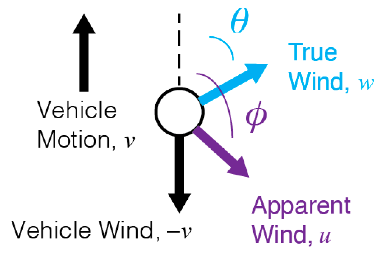
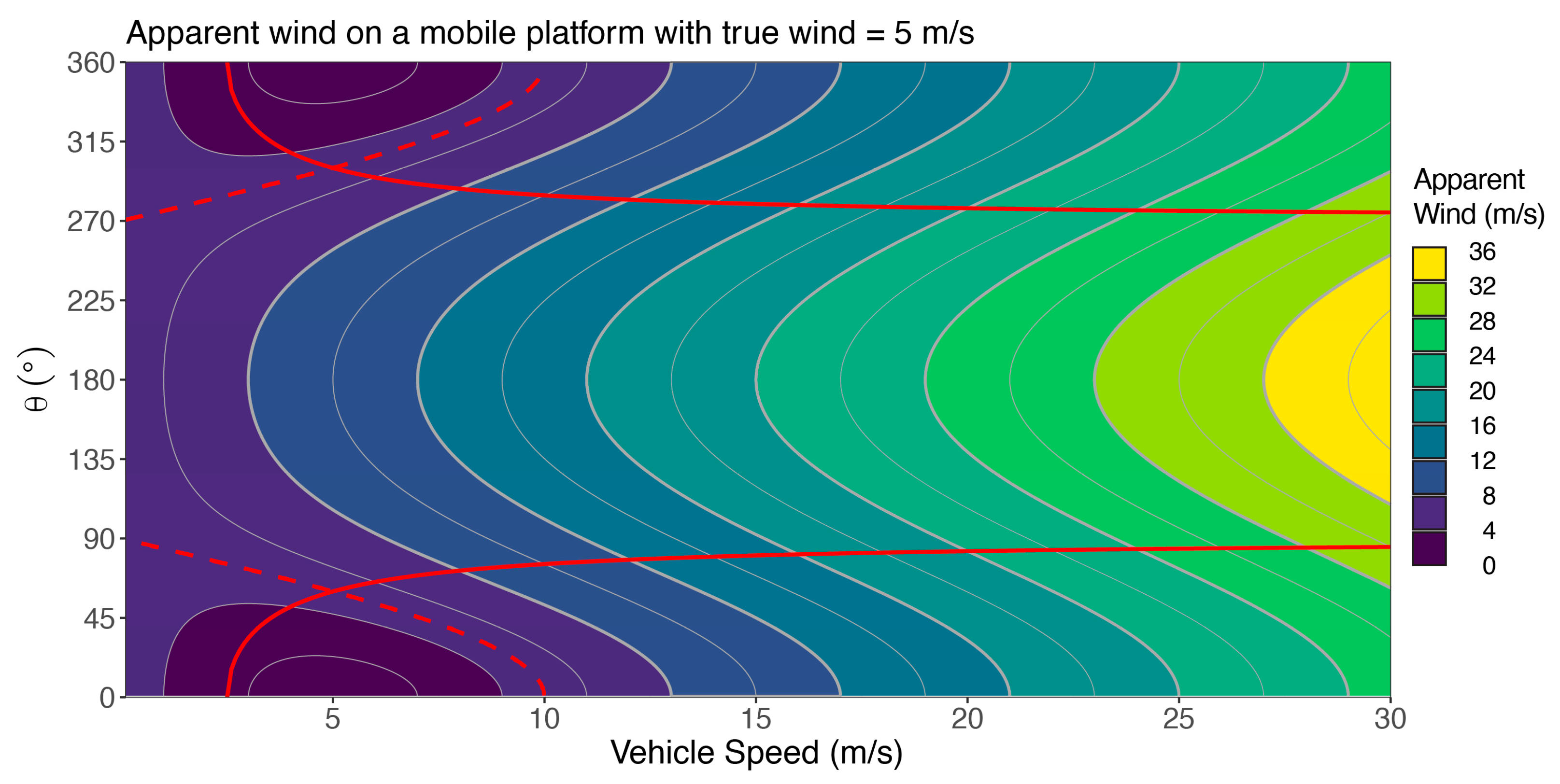
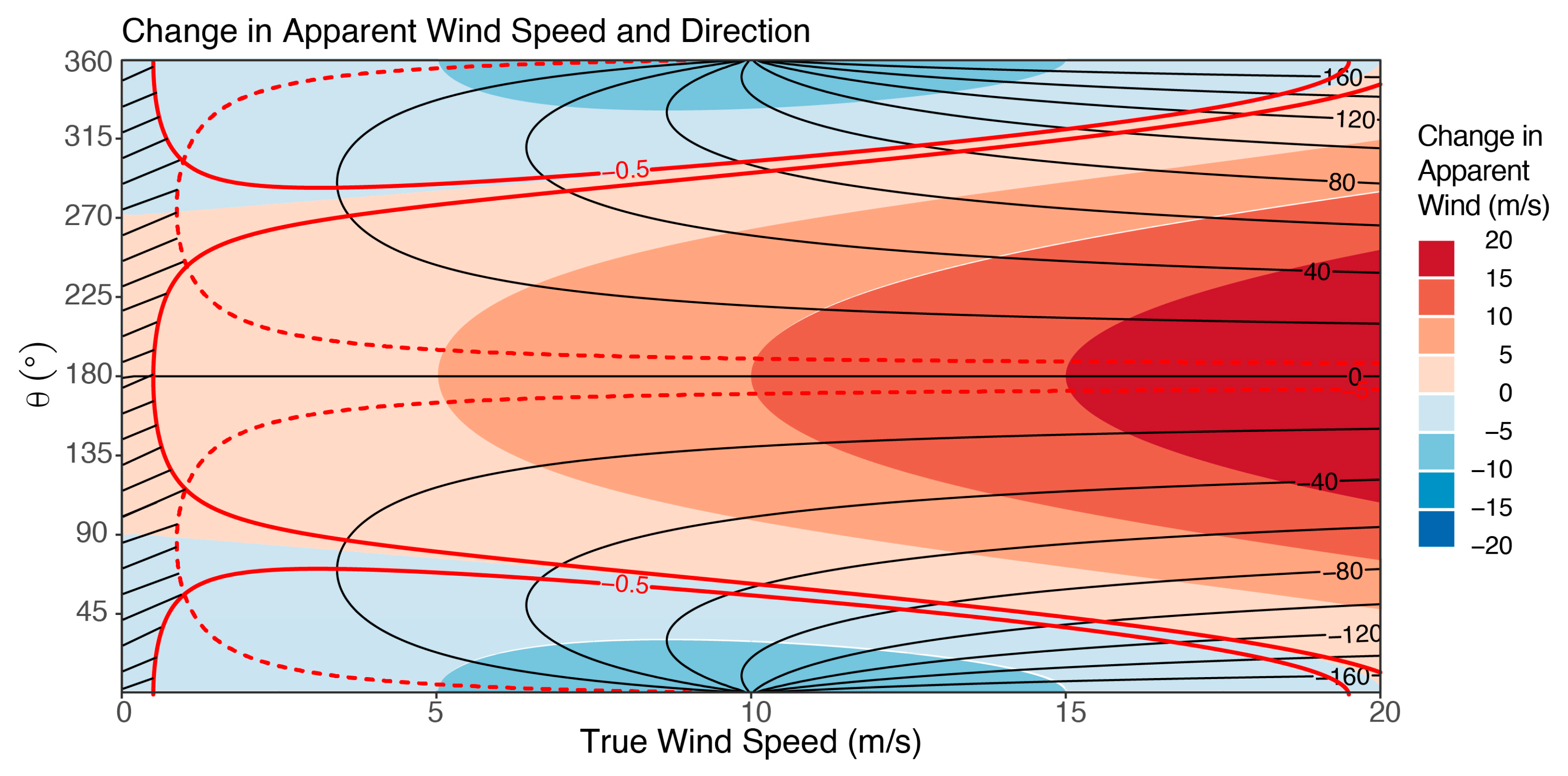
3.1. Distinguishing True Wind from Apparent Wind

The ultimate goal in mobile wind measurement is to estimate both the true wind speed and direction. A true wind is only uniquely detectable if the resulting change in the apparent wind and direction differ from the vehicle’s motion beyond the accuracy limitations of the anemometer. Otherwise, the signal of the moving vehicle dominates and obfuscates $\overrightarrow{w}$. Both the apparent wind speed and direction are required since Equation (5) allows ambiguity in the values of $u$ and $\varphi$ in determining $w$ and $\theta$. However, $u$ and $\varphi$ provide complementary pieces of information that can overcome a small change in one of the measurements. For example, a vehicle moving 10 m/s within a true wind field of 5 m/s, 75.5° off of the direction of vehicle motion will measure an apparent wind of 10 m/s, 151°. A change in wind speed is not distinguishable; however, the information within the complementary apparent wind direction constrains the true wind to its correct magnitude and orientation. This turns out to be a feature of mobile wind observation not available in a stationary environment. The motion of the vehicle and change in angle jointly provide a powerful constraint. However, issues arise when the apparent wind speed and direction both provide relatively small amounts of information, resulting in large uncertainty in true wind estimation, or even the inability to distinguish its presence.

Figure 3 shows the calculated change in apparent wind speed (filled contours) and direction (black contours) for a vehicle moving at 10 m/s for varying combinations of true wind speed ($w$) and orientation ($\theta$). As expected, the greatest changes occur for larger true wind oriented with ($\theta =0°$) or against ($\theta =180°$) the vehicle’s motion, and for the strongest true winds.

The true wind is not distinguishable if it creates changes in both $u$ and $\varphi$ that are less than the accuracy limits of the anemometer. Otherwise, within uncertainty, $u=v$ and $\varphi =180°$. As an example, we apply the anemometer accuracy limitations of the Airmar 200WX (Airmar Technology Corporation, Milford, NH, USA), a popular model with accuracy of 5% for wind speed and 3° for wind direction [25]. Additional calculations using differing accuracy ratings are straightforward. The calculations that follow are theoretical and represent simulated observations for various vehicle speeds, wind orientations to the vehicle’s motion, and true wind speeds.

Figure 3 highlights the domain of indistinguishable true wind using black hatching, enclosed by the red solid lines ($\Delta u=0.05v$; 5% of vehicle velocity) and red dashed lines ($\Delta \varphi =5°$). The accuracy of wind speed restricts observable changes only at lower values of true wind, but fingers of undetectable, small changes in apparent wind speed follow the $\Delta u=0$ contour ($u=v$) through higher true wind speeds (similar to the solid red lines in Figure 1). Winds moving parallel to the motion of the vehicle are most easily measured since the vehicle and true wind are simply additive. In these directions, the required true wind speed to become detectable depends on vehicle speed. The threshold for detection matches the wind speed accuracy, in this example 5%. In Figure 3, with $v=10 \mathrm{m}/\mathrm{s}$, this amounts to $w=0.5 \mathrm{m}/\mathrm{s}$, a modest wind. A larger true wind is required to overcome the $\cos \theta$ dependence of the apparent wind speed as the direction veers away from the parallel and antiparallel directions. The minimum speed for detectability increases as it follows the solid red contour until intersecting the red dashed contour in Figure 3. At these crossover points, the minimum value to distinguish the true wind is $w=0.10v$. This threshold remains about 10% for all vehicle speeds. The accuracy limitations of the anemometer wind speed are the most constraining factor between $\theta =302° \mathrm{t}\mathrm{o} 58° \mathrm{a}\mathrm{n}\mathrm{d} \theta =116° \mathrm{t}\mathrm{o} 244°$.

Figure 3 shows that the complementary roles of apparent wind speed and direction have shifting contributions in determining the minimum distinguishable true wind. Between $\theta =58° \mathrm{t}\mathrm{o} 116°$ and $\theta =244° \mathrm{t}\mathrm{o} 302°$, it is the uncertainty in wind direction that most constrains true wind measurement, even overcoming the uncertainty fingers of small change in $u$ starting at $\theta =90°; 270°$. The apparent wind direction changes the most for large true wind and the magnitude of the change increases from a minimum of zero ($\theta =180°$) when the wind is antiparallel to the vehicle’s motion to a maximum when it is parallel ($\theta =0°$). A change of at least $5°$ is highlighted by the red dashed contour in Figure 3. The minimum threshold, occurring at $\theta =90°; 270°$, occurs when $w=0.85 \mathrm{m}/\mathrm{s}$ for the conditions in Figure 3, but more generally can be expressed as:

$$w_{min}=v{\left(\frac{1}{{\cos }^2(180°+{\alpha }_{\varphi })}-1\right)}^{1/2}$$

(10)

where ${\alpha }_{\varphi }$ is the anenometer uncertainty in wind direction observation in degrees.

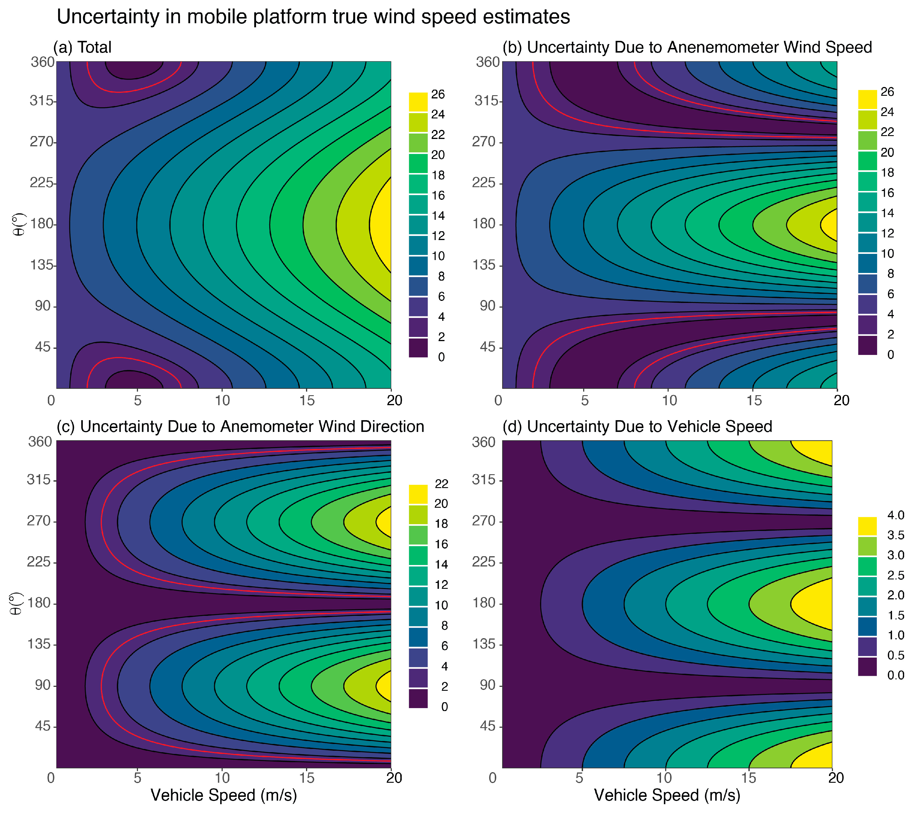
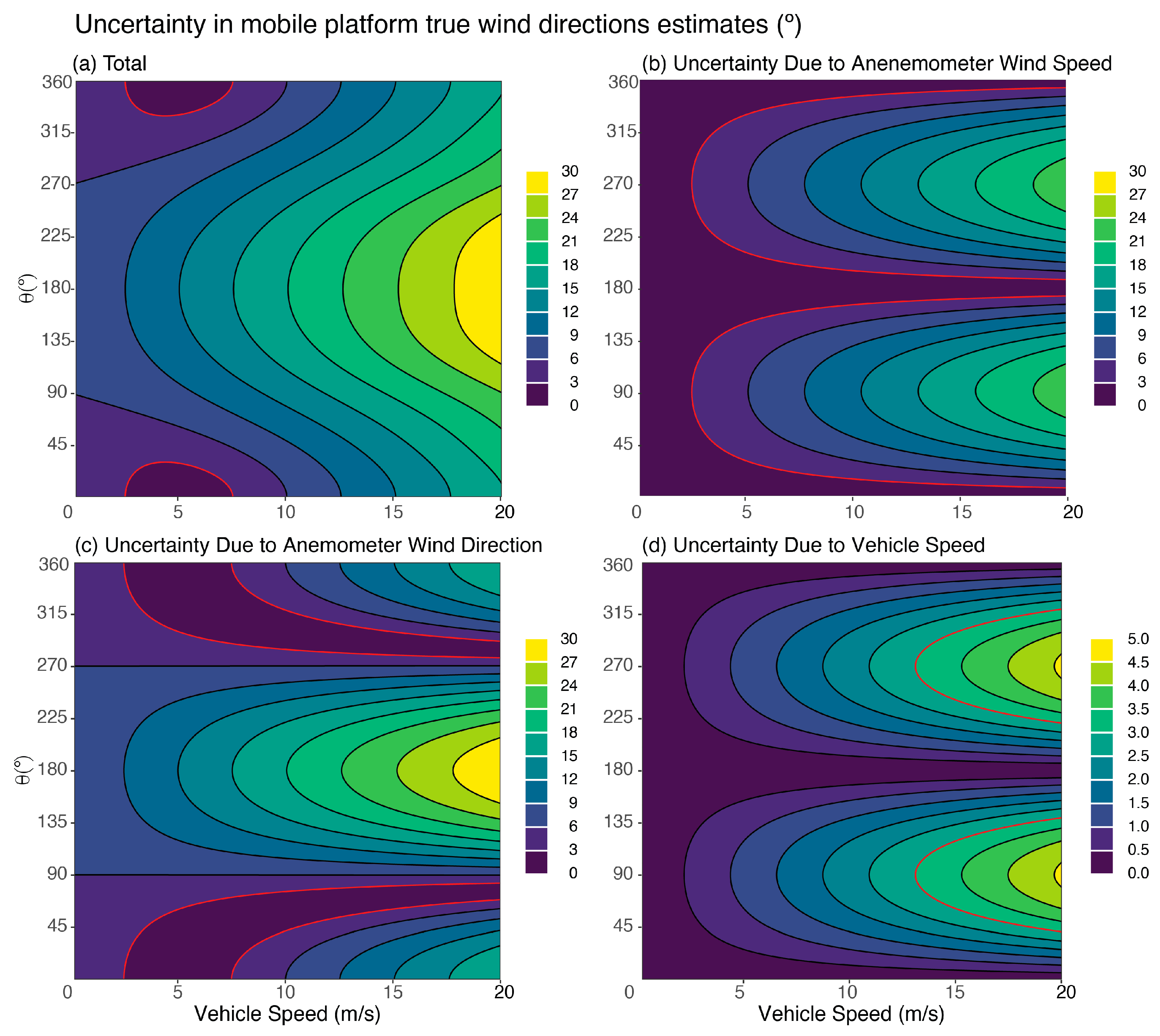
3.2. Uncertainty in True Wind Estimation

The uncertainty in estimating the true wind ($w$) is a separate issue from detectability as described in Section 3.1 and requires the propagation of error [30] from the measurement of the apparent wind speed ($u$), apparent wind direction ($\varphi$), and vehicle speed ($v$). Propagation of these three sources of uncertainty through Equation (6) leads to:

$$\begin{array}{c}\delta w=\sqrt{{\left(\frac{\partial w}{\partial u}\delta u\right)}^2+{\left(\frac{\partial w}{\partial v}\delta v\right)}^2+{\left(\frac{\partial w}{\partial \varphi }\delta \varphi \right)}^2}\hfill \\ =\frac{1}{w}\sqrt{{\left(u+v\cos \varphi \right)}^2\delta u^2+{\left(v+u\cos \varphi \right)}^2\delta v^2+u^2{v}^2{\sin }^2\varphi \delta {\varphi }^2}\hfill \end{array}$$

(11)

which shows that the uncertainty, in absolute terms, decreases with greater true wind speed and has a complicated dependence on $\varphi$ (and thus $\theta$). Note that for stationary conditions, $\delta w=\delta u$, as would be expected.

Figure 4a shows the fractional error in estimating a true wind of 5 m/s as calculated for various vehicle speeds and apparent wind directions. As in Section 3.1, the conservative but real error estimates of the Airmar 200WX are assumed, including an accuracy of 5% for the observed wind speed, 1% for the vehicle’s speed, and 3$°$ for the observed wind direction. The resulting pattern mimics the apparent wind distribution shown in Figure 2 since the uncertainty is proportional to the wind speed observed by the anemometer. The red contour highlights 5% uncertainty, the intrinsic accuracy of the anemometer. There are pockets of reduced uncertainty, even lower than the anemometer’s accuracy rating, for vehicle speeds close to the true wind speed and moving with the wind. Figure 2 shows that moving with the wind provides the lowest apparent winds and Figure 4 shows that this results in the lowest uncertainty for all vehicle speeds. In contrast, when moving into the wind, the apparent wind speed is at its greatest, as is the associated uncertainty. Outside of the pockets of low uncertainty, the magnitude of the uncertainty increases linearly with vehicle speed for each $\theta$, approximately 0.1% per m/s.

Figure 4b–d shows the contributions to the total uncertainty from the measurement of the apparent wind speed, apparent wind direction, and vehicle speed. Similar to Section 3.1, the apparent wind speed and direction play complementary roles in creating the overall pattern in Figure 4a. Figure 4b shows that the uncertainty in measuring the wind speed (anemometer error) creates hot spots where $\theta =0° \mathrm{a}\mathrm{n}\mathrm{d} 180°$ and the apparent wind is strongest. Finer structure occurs as fingers of low uncertainty, following the $u=v$ contour as previously noted in Figure 2. In these regions, the lower apparent wind speed suppresses uncertainty. The uncertainty contribution from the apparent wind direction (Figure 4c) fills these lower-uncertainty regions to make the structure of the total uncertainty (Figure 4a) smoother and closer to Figure 2. The uncertainty due to error in wind direction peaks at the crosswinds, $\theta =90°; 270°$, following the $\sin \left(\right)$ dependence of Equation (11) and highlighting the region of greatest sensitivity of $w$ to $\varphi$ (largest $\partial w/\partial \varphi$). Finally, the role of the vehicle speed is small in this example but adds to the uncertainty in the parallel and antiparallel wind directions, where it is most effective at impacting both $u$ and the determination of $w$.

The uncertainty in the true wind direction is explored using:

$$\delta \theta =\sqrt{{\Delta \theta }_u^2+{\Delta \theta }_v^2+{\Delta \theta }_{\varphi }^2}$$

(12)

where ${\Delta \theta }_u^2$, ${\Delta \theta }_v^2$, and ${\Delta \theta }_{\varphi }^2$ are the changes in $\theta$ due to the range of possible values of $u,v, \mathrm{and} \varphi$, respectively, as determined by their uncertainty. Equation (12) is conceptually similar to Equation (11) but uses iterative calculations of $\theta$ given the uncertainty ranges of $u$, $v$, and $\varphi$ to map out the extent of changes in $\theta$ rather than calculating an analytical derivative; analytical solutions containing inverse trigonometric functions tend to create unrealistic discontinuities.

Figure 5a shows the uncertainty in estimating the direction of a true wind of 5 m/s for various vehicle speeds and apparent wind directions. We again assume an accuracy of 5% for the observed wind speed, 1% for the vehicle’s speed, and 3$°$ for the observed wind direction. The distribution in Figure 5a is very similar to the pattern in Figure 2, with higher uncertainty occurring for faster true winds that flow against the motion of the vehicle. Once again, there are regions of reduced uncertainty centered on a vehicle speed matching the true wind and flow moving with the vehicle. The magnitude of the uncertainty increases nearly linearly within the vehicle speed range displayed in Figure 5, with $\theta$ increasing by 0.2$°$ per m/s increase in speed.

Figure 5b–d shows the contributions to the total uncertainty. Wind speed and direction once again play complementary roles as the total uncertainty is composed, although here their geometric distribution is flipped as compared to the wind speed. In this anemometer configuration, the uncertainty in wind direction is primarily driven by the uncertainty of observed wind speed and direction. The largest impact of wind speed uncertainty is on crosswinds, while accuracy limitations of measuring wind direction most significantly affect winds moving against the vehicle’s motion. The scale of the uncertainty range can be large, upwards of 30$°$ for a fast-moving survey.

Wind observations are arguably most important when transecting across a plume. Under these conditions, $\theta =90°$ or $270°$. The results of Figure 4 and Figure 5 suggest that improvements in both anemometer speed and direction accuracy are the most effective way to enhance cross-vehicle true wind estimation. In particular, the duality of the speed and direction splits the contributions: improving anemometer wind speed accuracy improves crosswind direction determination, while improving anemometer wind direction accuracy improves crosswind wind speed estimation.

The results in Figure 4 and Figure 5 show that the total uncertainty structure of estimating true wind speed and direction is composed primarily of the error in observed wind speed and direction with the error in vehicle speed, although with varying importance depending on wind direction relative to the vehicle. However, the structure of total uncertainty in true wind can vary dramatically if the relative amounts of error in the observed components shift. For example, Figure 6 shows that the fingers of low uncertainty in the estimated wind direction remain visible when the anemometer’s wind speed accuracy is improved. In such a case, the angle of incidence of the wind becomes even more important, but the error in crosswind also diminishes. To account for this strict dependence on the characteristics of applied anemometer and GPS unit, uncertainty analyses should be recreated for each mobile lab setup to best understand the uncertainty in true wind estimation.

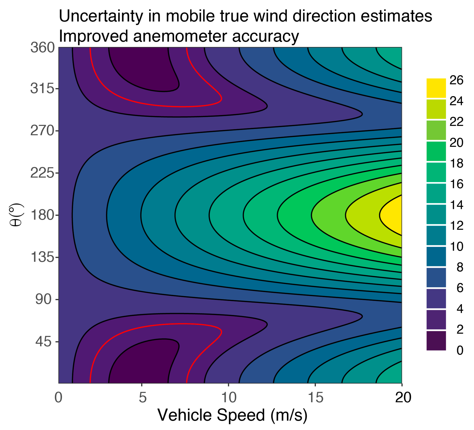
3.3. Additional Sources of Uncertainty

The uncertainty described in Section 3.2 includes the cascading effects of error in measuring $u,v, \mathrm{and} \varphi$. However, the true wind direction estimate resulting from Equation (9) is relative to the moving vehicle. The vehicle’s heading must be added to achieve the true wind with respect to true (or magnetic) north. Errors in heading are commonly of the order of 2–5° and, by error propagation [30], must simply be added on top of the uncertainty estimated in Section 3.2. Additional sources of error can arise from poorly calibrated or misaligned compasses. Indeed, an important check is to confirm that the vehicle heading, as determined by the sensor’s compass, and GPS-based course over ground are parallel. The heading and course will differ for boat or flight-based observations due to crosswinds or currents, but should match exactly for a ground-based vehicle. As a point of caution, headings and tracks are slow to respond and inaccurate during quick or frequent turns, or in locations with poor GPS reception, such as urban corridors and roads with a thick tree canopy. Care must be taken to isolate observations not meeting quality control.

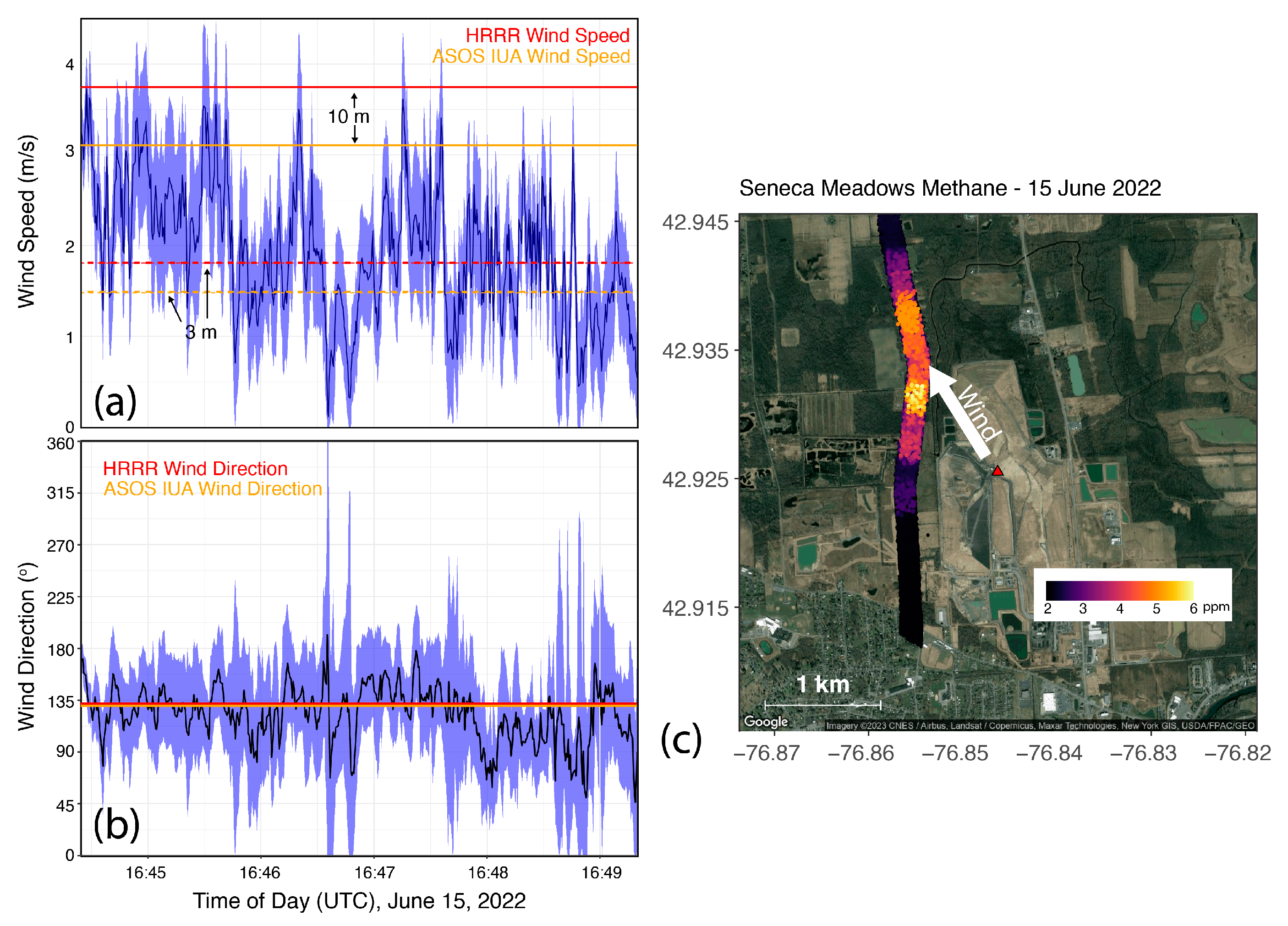
3.4. Example—Transect across a Plume

Figure 7 shows an example transect across a methane plume originating from the Seneca Meadows Landfill in Waterloo, NY, USA. Observations were collected from a Dodge Caravan containing a LICOR 7800 (methane, carbon dioxide, and water vapor), Aeris MIRA Ultra (methane, ethane, water vapor), an Airmar 200WX multiparameter weather sensor, and GPS units that provided vehicle position, track, and timing. The Airmar 200WX uses an ultrasonic anemometer with specified accuracy of 5% for wind speed and 3° for wind direction. The air inlet and meteorological observations were mounted 3 m above the ground level on a 1 m mast attached to the roof rack. The plume from the landfill is apparent in Figure 7. The mobile van was driven at 15 m/s along the western, downwind face of the landfill during this transect across the plume.

Figure 7 compares the estimated true wind with the nearby Automated Surface Observing Systems (ASOS) [31] site at the airport in Canandaigua, NY, USA, 38 km west of the landfill, which reported winds of 3.1 m/s from 130°. Similarly, output archived from the High-Resolution Rapid Refresh (HRRR) [32] weather forecast model simulates a wind of 3.8 m/s from 132°. Figure 7 shows that the wind direction is consistent across all three sources, while the mobile wind speeds are lower. However, both HRRR and ASOS report winds at 10 m and the mobile observations were collected at 3 m above ground level. The three wind values are consistent if the HRRR and ASOS values are reduced to an elevation of 3 m using a logarithmic wind profile with the closed landscape characteristic of the environment around Seneca Meadows [33]. The uncertainty analyses presented in Section 3.2 and Section 3.3 are quickly adaptable to provide error estimates for observational time series (1 Hz in this example).

Figure 7 shows the uncertainty in estimating the true wind speed and direction as blue shading. The error in wind speed was calculated for the time series by applying Equation (11) for each observation. The error in wind direction was estimated by iteratively calculating $\theta$ for the maximum and minimum potential values of $u,v,$and $\varphi$, and using the change in $\theta$ and $\delta \theta$, in Equation (12). While the average values from the mobile platform compare well with HRRR and ASOS observations, the degree of error is quite large, particularly in wind direction. Uncertainty in conditions as in Figure 7 depend greatly on the specifications of the anemometer. Reduced error can be achieved if a different anemometer with improved accuracy ratings is used (changing properties of $u$ and $\varphi$ or reduced speed (lower $v$ in Figure 4 and Figure 5)).

4. Conclusions

We have presented uncertainty characteristics in the measurement of wind speed from a mobile platform, assessing two complementary aspects: the detectability of a true wind and the associated uncertainty of a successful measurement. We also apply the uncertainty analysis to a sample set of observations to reveal utility. Wind speed and direction play prominent roles in determining chemical source and transport [5], and a proper characterization of measurements is important to reduce error and misinterpretation. The prevalence of meteorological sensors on mobile air quality laboratories and drones underscores the utility of wind measurements.

A moving anemometer creates an environment where the information contained in both the wind speed and direction can be used to constrain the true wind. Because of this complementarity, improving wind observations can be tackled with improvements in either component. However, the accuracy of the observed apparent wind speed is most directly related to the estimates of true winds that align with the vehicle’s motion, while the accuracy of the wind direction better informs about true winds moving across the vehicle.

Detectability, the condition that measurements of the apparent wind differ from the vehicle’s motion beyond the anemometer’s accuracy rating, is a relatively low bar to pass in most conditions. In the example discussed in Section 3.1, a vehicle moving at 10 m/s with an anemometer similar in specification to the Airmar 200WX would require a true wind greater than 0.5–0.9 m/s to be detectable. The range arises from the important dependence on the angle of incidence of the true wind relative to the motion of the vehicle. The higher thresholds occur when the wind is moving across the vehicle, an inconvenient result considering the usefulness of downwind transects across a plume. However, this can be counteracted by using an anemometer with greater accuracy. Indeed, all of the uncertainty discussed here can be reduced with improved anemometer accuracy ratings.

Uncertainty arising from the anemometer-measured wind speed and direction, as well as the vehicle speed, create varying degrees of error in the estimated true wind speed and direction. The uncertainty of an estimated true wind speed and direction depends not only on the error characteristics of the quantities, but also crucially on the angle of the wind relative to the vehicle motion. Uncertainty is greatest when the wind moves against the motion of the vehicle and smallest when the wind moves with the vehicle. In all cases, the uncertainty grows as vehicle speed increases. The contribution of the uncertainty in anemometer-based wind speed and direction also depends on the angle of the true wind.

In general, threshold values and true wind estimate uncertainties should be constructed for each mobile lab setup, as anemometers and GPS units have varying accuracy levels. The detectability and uncertainty characteristics described here provide modest constraints in most mobile conditions (driving < 15 m/s). However, additional sources of error, especially time lags and inaccuracies of GPS positioning when turning quick, as well as the loss of GPS signal in forested or urban canyons, are much harder to quantify and are transient. As a result, a stationary anemometer, properly oriented and calibrated, provides an important reference point that should not be overlooked.

References

1. Belušić, D.; Lenschow, D.H.; Tapper, N.J. Performance of a mobile car platform for mean wind and turbulence measurements. Atmos. Meas. Tech. 2014, 7, 1825–1837. [Google Scholar] [CrossRef]
2. Miller, S.J.; Gordon, M.; Staebler, R.M.; Taylor, P.A. A Study of the Spatial Variation of Vehicle-Induced Turbulence on Highways Using Measurements from a Mobile Platform. Boundary-Layer Meteorol. 2019, 171, 1–29. [Google Scholar] [CrossRef]
3. De Boer, G.; Waugh, S.; Erwin, A.; Borenstein, S.; Dixon, C.; Shanti, W.; Houston, A.; Argrow, B. Measurements from mobile surface vehicles during the Lower Atmospheric Profiling Studies at Elevation—A Remotely-piloted Aircraft Team Experiment (LAPSE-RATE). Earth Syst. Sci. Data 2021, 13, 155–169. [Google Scholar] [CrossRef]
4. Miller, S.J.; Gordon, M. The measurement of mean wind, variances, and covariances from an instrumented mobile car in a rural environment. Atmos. Meas. Tech. 2022, 15, 6563–6584. [Google Scholar] [CrossRef]
5. Caulton, D.R.; Li, Q.; Bou-Zeid, E.; Fitts, J.P.; Golston, L.M.; Pan, D.; Lu, J.; Lane, H.M.; Buchholz, B.; Guo, X.; et al. Quantifying uncertainties from mobile-laboratory-derived emissions of well pads using inverse Gaussian methods. Atmos. Chem. Phys. 2018, 18, 15145–15168. [Google Scholar] [CrossRef]
6. Zhang, J.; Ninneman, M.; Joseph, E.; Schwab, M.J.; Shrestha, B.; Schwab, J.J. Mobile laboratory measurements of high surface ozone levels and spatial heterogeneity during LISTOS 2018: Evidence for sea breeze influence. J. Geophys. Res.-Atmos. 2019, 124, e2019JD031961. [Google Scholar] [CrossRef]
7. Catena, A.M.; Zhang, J.; Commane, R.; Murray, L.T.; Schwab, M.J.; Leibensperger, E.M.; Marto, J.; Smith, M.L.; Schwab, J.J. Hydrogen Sulfide Emission Properties from Two Large Landfills in New York State. Atmosphere 2022, 13, 1251. [Google Scholar] [CrossRef]
8. Boanini, C.; Mecca, D.; Pognant, F.; Bo, M.; Clerico, M. Integrated Mobile Laboratory for Air Pollution Assessment: Literature Review and cc-TrAIRer Design. Atmosphere 2021, 12, 1004. [Google Scholar] [CrossRef]
9. Majluf, F.Y.; Krechmer, J.E.; Daube, C.; Knighton, W.B.; Dyroff, C.; Lambe, A.T.; Fortner, E.C.; Yacovitch, T.I.; Roscioli, J.R.; Herndon, S.C.; et al. Mobile Near-Field Measurements of Biomass Burning Volatile Organic Compounds: Emission Ratios and Factor Analysis. Environ. Sci. Technol. Lett. 2022, 9, 383–390. [Google Scholar] [CrossRef]
10. Shah, A.; Allen, G.; Pitt, J.R.; Ricketts, H.; Williams, P.I.; Helmore, J.; Finlayson, A.; Robinson, R.; Kabbabe, K.; Hollingsworth, P.; et al. A Near-Field Gaussian Plume Inversion Flux Quantification Method, Applied to Unmanned Aerial Vehicle Sampling. Atmosphere 2019, 10, 396. [Google Scholar] [CrossRef]
11. Viatte, C.; Lauvaux, T.; Hedelius, J.K.; Parker, H.; Chen, J.; Jones, T.; Franklin, J.E.; Deng, A.J.; Gaudet, B.; Verhulst, K.; et al. Methane emissions from dairies in the Los Angeles Basin. Atmos. Chem. Phys. 2017, 17, 7509–7528. [Google Scholar] [CrossRef]
12. Golston, L.M.; Pan, D.; Sun, K.; Tao, L.; Zondlo, M.A.; Eilerman, S.J.; Peischl, J.; Neuman, J.A.; Floerchinger, C. Variability of Ammonia and Methane Emissions from Animal Feeding Operations in Northeastern Colorado. Environ. Sci. Technol. 2020, 54, 11015–11024. [Google Scholar] [CrossRef]
13. Atherton, E.; Risk, D.; Fougère, C.; Lavoie, M.; Marshall, A.; Werring, J.; Williams, J.P.; Minions, C. Mobile Measurement of Methane Emissions from Natural Gas Developments in Northeastern British Columbia, Canada. Atmos. Chem. Phys. 2017, 17, 12405–12420. [Google Scholar] [CrossRef]
14. Hoesly, R.M.; Smith, S.J.; Feng, L.; Klimont, Z.; Janssens-Maenhout, G.; Pitkanen, T.; Seibert, J.J.; Vu, L.; Andres, R.J.; Bolt, R.M.; et al. Historical (1750–2014) anthropogenic emissions of reactive gases and aerosols from the Community Emissions Data System (CEDS). Geosci. Model Dev. 2018, 11, 369–408. [Google Scholar] [CrossRef]
15. Jacob, D.J.; Turner, A.J.; Maasakkers, J.D.; Sheng, J.; Sun, K.; Liu, X.; Chance, K.; Aben, I.; McKeever, J.; Frankenberg, C. Satellite observations of atmospheric methane and their value for quantifying methane emissions. Atmos. Chem. Phys. 2016, 16, 14371–14396. [Google Scholar] [CrossRef]
16. Palmer, P.I.; Feng, L.; Lunt, M.F.; Parker, R.J.; Bösch, H.; Lan, X.; Lorente, A.; Borsdorff, T. The added value of satellite observations of methane for understanding the contemporary methane budget. Phil. Trans. R. Soc. A 2021, 379, 20210106. [Google Scholar] [CrossRef]
17. Montzka, S.A.; Dutton, G.S.; Portmann, R.W.; Chipperfield, M.P.; Davis, S.; Feng, W.; Manning, A.J.; Ray, E.; Rigby, M.; Hall, B.D.; et al. A decline in global CFC-11 emissions during 2018–2019. Nature 2021, 590, 428–432. [Google Scholar] [CrossRef] [PubMed]
18. Li, Q.; Jia, H.; Qiu, Q.; Lu, Y.; Zhang, J.; Mao, J.; Fan, W.; Huang, M. Typhoon-Induced Fragility Analysis of Transmission Tower in Ningbo Area Considering the Effect of Long-Term Corrosion. Appl. Sci. 2022, 12, 4774. [Google Scholar] [CrossRef]
19. Conley, S.; Faloona, I.; Mehrotra, S.; Suard, M.; Suard, M.; Lenschow, D.H.; Sweeney, C.; Herndon, S.; Schwietzke, S.; Pétron, G.; et al. Application of Gauss’s theorem to quantify localized surface emissions from airborne measurements of wind and trace gases. Atmos. Meas. Tech. 2017, 10, 2245–2258. [Google Scholar] [CrossRef]
20. Hanlon, T.; Risk, D. Using Computational Fluid Dynamics and Field Experiments to Improve Vehicle-Based Wind Measurements for Environmental Monitoring. Atmos. Meas. Tech. 2020, 13, 191–203. [Google Scholar] [CrossRef]
21. Yahaya, S.; Frangi, J.P. Cup Anemometer Response to the Wind Turbulence-Measurement of the Horizontal Wind Variance. Ann. Geophys. 2004, 22, 3363–3374. [Google Scholar] [CrossRef]
22. Barbieri, L.; Kral, S.T.; Bailey, S.C.C.; Frazier, A.E.; Jacob, J.D.; Reuder, J.; Brus, D.; Chilson, P.B.; Crick, C.; Detweiler, C.; et al. Intercomparison of Small Unmanned Aircraft System (sUAS) Measurements for Atmospheric Science during the LAPSE-RATE Campaign. Sensors 2019, 19, 2179. [Google Scholar] [CrossRef]
23. Thielicke, W.; Hübert, W.; Müller, U.; Eggert, M.; Wilhelm, P. Towards Accurate and Practical Drone-Based Wind Measurements with an Ultrasonic Anemometer. Atmos. Meas. Tech. 2021, 14, 1303–1318. [Google Scholar] [CrossRef]
24. Anemoment TriSonica Features. Available online: https://anemoment.com/features/ (accessed on 8 April 2023).
25. Airmar 200WX WeatherStation® Instrument Specifications. Available online: https://www.airmar.com/weather-description.html?id=154 (accessed on 7 March 2023).
26. Young, R.M. ResponseONE Ultrasonic Anemometer. Available online: https://www.youngusa.com/product/responseone-ultrasonic-anemometer/ (accessed on 7 March 2023).
27. Campbell Scientific Wind Speed and Direction. Available online: https://www.campbellsci.com/wind-speed-direction (accessed on 7 March 2023).
28. Smith, S.R.; Bourassa, M.A.; Sharp, R.J. Establishing More Truth in True Winds. J. Atmos. Ocean Technol. 1999, 16, 939–952. [Google Scholar] [CrossRef]
29. Moore, D.P.; Li, N.P.; Wendt, L.P.; Castañeda, S.R.; Falinski, M.M.; Zhu, J.-J.; Song, C.; Ren, Z.J.; Zondlo, M.A. Underestimation of Sector-Wide Methane Emissions from United States Wastewater Treatment. Environ. Sci. Technol. 2023, 57, 4082–4090. [Google Scholar] [CrossRef] [PubMed]
30. Taylor, J.R. An Introduction to Error Analysis: The Study of Uncertainties in Physical Measurements; University Science Books: Herndon, VA, USA, 1996. [Google Scholar]
31. Automated Surface Observation Systems. Available online: https://www.weather.gov/asos/ (accessed on 7 March 2023).
32. The High-Resolution Rapid Refresh Model. Available online: https://rapidrefresh.noaa.gov/hrrr/ (accessed on 7 March 2023).
33. Stull, R. Atmospheric Boundary Layer in: Meteorology: An Algebra-Based Survey of Atmospheric Science; University of British Columbia: Vancouver, BC, Canada, 2023. [Google Scholar]
Figure 1. Components of the apparent wind, u , measured aboard a moving vehicle. The motion of the vehicle creates a wind in the opposite direction, − v . The true wind w occurs at an angle θ relative to the forward motion. The resulting apparent wind, relative to the vehicle, u , is the vector sum of v and w with an orientation angle of ϕ relative to the steady motion of the vehicle.
Atmosphere 14 00765 g001
Figure 2. The apparent wind speed, u , as measured on a vehicle moving with speed v . Here, the true wind speed is 5 m/s with variable direction θ relative to a forward heading. The dashed red line indicates an apparent wind of 5 m/s, its true value. The solid red line indicates an apparent wind equal to the vehicle’s speed. Gray contours increment apparent wind speed every 2 m/s.
Atmosphere 14 00765 g002
Figure 3. The change in apparent wind speed ( u , filled contours) and direction ( ϕ , black contours) arising from a true wind with speed w and direction θ relative to the vehicle motion. Values depicted here are calculated for a vehicle moving with speed v = 10   m / s . The solid red contour highlights an apparent wind speed change of 0.5 m/s, 5% of the vehicle’s motion and the minimum change detectable by the anemometer. The dashed red contour highlights a 5 ° change in apparent wind direction, the minimum detectable change for this hypothetical anemometer. Black hatching depicts conditions indistinguishable from the motion of the vehicle.
Atmosphere 14 00765 g003
Figure 4. The fractional uncertainty (%) in the observation of a true wind of 5 m/s for varying vehicle speed and true wind direction. Panel (a) shows the total uncertainty, (b) contains the uncertainty due to the anemometer accuracy rating, (c) is the uncertainty arising from the anemometer’s wind direction, and (d) presents the uncertainty due to error in the vehicle speed. The solid red contour highlights 5% uncertainty, the accuracy of the anemometer.
Atmosphere 14 00765 g004
Figure 5. The uncertainty (°) in the estimated direction of a true wind of 5 m/s for varying vehicle speed and true wind direction. Similar to Figure 4, panel (a) shows the total uncertainty, (b) contains the uncertainty due to the anemometer’s accuracy rating, (c) is the uncertainty arising from the anemometer’s wind direction, and (d) presents the uncertainty due to error in the vehicle speed. The solid red contour highlights 3° uncertainty, the accuracy of the anemometer.
Atmosphere 14 00765 g005
Figure 6. The uncertainty in wind direction (°), similar to Figure 4 but with anemometer wind speed accuracy improved to 1%. The solid red contour highlights 5% uncertainty, the accuracy of the anemometer.
Atmosphere 14 00765 g006
Figure 7. Estimates of (a) true wind speed and (b) direction (bottom) during a pass through (c) a methane plume (right) from the Seneca Meadows Landfill in Waterloo, NY, USA. Blue shading indicates the range of uncertainty. Red lines indicate conditions extracted from HRRR forecast simulations for this period, while the orange lines show the conditions at the closest ASOS site in Canandaigua, NY, USA, 38 km west of the landfill. The HRRR and ASOS observations are reported at 10 m; the dashed line shows the extrapolated values at 3 m, the height of the mobile anemometer. The white arrow in panel (c) indicates the estimated wind direction as observed from the moving vehicle.
Atmosphere 14 00765 g007
Disclaimer/Publisher’s Note: The statements, opinions and data contained in all publications are solely those of the individual author(s) and contributor(s) and not of MDPI and/or the editor(s). MDPI and/or the editor(s) disclaim responsibility for any injury to people or property resulting from any ideas, methods, instructions or products referred to in the content.