Abstract
Surface interactions occur near the land–atmosphere interface, thus affecting the temperature, convection, boundary layer, and stability of the atmosphere. A proper representation of surface interactions is a crucial component for numerical atmospheric and air quality modeling. We assessed four land surface schemes—1. 5-layer thermal diffusion scheme (1 5-Layer); 2. unified Noah land surface model (2 Noah); 3. rapid update cycle (3 RUC) land surface model; and 4. Pleim–Xiu land surface model (4 Pleim–Xiu)—from the Weather Research and Forecasting with Chemistry (WRF-Chem V3.2) model for the purposes of atmospheric modeling in Cuenca, which is a region with a complex topography and land use configuration and which is located in the Southern Andean region, in Ecuador. For this purpose, we modeled the meteorological and air quality variables during September 2014. It was found that the meteorological and short-term air quality variables were better modeled through the 2 Noah scheme. Long-term (mean monthly) air quality variables were better modeled by the 1 5-Layer and 3 RUC options. On average, the 2 Noah scheme was better at modeling meteorology and air quality. In addition, we assessed the 2 Noah scheme combined with the urban canopy model (UCM) (5 Noah UCM), which was developed as an option to represent the urban effects at a subgrid-scale. Results indicated that the performance of the 5 Noah UCM scheme was not better at modeling than the 2 Noah scheme alone. Moreover, the 5 Noah UCM scheme notably decreased the modeling performance for carbon monoxide and fine particulate matter. These results complement previous assessments of other schemes, allowing us to recommend a basic configuration of parameters for atmospheric modeling in the Andean region of Ecuador.
1. Introduction
Surface processes occur near the land surface–atmosphere interface [1]. The movement of heat and water through this interface affects components, such as temperature, convection, boundary layer height, and stability, thus conditioning the performance of atmospheric and air quality modeling [2,3,4,5]. As solar radiation reaches the surface, a part of it is reflected, but much is absorbed. In addition, the atmosphere emits infrared radiation, thus warming the surface [6]. Energy from these two sources is stored in the soil or transferred to the atmosphere through sensible and heat fluxes. These interactions define the temperature and humidity near the ground surface and are modeled by the land surface schemes, which provide heat and moisture fluxes over the surface points. The different land surface models have various degrees of sophistication. Studies have found a high degree of variability in their results [7] and reported that surface temperature is a sensitive variable to land surface schemes [5,8]. Therefore, dedicated assessments of these land surface models are required to identify the option with the best performance for atmospheric modeling.
For modeling land surface fluxes, such as in the Weather Research and Forecasting with Chemistry model (WRF-Chem V3.2), information from the surface layer scheme, radiation, and precipitation from the microphysics and convective components, are combined with land variables and properties in order to provide an account of the heat and moisture fluxes [9].
The 5-layer thermal diffusion scheme (1 5-Layer); is a simple land surface model that is based on the MM5 five-layer soil temperature model [10]. This scheme works with five layers; below them, the temperature is fixed at a deep-layer average. The soil moisture is set with land use and season-dependent constant value, without vegetation effects. This scheme is the simplest in structure and physics when compared to the following land surface options.
The unified Noah land surface model (2 Noah) [11] is a four-layer soil temperature and moisture model with canopy moisture and snow cover prediction, as well as including the root zone, evapotranspiration, soil drainage, and runoff variables in its modeling. It also considers the influence of vegetation categories and soil texture. This scheme provides an account of the sensible and latent heat fluxes with respect to the boundary layer and has an improved urban treatment.
As default, the rapid update cycle (3 RUC) land surface scheme [12,13] works with six soil levels, solving heat diffusion and moisture transfer equations with higher resolution at the top of the soil. It includes vegetation effects and canopy water, using a layered approach to solve the energy and moisture budgets. The layer spans the ground surface, including half of the first atmospheric layer and half of the top soil layer.
The Pleim–Xiu land surface scheme (4 Pleim–Xiu) [14,15] works with a two-layer soil temperature and moisture model. This scheme considers three components for moisture: evapotranspiration, soil evaporation, and evaporation from wet canopies. The soil parameters are derived from the fractional coverages of land use categories and soil texture types.
Table 1 summarizes the main features and configuration of soil layers of these four schemes. They are coded in WRF-Chem V3.2 for modeling the land surface processes.

Table 1.
Land surface scheme options in the WRF-Chem V3.2, based on [9].
An urban canopy model (UCM) can complement a land surface scheme to consider the influence of urban areas at the subgrid-scale [1]. The UCM component parameterizes the effects of street canyons, shadowing from buildings, a wind profile in the canopy layer, and a heat model from roof and road surfaces.
In 2021, in Cuenca–a city located in the Southern of the country (Figure 1)–PM2.5 yearly mean concentrations between 5.7 to 9.8 µg m−3 were measured, which were larger than the current World Health Organization (WHO) guideline (5.0 µg m−3) [16,17]. Moreover, during forty days from 2021, the PM2.5 24 h mean levels in the historic center were higher than the current WHO guideline (15 µg m−3). In addition, the O3 levels can reach concentrations that are more elevated than the corresponding WHO guideline (100 µg m−3, maximum 8 h daily mean) [18], typically during September, which is when high levels of solar radiation reach the Ecuadorian region at the surface, promoting photochemical O3 production [19].
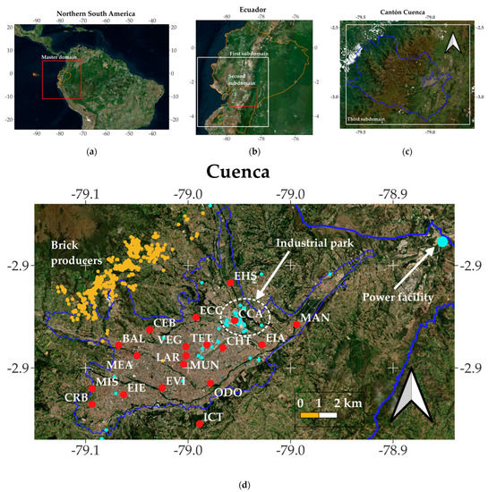
Figure 1.
Location of: (a) Ecuador and (b,c) Cantón Cuenca. (d) The urban area of Cuenca (blue border) and the air quality network from Cuenca (red dots). Nomenclature of stations: MUN, Municipio; MAN, Machángara; CEB, Cebollar; BCB, and Bomberos; ICT, Ictocruz; CRB, and Colegio Rafael Borja; MIS, Misicata; EIE, Escuela Ignacio Escandón; EVI, and Escuela Velasco Ibarra; ODO, Facultad de Odontología; LAR, Calle Larga; BAL, Balzay; MEA, and Mercado El Arenal; CHT, Colegio Herlinda Toral; VEG, Vega Muñoz; TET, and Terminal Terrestre; EIA, Escuela Ignacio Andrade; ECC, Escuela Carlos Crespi; CCA, and Colegio Carlos Arízaga; and EHS, Escuela Héctor Sempértegui. Yellow dots indicate the artisanal brick producers. Cyan dots indicate industries.
The WRF-Chem V3.2 model was used in Cuenca, which is a region with a complex topography and land use configuration, where atmospheric modeling is challenging. Emissions from the inventory of 2014 were used to assess the influence of planetary boundary layer schemes [20], as well as global atmospheric datasets [21] for modeling meteorology and air quality. For these studies, the direct effects between aerosols and meteorology were activated. This was performed because this feedback improved the performance when modeling the air quality in Cuenca [20]. However, a preliminary modeling assessment with direct and indirect effects showed no benefits for Cuenca [22]. Moreover, the 2014 emission inventory and the WRF-Chem model were used to assess the impact on air quality due to the future replacement of diesel by electrical buses [23], and to estimate the benefit on PM2.5 levels, due to the advance of combustion activities on 31 December [24]. Although the modeling performances for these studies were promising, they require improvements. For this purpose, other components, such as the land surface and urban canopy model, deserve a dedicated evaluation to improve the configuration of schemes and options for atmospheric modeling in this region.
At the time of writing this manuscript, the Municipality of Cuenca is updating the emission inventory, taking the year 2021 as its basis. One way to assess the quality of the new emission inventory will be using these results in WRF-Chem, for the purposes of modeling both meteorology and air quality during selected periods in 2021.
Therefore, the goals of this contribution are to address the following questions:
- What land surface scheme from WRF-Chem V3.2 provides the best performance for modeling the meteorological variables and air quality in Cuenca?
- Is there a benefit when considering the influence of the urban area through the urban canopy option?
- What are the recommendation for a land surface and urban canopy model to assess the quality of the in-progress emission inventory of Cuenca?
2. Methods
2.1. The Air Quality Network
To monitor meteorology and air quality, since 2012 the city has had an automatic station in the historic center (MUN station, Figure 1), at coordinates 2.89° S, 79.0° W, and 2500 masl. In addition, the air quality network has around twenty passive stations for monitoring the monthly mean concentrations of NO2 and O3 (Figure 1d). The municipality of Cuenca is the accredited entity to operate the air quality network; further, it is mandated to apply the required methods of the Ecuadorian regulations.
The study of records provided by the MUN station allowed the identification of the weekend effect (WE) in the historic center of Cuenca [23]. The WE indicates counterintuitive behavior regarding O3, which increases during weekends, although the emissions of its precursors (NOx and NMVOC) decrease.
2.2. Emission Inventory of 2014
Cuenca’s last emission inventory was built for 2014 [25]. This inventory indicates that on-road traffic was the primary source of pollutants (94.9% of CO, 71.2% of NOx, 42.4% of PM2.5, and 39.6% of NMVOC). Other NMVOC-relevant sources were found to be solvents (29.7%) and vegetation (19.5%). Industries, most of them located in the industrial park–which is in the northeast urban area (Figure 1d)–were the most significant source of SO2 (60.1%). Approximately 600 artisan brick producers (northwest, out of the urban area) generated 38.5% of the PM2.5 emissions. In addition, a thermoelectric facility (northeast, out of the urban area) generated 35.1% of SO2 and 18.5% of NOx emissions.
2.3. Modeling Approach
We used the WRF-ChemV3.2 for modeling the meteorological and air quality variables in Cuenca during September 2014. The WRF-Chem is a non-hydrostatic and Eulerian 3-D model that is used for atmospheric research and forecasting purposes [26]. It can optionally include the chemical transport of air pollutants in its modeling, thus, allowing for the use of an online approach for modeling interactions between air pollutants and meteorological variables.
Firstly, a master domain and two nested subdomains (Figure 1) were used to run the meteorological simulations. The inner subdomain is a grid of 100 × 82 cells, 1 km on each side, which covers the territory of Cuenca (Figure 1c). Table 2 details the main features of the domains.

Table 2.
Configuration of the domains for modeling the meteorology and air quality in Cuenca.
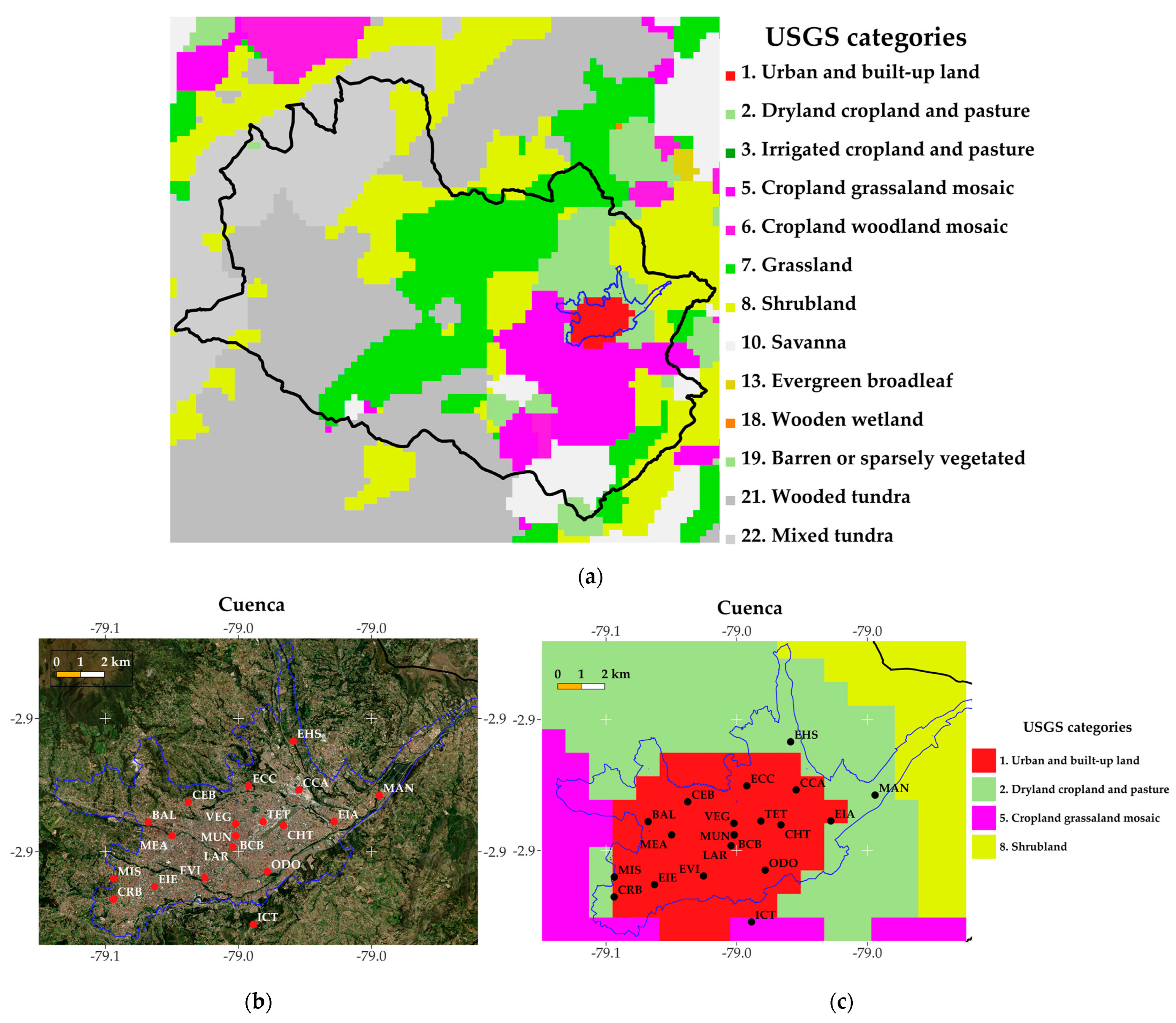
The land use maps were defined based on the US Geological Survey (USGS) categories. Figure 2 depicts the land use map for the inner domain, which indicates that cropland grassland mosaic, dryland cropland, pasture, and shrubland were the most important in terms of coverage surrounding the urban and built-up land area. Each cell was assigned a unique category based on the most abundant land use range.

Figure 2.
(a) Land use coverage (1 km of resolution) for the inner domain. Based on the US Geological Survey land use categories. (b) Zoom of the urban area. (c) Zoom of the urban area and the land use coverage for modeling.
Based on the performance of the global meteorological datasets over this region, we used the FNL Global Operational Analysis (Final), produced by the National Centers for Environmental Prediction (NCEP) [27], for generating the initial and boundary conditions. The chemical transport of pollutants option was activated for the third subdomain for the purposes of reading the hourly emissions coming from the emission inventory of Cuenca in 2014. The simulation period covers 1 to 27 September 2014, and it was focused on accounting for the high O3 levels that are typically measured during this month. The Carbon Bond Mechanism Z (CBMZ) [28] and the model for simulation aerosol chemistry and interaction (MOSAIC) were used to speciate and represent, respectively, the corresponding hourly emissions [29]. Table 3 summarizes the primary schemes and options selected for the modeling approach.

Table 3.
Main schemes and options selected for modeling the meteorology and air quality in Cuenca (WRF-Chem V3.2).
2.4. Modeling Performance
The performance for modeling surface temperature was assessed by the gross error (GE), mean (MB), and index of agreement (IOA) (Table 4). The performance for modeling wind speed was assessed by the root mean square error (RMSA), MB, and IOA. For wind direction, GE and MB were used. The expressions of these metrics are described in the EEA (2011) [39] and in the study of Simon et al. (2012) [40].

Table 4.
Metrics for modeling meteorological and air quality variables [39,40].
For short-term air quality modeling performance, we evaluated the CO (maximum mean in 1 h and 8 h, per day), PM2.5 (mean in 24 h), and O3 (maximum mean in 8 h, per day) concentrations during periods consistent with the Ecuadorian air quality legislation and the WHO guidelines [17,41]. For these variables, we used MB, RMSE, fractional bias (FB), the mean normalized bias (MNB), and the correlation coefficient (r) [40].
In addition, we obtained the percentages of records, which were captured by modeling. It was considered that a record was adequately modeled if the maximum deviation between the observed and modeled value agreed with the accuracies of Table 4. For long-term air quality (NO2 and O3), the modeling performance was considered as the percentage of the passive stations with a maximum difference of 30%.
3. Results
3.1. Meteorology
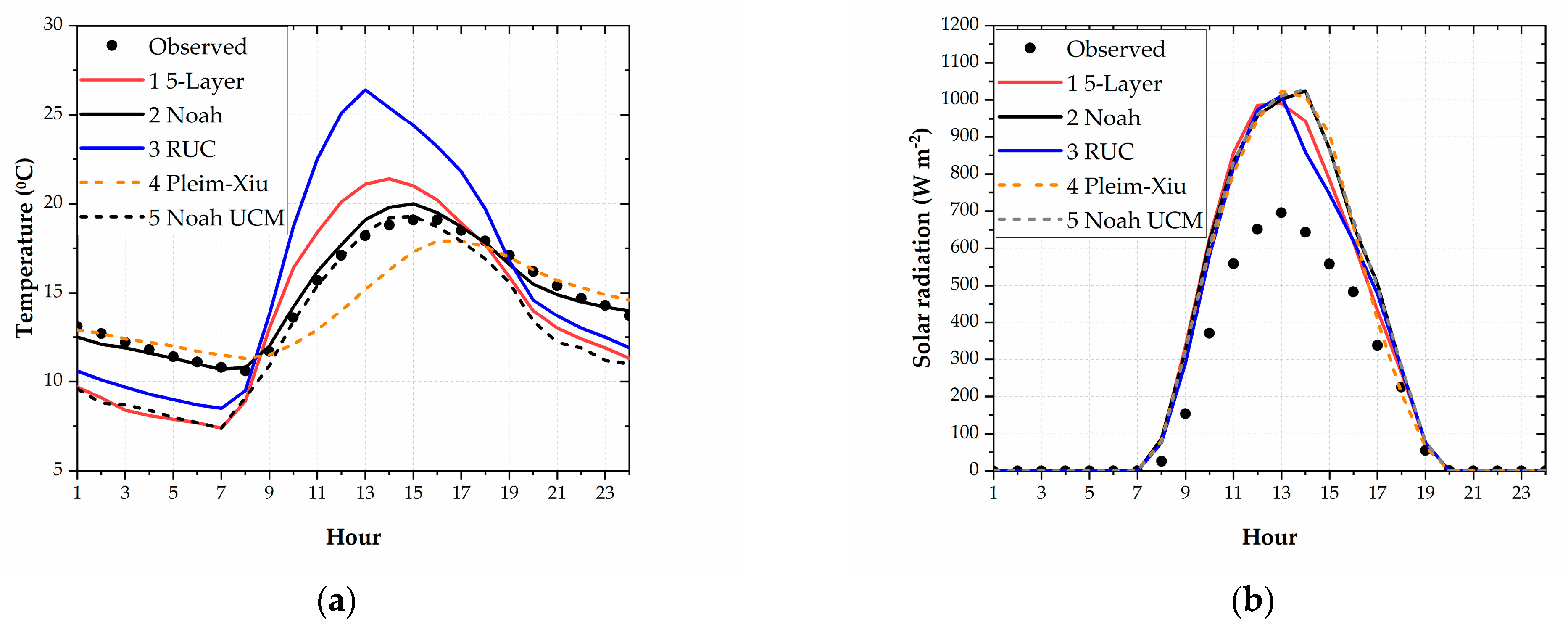
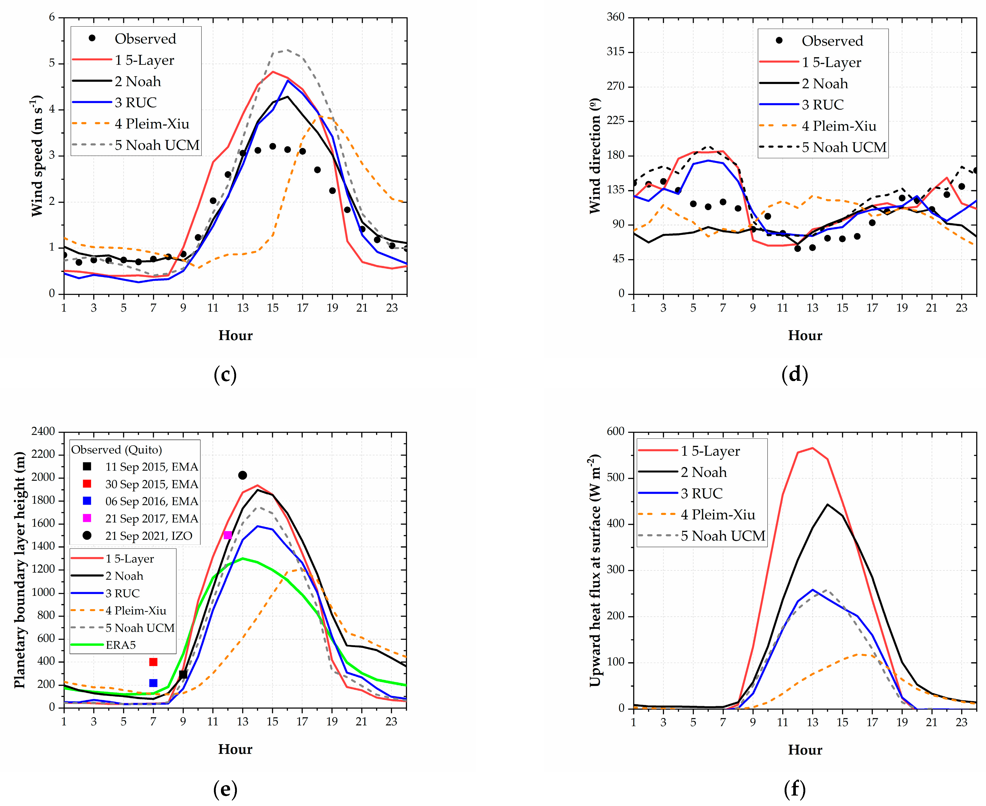
The 2 Noah land surface scheme was better when modeling surface temperature, followed by the 4 Pleim–Xiu scheme (Table 5). These options received the GE, MB, and IOA metrics into the corresponding value benchmark ranges. The 2 Noah option reproduced, in the best way, the mean daily profile (Figure 3a). On average, the 4 Pleim–Xiu option underestimated the surface temperature between 09:00 to 16:00 local time (LT) (MB = −0.5 °C). In addition, a strong relationship between measured and modeled temperatures (IOA = 0.9 and 1.0) was established for these two schemes. The 2 Noah scheme captured the highest percentage (78.0%) of the hourly temperature records (Table 6). The 1 5-Layer and 3 RUC options underestimated the temperature during the first hours of the day and then overestimated it during most of the daylight hours. The 5 Noah UCM option modeled the mean temperature profile well during the morning, as well as during the first hours of the afternoon (Figure 3a). However, this option underestimated the temperature during the hours without solar radiation.

Table 5.
Metrics for the meteorological modeling. Bold numbers indicate values in the benchmark ranges.
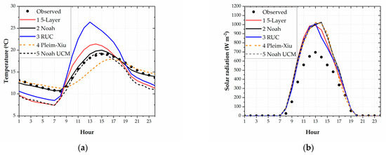
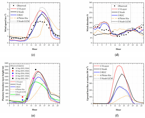
Figure 3.
Daily mean profile during September 2014 at the location of the MUN station: (a) Temperature. (b) Global solar radiation. (c) Wind speed. (d) Wind direction. (e) Planetary boundary layer height (PBLH). Squares in (e) show PBLH observations at the EMA station [42]. The black dot indicates the observation at the IZO station [43]. (f) The modeled upward heat flux at the surface by the schemes.

Table 6.
Percentages of the records that were captured by modeling. Meteorological variables. Bold numbers highlight the schemes with the best performances.
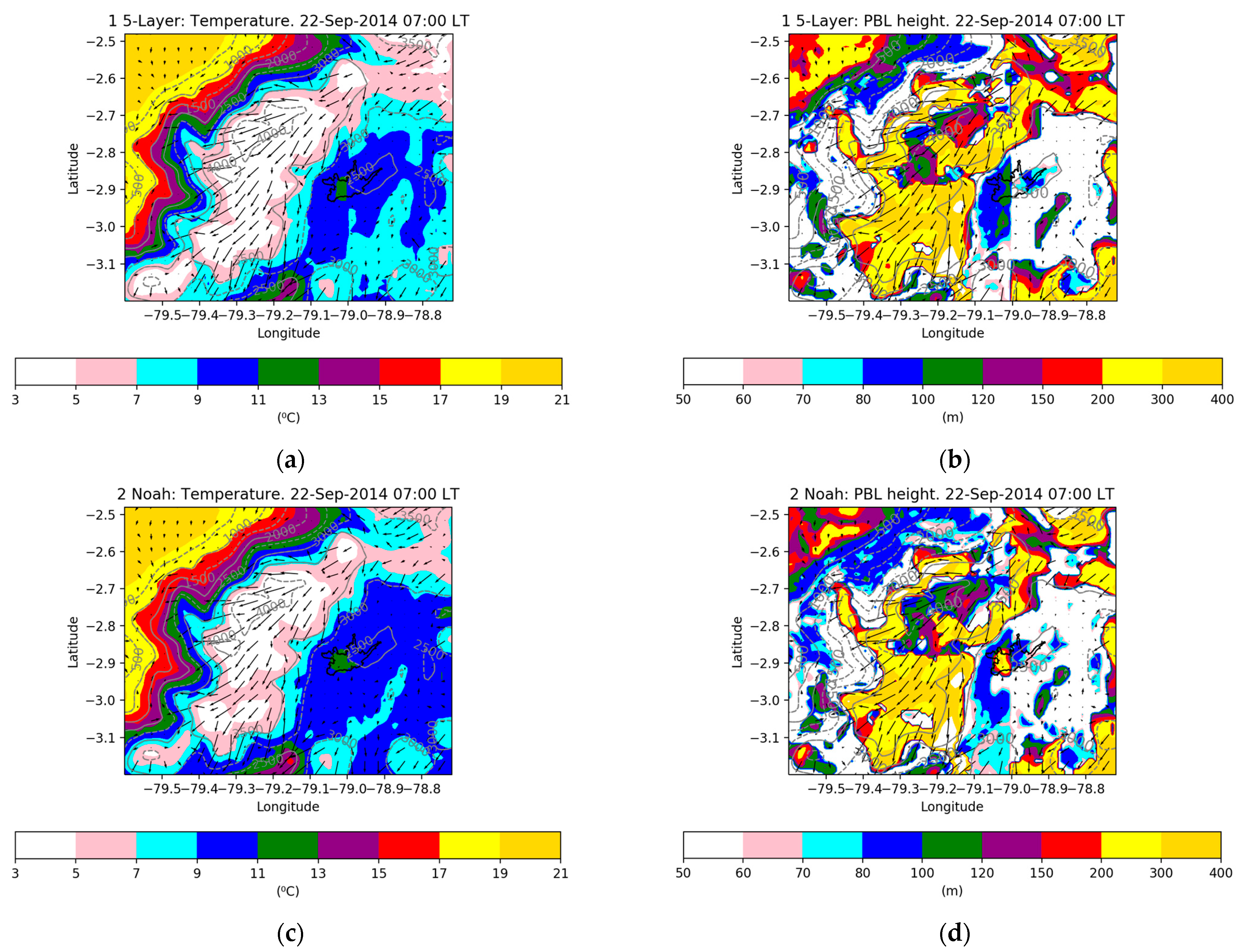
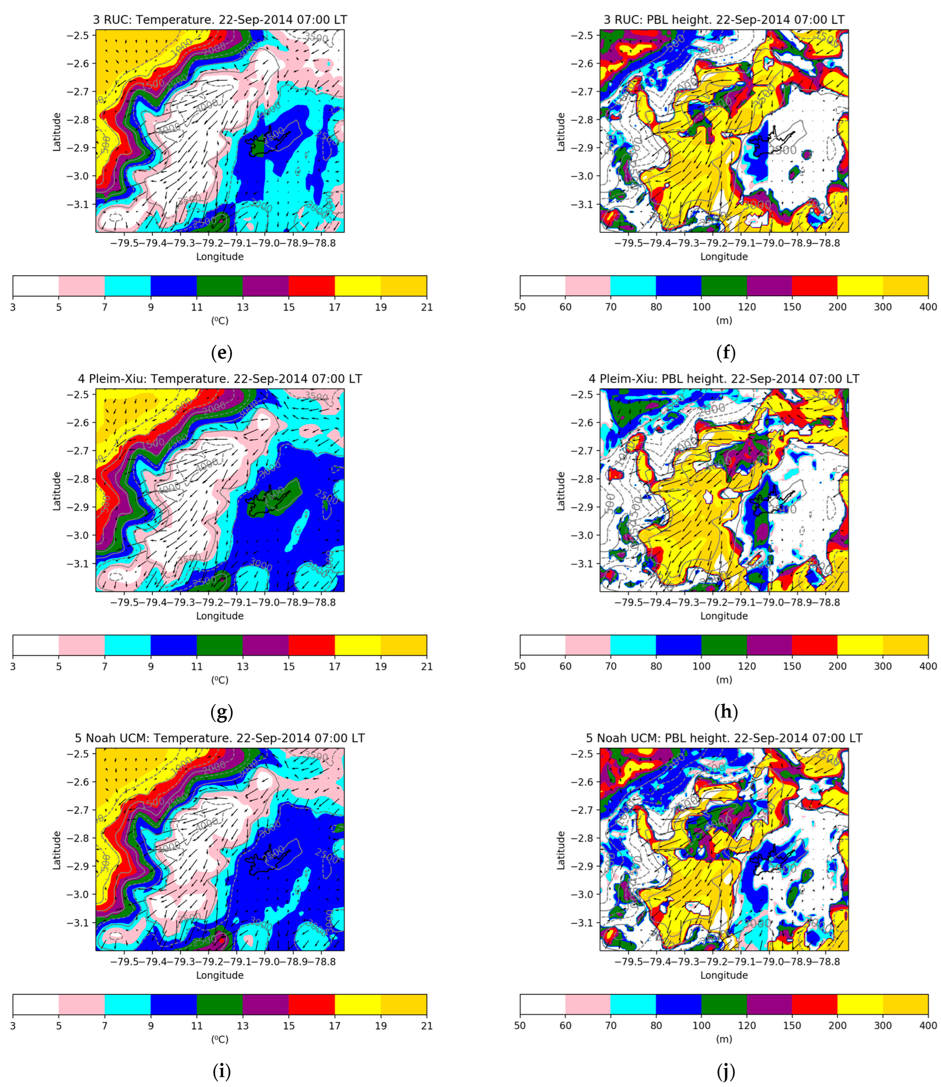
Figure 4 shows the spatial distribution of the modeled temperature on 22 September 2014, at 07:00 LT. Over the urban area, the 2 Noah option provided temperatures mostly between 11 and 13 °C. The 1 5-Layer option modeled temperatures mostly between 9 and 11 °C. The 3 RUC and 4 Pleim-Xiu schemes obtained temperatures ranging from 15–17 °C and 13–15 °C, respectively, in the complete urban area. The 5 Noah UCM option provided temperatures between 9 and 11 °C over the entire urban area. Figure 3 also shows the corresponding computed values of the planetary boundary layer heights. Over the urban area, the 2 Noah option calculated values between 70 and 300 m. The other options produced lower values, between 50 and 120 m for the 1 5-Layer and 4 Pleim–Xiu models, and between 50 and 100 m for 3 RUC and 5 Noah UCM options.
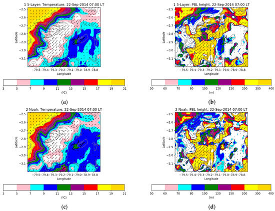
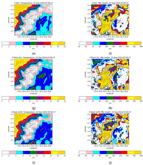
Figure 4.
Modeled temperature and planetary boundary layer height on 22 September 2014 (07:00 LT): (a,b) 1 5-Layer; (c,d) 2 Noah; (e,f) 3 RUC; (g,h) 4 Pleim–Xiu; (i,j) 5 Noah UCM.
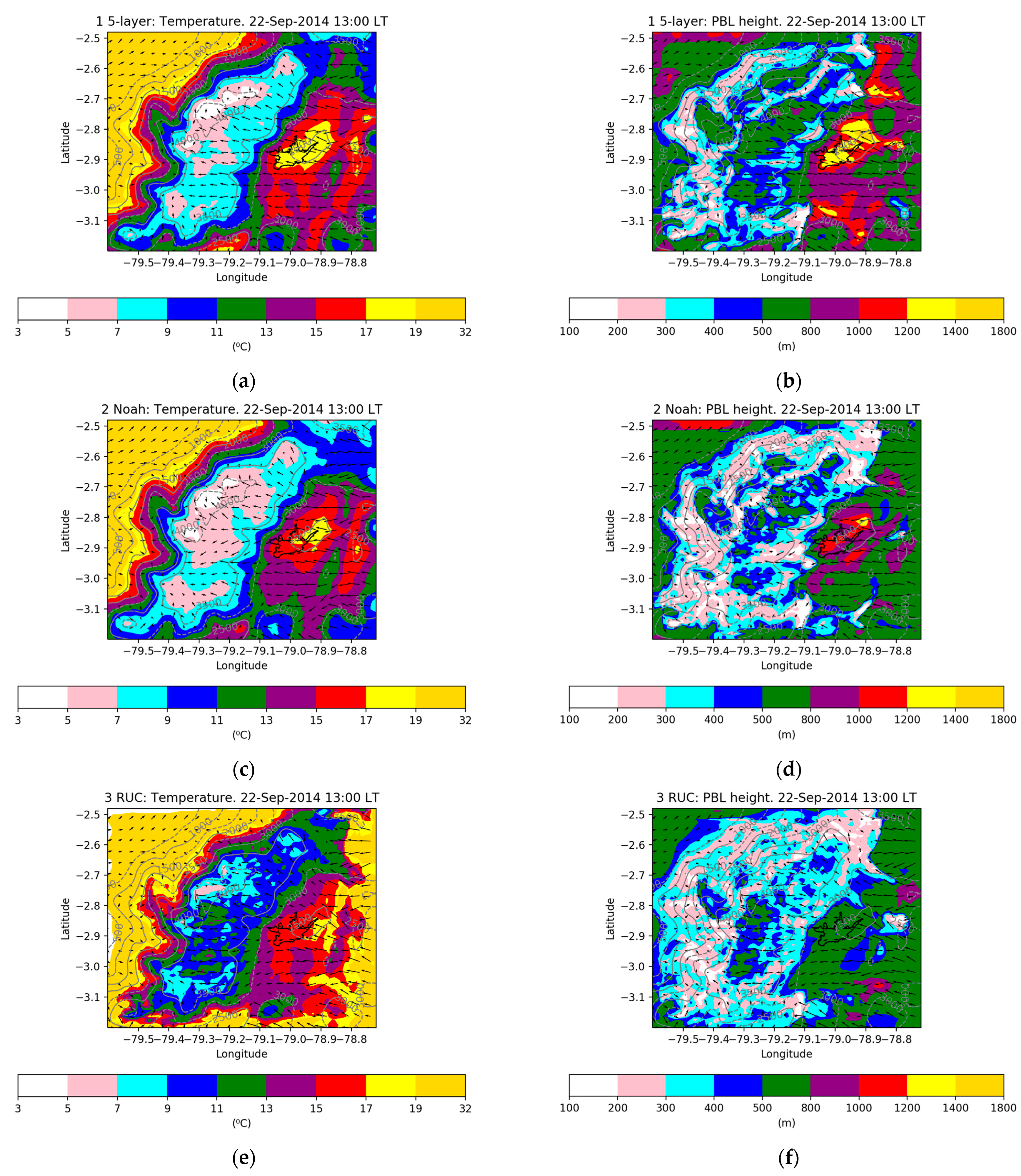
Figure 5 depicts the modeled temperature on 22 September 2014 at 13:00 LT. Over the urban area, the 2 Noah option provided temperatures mostly between 15 and 17 °C. The 1 5-Layer option modeled values mostly between 17 and 19 °C. In the complete urban area, the 3 RUC scheme obtained temperatures ranging from 15 and 17 °C. The 4 Pleim–Xiu option provided values between 13 and 15 °C for the entire urban area. The 5 Noah UCM option provided temperatures consistent with the 2 Noah scheme.
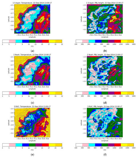
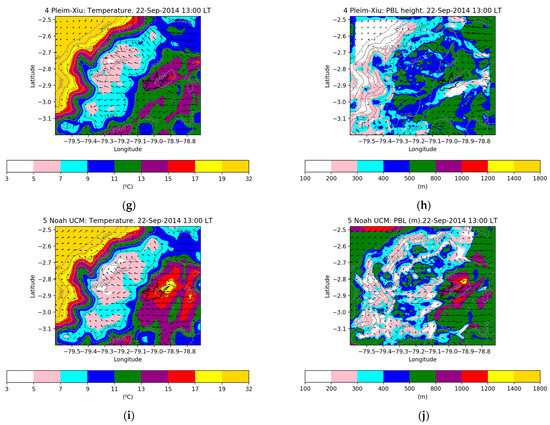
Figure 5.
Modeled temperature and planetary boundary layer height on 22 September 2014 (13:00 LT): (a,b) 1 5-Layer; (c,d) 2 Noah; (e,f) 3 RUC; (g,h) 4 Pleim–Xiu; (i,j) 5 Noah UCM.
Although all the metrics, when using all the options, were in the corresponding benchmark ranges for modeling wind speed, the 2 Noah scheme achieved the best performance (Table 5). Although this scheme, on average, captured the values of the first hours of the day, it overestimated wind speed during the afternoon. This scheme captured the highest percentage (76.9%) of the hourly wind speed records (Table 6). The 4 Pleim–Xiu was the unique scheme that underestimated wind speed between 10:00 to 16:00 LT. The 5 Noah UCM was the option with the highest overestimation (on average, up to 2.2 m s−1 at 15:00 LT) during the afternoon (Figure 3c).
Although the 2 Noah scheme was better in terms of GE (61.9°), none of the options reached values for wind direction that was into the benchmark range (<30°). On average, the wind direction was correctly modeled between 09:00 to 21:00 LT for most of the land surface schemes (Figure 3d). Although found to be the best, the 2 Noah scheme captured only 37.1% of the hourly wind speed records (Table 6).
In all the land surface schemes, the levels of global solar radiation were overestimated (Figure 3b).
We did not find records of Cuenca’s planetary boundary layer height (PBLH). However, for a preliminary comparison, Figure 3e shows five records during the Septembers’ of different years measured in Quito, which is the capital of Ecuador and is an Andean city with similar features to Cuenca in terms of height and topography. Four of these records were taken at the Universidad San Francisco de Quito’s Atmospheric Measurement Station (EMA) at coordinates 0.19° S, 78.4° W, and 2414 masl [42]. The other observation was taken in Izobamba (IZO), which is a station near Quito, at coordinates 0.36° S, 78.55°W, and 3048 masl, and is operated by the National Institute of Meteorology and Hydrology of Ecuador (INAMHI) [43]. In addition, we added the mean PBLH profile of September 2014, deduced from the hourly data of the fifth generation of the European Centre for Medium-Range Weather Forecasts (ECMWF) atmospheric reanalysis dataset (ERA5) [44], specifically for the location of Cuenca.
PBLH observations at 07:00 LT were 218 and 401 m. The closest mean modeled PBLH values were 123 and 79 m, as provided by the 4 Pleim–Xiu and 2 Noah schemes, respectively. At 07:00 LT, the ERA5 dataset indicated 128 m. At 09:00 LT, the observed PBLH (292 m) was near the modeled height (282 m), as per the 2 Noah option. At noon, the observed PBLH (1505 m), was consistent with the results of the 2 Noah (1425 m) and the 1 5-Layer (1622 m) schemes. The PBLH record at 13:00 LT (2025 m) was consistent with the modeled value of the 1 5-Layer (1877 m), and the 2 Noah schemes (1736 m). However, the ERA5 PBLH profile showed values at noon (1245 m) and 13:00 LT (1299 m) that were lower than the records.
3.2. Air Quality
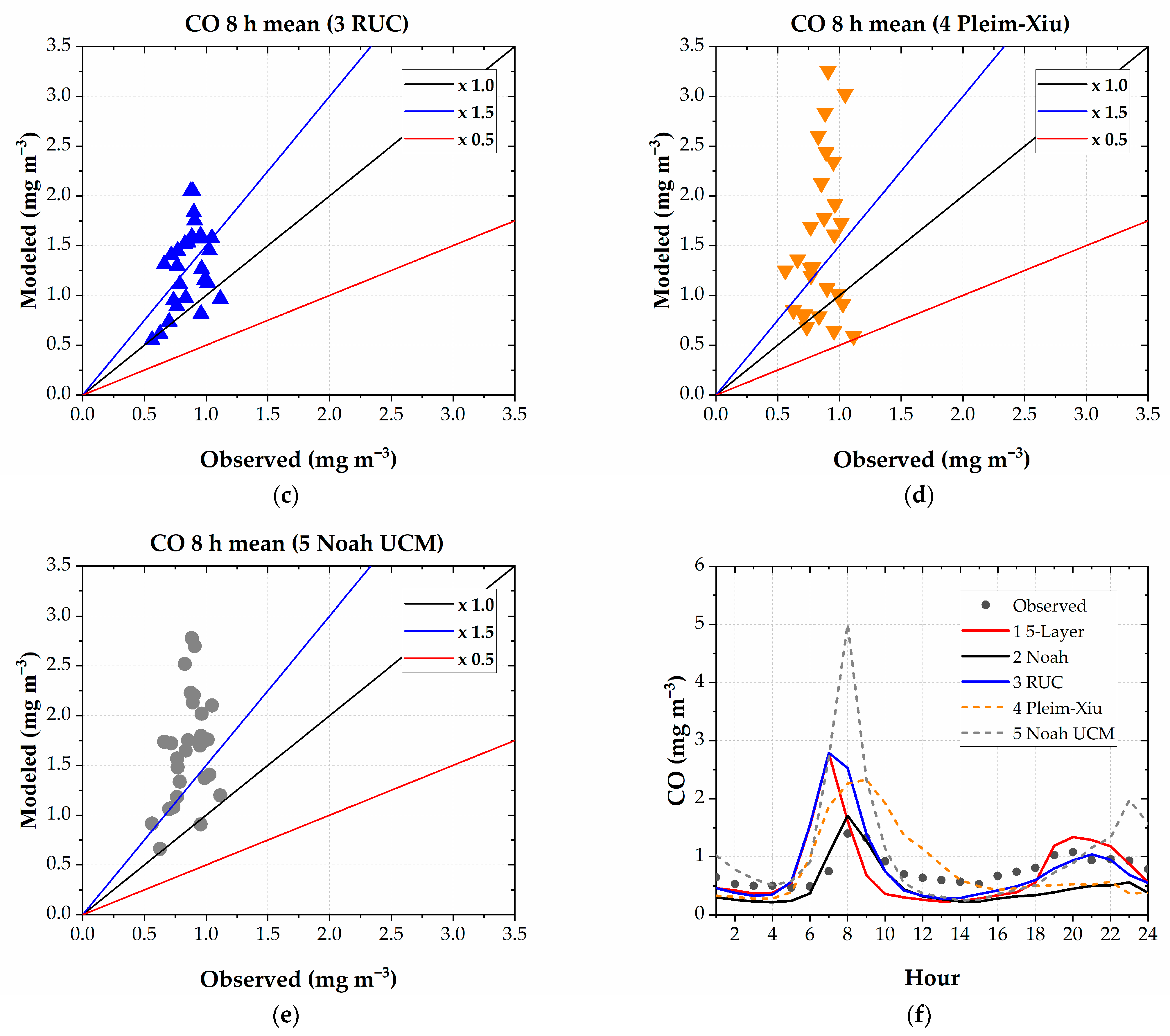
The 2 Noah scheme was best fitted to model the maximum CO daily 1 h mean and the CO daily 8 h mean concentrations (Figure 6b). This scheme also correctly described the mean daily profile during peak CO concentrations (Figure 6f), whereas the other land surface options overestimated the maximum CO levels. On average, the 5 Noah UCM overestimated up to 3.6 mg m−3 of the CO level at 08:00 LT. The 2 Noah scheme received the best metrics for modeling CO concentrations (Table 7). However, this option received no solid linear relationship between the recorded and modeled values (r = 0.41 and r = 0.38, for the maximum CO daily 1 h mean and CO daily 8 h mean, respectively). The 2 Noah option presented the highest percentages of captured records (92.6% for the maximum CO daily 1 h mean, and 100.0% for the maximum CO daily 8 h mean (Table 8). The 5 Noah UCM option showed the lowest performance due to its overestimating the peak CO levels.
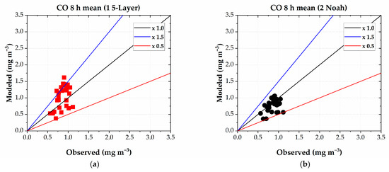
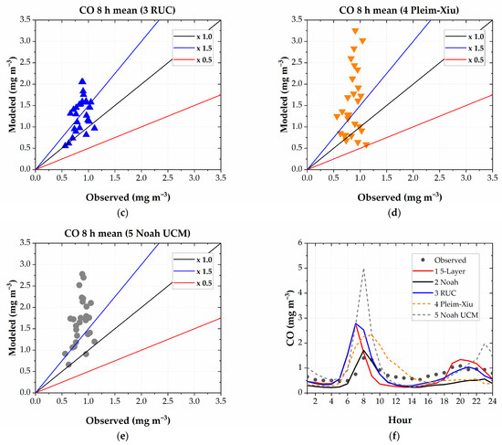
Figure 6.
Observed versus modeled daily CO 8 h maximum mean at the MUN station: (a) 1 5-Layer; (b) 2 Noah; (c) 3 RUC; (d) Pleim–Xiu; (e) 5 Noah UCM. (f) The mean daily profile of hourly CO concentrations.

Table 7.
Metrics for short-term air quality modeling. Bold numbers highlight the schemes with the best performances.

Table 8.
Percentages of the records that were captured by modeling. Air quality variables. Bold numbers highlight the schemes with the best performances.
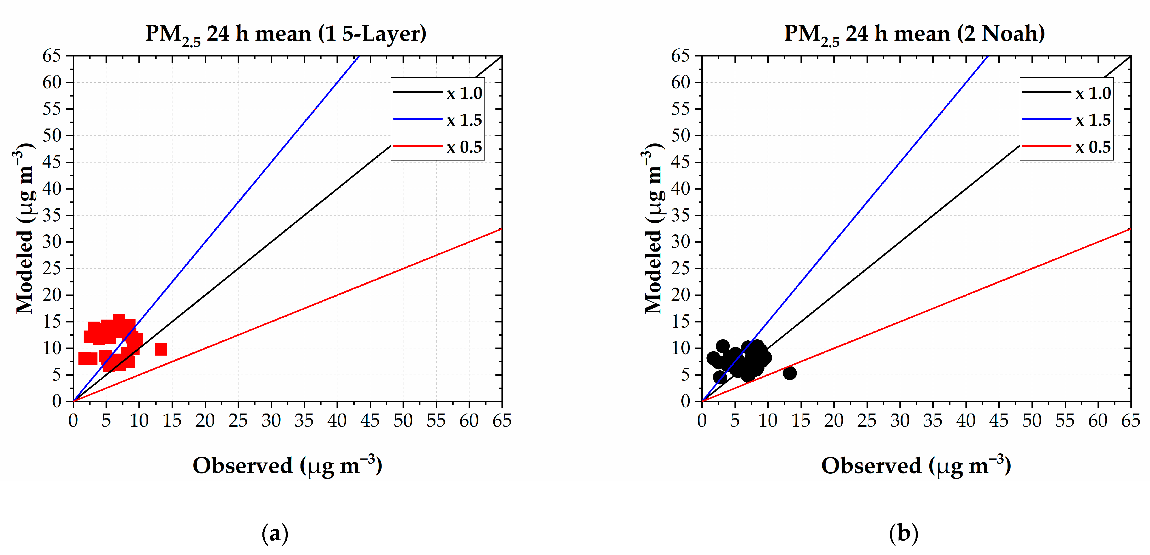
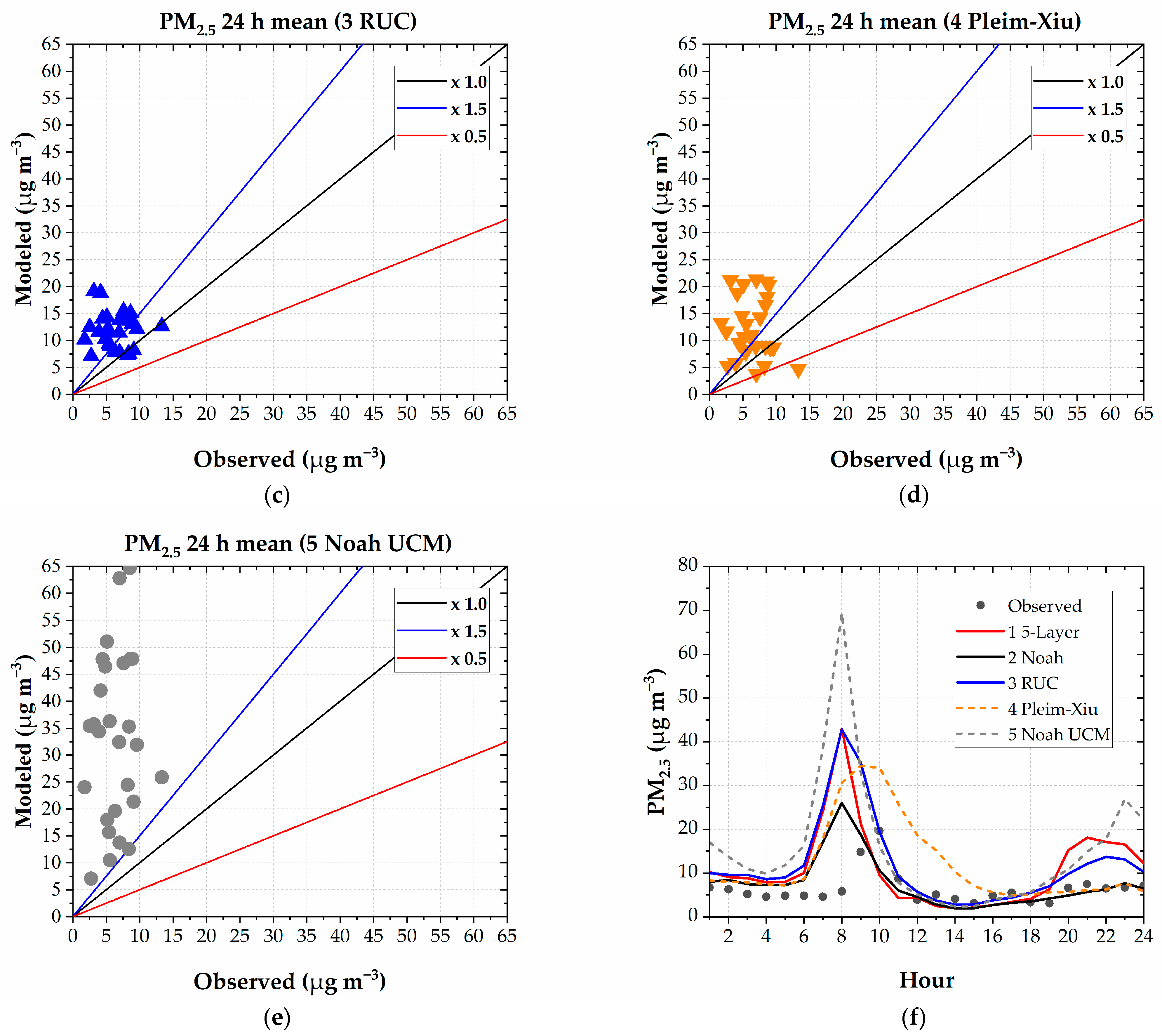
Although somewhat overestimated, the 2 Noah option showed the best performance for modeling the 24 h PM2.5 mean concentrations (Figure 7), which were overestimated by the other options. All the land surface schemes show a weak linear correlation between the recorded and modeled values. The 2 Noah option presented the highest percentages of captured records (63.0%, Table 8). The 5 Noah UCM showed poor performance, whereby it overestimated, to a high degree, the PM2.5 levels (Figure 6e,f) (MB = 26.7 µg m−3).
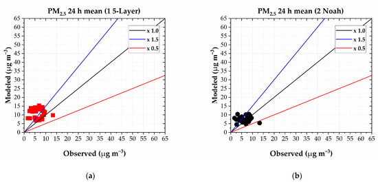
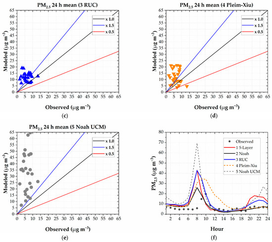
Figure 7.
Observed versus modeled daily PM2.5 24 h mean at the MUN station: (a) 1 5-Layer; (b) 2 Noah; (c) 3 RUC; (d) Pleim–Xiu; (e) 5 Noah UCM. (f) The mean daily profile of hourly PM2.5 concentrations.
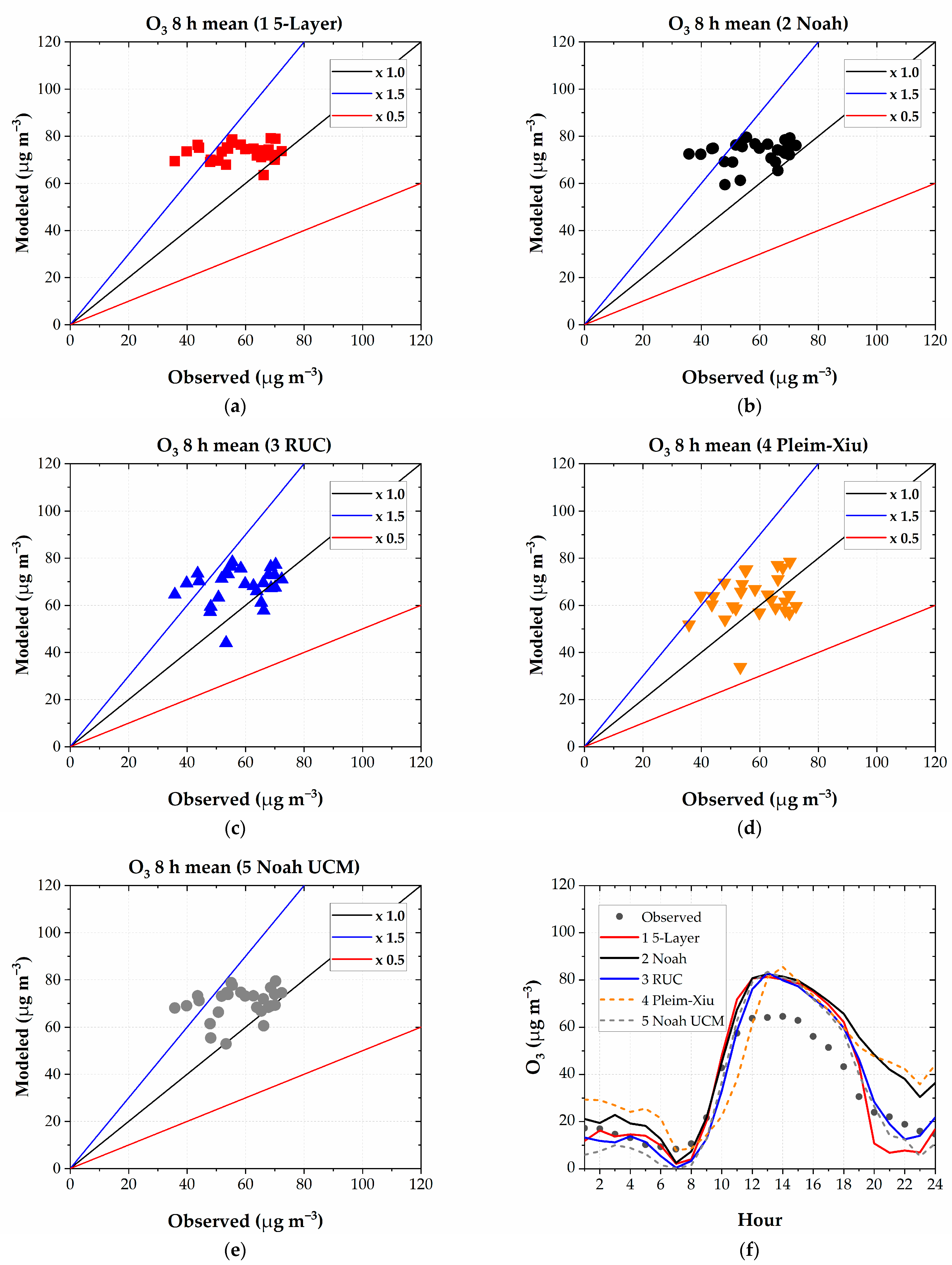
For modeling the maximum 8 h O3 daily mean, the 4 Pleim–Xiu option showed better performance (Table 7, Figure 8). All the schemes delivered no solid linear relationship between the recorded and modeled values (r between 0.09 and 0.25). The 4 Pleim–Xiu option, however, captured 96.3% of records, whereas the other options captured 85.2%.
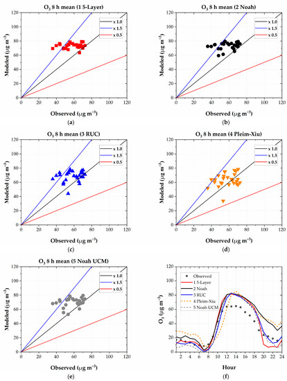
Figure 8.
Observed versus modeled daily O3 8 h maximum mean at the MUN station: (a) 1 5-Layer; (b) 2 Noah; (c) 3 RUC; (d) Pleim–Xiu; (e) 5 Noah UCM. (f) The mean daily profile of hourly O3 concentrations.
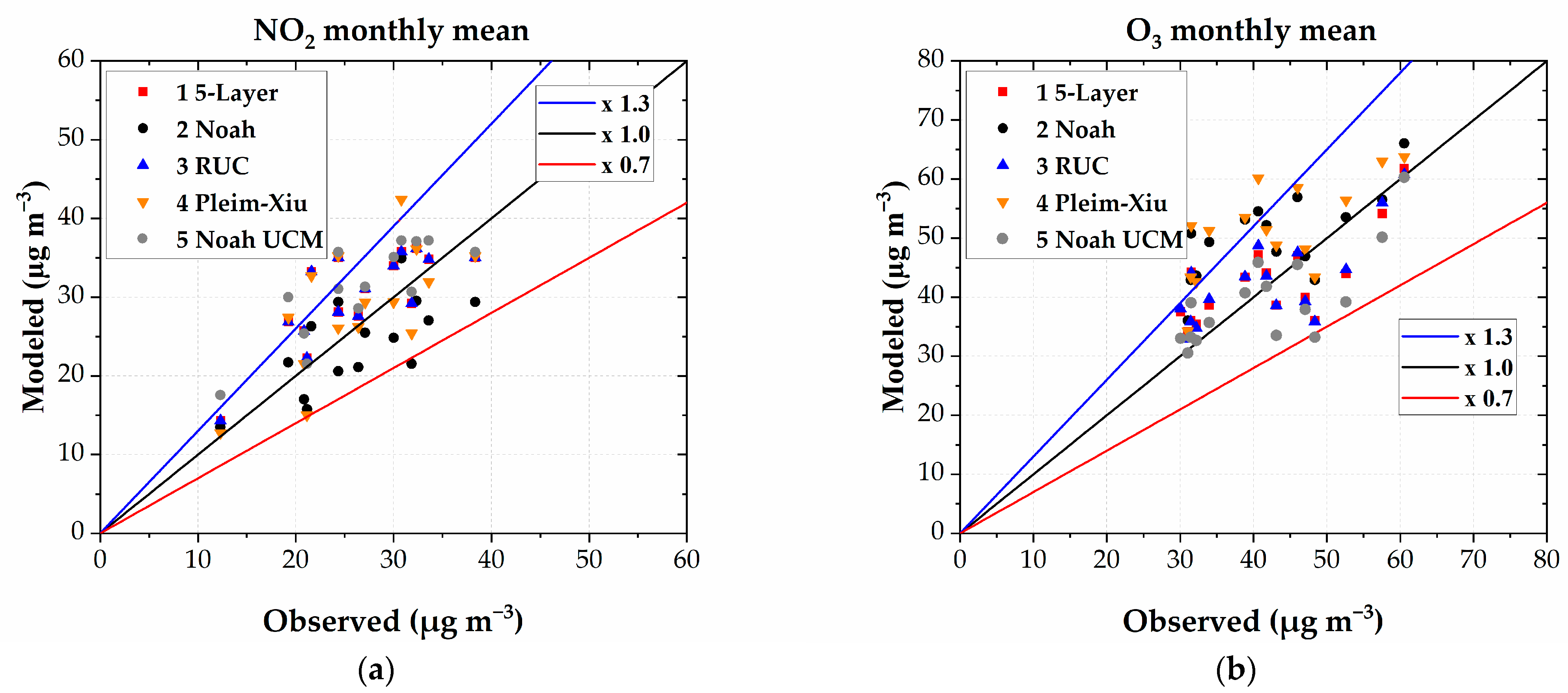
Regarding the NO2 monthly mean concentrations, the 2 Noah scheme captured 93.3% of the records from all passive stations, followed by the 1 5-Layer and 3 RUC options, which captured 80.0% of the records (Table 8, Figure 9a). The 1 5-Layer, 3 RUC, and 5 Noah UCM options adequately modeled 93.8% of the O3 monthly mean concentrations, whereas the 2 Noah and 4 Pleim–Xiu schemes captured 56.3% of the records from the passive stations.
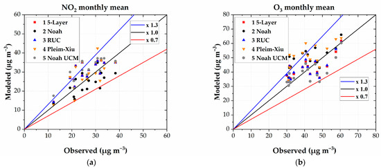
Figure 9.
Passive stations: Observed versus modeled monthly means: (a) NO2 and (b) O3.
4. Discussion and Conclusions
We used a last-generation tool for atmospheric modeling in Cuenca, an Andean city in Southern Ecuador. We assessed the influence of the land surface options from the WRF-Chem V3.2, which is a 3D-Eulerian model used worldwide for the purposes of research and forecasting, to identify the scheme with the best performance for modeling meteorology and air quality. Results indicated that, on average, the 2 Noah scheme was the better option when compared to the 1 5-Layer, 3 RUC, and 4 Pleim–Xiu schemes (which were the other land surface schemes available from the WRF-Chem V3.2). The 2 Noah scheme was the option that best modeled the entire daily mean profile of the surface temperature (Figure 3a), which is a fundamental parameter directly related to the planetary boundary layer height and atmospheric stability. Therefore, this implied that the 2 Noah scheme, with respect to modeling the concentrations of primary and secondary pollutants, was the most successful. The 2 Noah scheme also adequately modeled the daily mean profile of the wind speed from the beginning of the daily cycle up to 13:00 LT (Figure 3c), which was found to be better than the other options. The 4 Pleim–Xiu scheme underestimated the surface temperature and wind speed from 10:00 to 17:00 LT (Figure 3a,c), thus resulting in computing low values regarding the planetary boundary layer height (Figure 3e). Therefore, this increased the computed CO levels, which were higher than the records (Figure 6d,f).
Atmospheric monitoring is scarce in Ecuador, especially for parameters such as the planetary boundary layer height [42,43,45]. We did not find PBLH records from Cuenca. However, five observations of this parameter were measured in Quito, which we preliminary used as a reference. Regarding this, the 2 Noah scheme also provided consistent modeled values of the planetary boundary layer height. In short, more surface and vertical observations will be required in the Andean region of Ecuador for complete assessments of numerical models.
Data from global datasets, such as the ERA5 reanalysis [44], a fifth-generation and one of the most advanced products, need to be assessed for their use in the tropical Andean region of South America [21]. In this sense, Dias-Júnior et al. [46] reported that the data from the ERA5 dataset underestimated the planetary boundary layer height between 15 and 30% when compared to daytime observations in a station downwind from the city of Manaus (Central Amazonia). This underestimation is consistent with the data depicted in Figure 3e, which suggested that the ERA5 data for the location of Cuenca underestimated the PBLH around midday, between 17.3 and 35.9%.
Modeled upward heat fluxes at the surface (Figure 3f) were consistent with the corresponding PBLH profiles. The peak fluxes around midday (between 444 to 566 W m−2) were computed by the 1 5-Layer and 2 Noah, which were the schemes that calculated the highest PBLH values at 14:00 LT (1899–1938 m) (Figure 3e). The 3 RUC and 5 Noah UCM options computed the maximum fluxes of 260 W m−2, with peak PBLH values of 1582 and 1753 m, respectively. The 4 Pleim–Xiu scheme estimated the lowest peak heat flux at the surface (118 W m−2), but at 16:00 LT, rather than at 13:00 or 14:00 LT as the other four schemes had delivered. The Pleim–Xiu option estimated the maximum PBLH in 1209 m, at 17:00 LT. Further, it showed the peaks in temperature and wind speed as displaced to the right when compared to the other schemes. The modeled upward heat fluxes at the surface showed a clear relationship and consistency with the corresponding planetary boundary layer heights.
Our results suggested that the 2 Noah land surface scheme’s better modeling performance would result from its better ability to model the upward heat fluxes at the surface. This preliminary explanation needs to be tested based on observations of heat fluxes and PBLH.
The highest heat fluxes from the 1 5-layer scheme would be related to its approach, which sets the soil moisture with the land use, and the season-dependent constant value without vegetation effects. The other schemes considered the presence of vegetation and delivered more sophisticated treatments for moisture. A detailed analysis of why each option reached its corresponding performance is out of the scope of this study, as this analysis would be challenging due to the complex interactions between the land surface scheme and the other modeling parameterizations.
Our finding is consistent with Rizaa et al. (2018) [4], who reported that the 2 Noah scheme was better than the 3 RUC when modeling (WRF-Chem V3.6.1) the daily mean PM10 levels in Southern Italy, which were produced by a severe dust episode. Our finding is also consistent with the conclusion of Constantinidou et al. (2020) [47], who reported that the 2 Noah scheme was better than the 3 RUC and other schemes for modeling temperature (WRF V3.8.1) in climate simulations in the Middle East-North Africa region. Similarly, Lee et al. [48], especially when modeling the meteorological parameters during a campaign monitoring in South Korea, reported that the 2 Noah scheme produced the best agreement between observations and simulations when compared to the 1 5-Layer, 3 RUC, and 4 Pleim–Xiu schemes.
Our results indicated that modeling meteorological and air quality parameters in Cuenca were sensitive to land surface schemes. Similar conclusions were reported in the literature. Misenis and Zhang (2010) [49] indicated that both meteorological and chemical predictions were sensitive to land surface schemes, when modeling (WRF-Chem V3.6.1) a 5-day summer episode in Houston, United States. Other studies also reported that surface temperature was sensitive to land surface schemes [5,50]. Table 9 compares the main results of this contribution with other assessments on the influence of land surface schemes. Most of the evaluations cover the modeling of meteorological variables.

Table 9.
Comparison with other assessments on the influence of land surface schemes.
Contrary to the finding of this study, other studies have reported that other land surface schemes were better than the 2 Noah scheme. Lu et al. (2021) [53] indicated the community land surface scheme was better than the 3 RUC scheme and an improved version of the 2 Noah scheme when modeling temperature and rainfall (WRF V4.0) during summer in Central Asia. The 1 5-Layer scheme, has been reported as the simplest land surface scheme in terms of structure and physics and was found to be better than an improved version of the 2 Noah scheme for modeling (WRF V4.0) meteorological variables over the south of Chile [3]. The 4 Pleim–Xiu was better than the 2 Noah scheme for modeling sensible heat fluxes (WRF V3.7.1) in Oregon, United States [2]. However, 2 Noah’s improved version provided better results than the 4 Pleim–Xiu scheme, specifically when the North American Regional Reanalysis forcing dataset was used.
Combining the 2 Noah scheme and the urban canopy model option did not show benefits in Cuenca when compared to results with the Noah scheme alone. Moreover, this combination produced the poorest computed results due to overestimating CO and PM2.5 levels. These results are partly explained by the underestimation of surface temperature at hours of peak emissions of the primary pollutants, which were accompanied by lower planetary boundary layer heights (Figure 3e) when compared to the 2 Noah option, thereby limiting the volume of the atmosphere with respect to dispersing primary pollutants. The results suggested that, although the urban canopy model can consider the urban effects at the subgrid-scale, this feature does not necessarily improve the modeling performance. The decrease in performance when modeling with the 2 Noah scheme and the urban canopy model is consistent with the conclusion by Liao et al. (2014) [55], who reported that when using the urban canopy model, higher PM10 concentrations were computed (WRF-Chem V3.2.1), specifically when modeling climate and air quality in the Yangtze River Delta, China. Although the urban canopy models describe the effects of urban areas at a subgrid-scale (less than 1 km for the inner domain of Cuenca), it seems that this option from WRF-Chem V3.2 is unsuitable or has properties that do not represent the urban area of Cuenca. Due to its nature, urban canopy models are expected to improve the modeling performance.
Interestingly all the options, including the 5 Noah UCM, showed good performances for modeling O3 concentrations, capturing between 85.2 and 96.3% of the maximum O3 8 h mean daily records (Table 8). Except for the 4 Pleim–Xiu scheme, the other options tend to overestimate O3 levels (Figure 8). The presence of the WE in the historic center of Cuenca indicates that around the MUN station, the O3 abundance is promoted by decreasing NOx emissions and that an increase of NOx will thus reduce the O3 levels. On the other hand, an increase or decrease in NMVOC emissions will increase or decrease the production of O3, respectively. This feature needs to be considered for the new emissions inventory for Cuenca, where the ratio between NMVOC to NOx should be compatible with a regime for O3 production that is limited by NMVOC emissions.
Our results and conclusions from other studies suggest that dedicated assessments should be conducted to identify an appropriate land surface option for each study region.
Our results suggest that for the purposes of modeling meteorology and air quality with the WRF-Chem V3.2 in the Andean region of Ecuador, the 2 Noah scheme would provide properly computed values of surface temperature, wind speed, and air quality variables. Therefore, we suggest that the 2 Noah land surface scheme be utilized for assessing the quality of Cuenca’s new atmospheric emission inventory, which is currently in preparation.
Based on this and previous contributions, we preliminary recommend the following options for modeling with the WRF-Chem V3.2, both for modeling the meteorology and air quality in the Andean region of Ecuador:
- Land use categories: Based on the USGS dataset and categories (as per this contribution);
- Global atmospheric dataset: FNL [21];
- Land surface scheme: Noah (as per this contribution);
- Urban Canopy Model: None (as per this contribution);
- Planetary Boundary Layer: Yonsei University option [20];
- Chemical mechanisms and aerosol modules: CBMZ and MOSAIC with direct effects [20,23].
Our contribution provided insights for atmospheric studies in the Andean region of Ecuador, which is a complex area in which atmospheric modeling is challenging. This is due to the influence of the Andes chain, the intertropical converge zone, and the poor coverage of atmospheric monitoring, both at the surface and especially in terms of vertical sounding [21,44]. Our findings help to understand the influence of land surface schemes in modeling meteorology and air quality, which are valuable features because, in most of the studies, we found that only meteorological variables were assessed.
In the future, other options need to be explored, such as using an updated version of WRF-Chem, as well as determining the corresponding versions of the land surface and urban canopy model options. In addition, although the land uses a map of this assessment that acceptably described the current situation in Cuenca, it can be updated. For this purpose, it is necessary to update the data in the USGS or to assess the data coming from the Moderate Resolution Imaging Spectroradiometer (MODIS), or even from dedicated local studies in Cuenca to describe in the best way the land uses categories and their properties.
Although temperature and wind speed were adequately modeled in Cuenca, other meteorological variables, such as solar radiation and wind direction, require improved modeling performance. For solar radiation, dedicated studies for assessing the cumulus, land surface, and microphysics options can be evaluated. One limitation of modeling in the Andean region is the lack of dedicated schemes. We have used options developed and tested mainly in the Northern Hemisphere. Therefore, the development or updating of the parameterization options is strongly desirable, specifically by considering the features of the Andean region. Moreover, updated topography can improve the modeling performance for wind direction. Additionally, the potential benefits from data assimilation need to be evaluated.
Funding
This research was funded by the USFQ Poli-Grants 2022–2023 program.
Informed Consent Statement
Not applicable.
Data Availability Statement
Not applicable.
Acknowledgments
This research is part of the “Emisiones atmosféricas y Calidad del Aire en el Ecuador 2022–2023” project. Simulations were done at the High-Performance Computing system at the Universidad San Francisco de Quito. Publication of this article was funded by the Universidad San Francisco de Quito USFQ Research Publication Fund.
Conflicts of Interest
The author declares no conflict of interest.
References
- Warner, T.T. Numerical Weather and Climate Prediction; Cambridge University Press: Cambridge, UK, 2011. [Google Scholar]
- Sun, X.; Holmes, H.; Osibanjo, O.; Sun, Y.; Ivey, C. Evaluation of Surface Fluxes in the WRF Model: Case Study for Farmland in Rolling Terrain. Atmosphere 2017, 8, 197. [Google Scholar] [CrossRef]
- Somos-Valenzuela, M.; Manquehual-Cheuque, F. Evaluating Multiple WRF Configurations and Forcing over the Northern Patagonian Icecap(NPI) and Baker River Basin. Atmosphere 2020, 11, 815. [Google Scholar] [CrossRef]
- Rizza, U.; Miglietta, M.M.; Mangia, C.; Ielpo, P.; Morichetti, M.; Iachini, C.; Virgili, S.; Passerini, G. Sensitivity of WRF-Chem Model to Land Surface Schemes: Assessment in a Severe Dust Outbreak Episode in the Central Mediterranean(Apulia Region). Atmos. Res. 2018, 201, 168–180. [Google Scholar] [CrossRef]
- Liu, L.; Ma, Y.; Menenti, M.; Zhang, X.; Ma, W. Evaluation of WRF Modeling in Relation to Different Land Surface Schemes and Initial and Boundary Conditions: A Snow Event Simulation Over the Tibetan Plateau. J. Geophys. Res. Atmos. 2019, 124, 209–226. [Google Scholar] [CrossRef]
- Stensrud, D. Parameterization Schemes: Keys to Understanding Numerical Weather Prediction Models; Cambridge University Press: New York, NY, USA, 2009. [Google Scholar]
- Fisher, R.A.; Koven, C.D. Perspectives on the Future of Land Surface Models and the Challenges of Representing Complex Terrestrial Systems. J. Adv. Model. Earth Syst. 2020, 12, e2018MS001453. [Google Scholar] [CrossRef]
- Zeng, X.-M.; Wang, N.; Wang, Y.; Zheng, Y.; Zhou, Z.; Wang, G.; Chen, C.; Liu, H. WRF-Simulated Sensitivity to Land Surface Schemes in Short and Medium Ranges for a High-Temperature Event in East China: A Comparative Study: WRF Sensitivity to Land Surface Schemes. J. Adv. Model. Earth Syst. 2015, 7, 1305–1325. [Google Scholar] [CrossRef]
- Skamarock, W.C.; Klemp, J.B.; Dudhia, J.; Gill, D.O.; Barker, D.M.; Duda, M.G.; Huang, X.-Y.; Wang, W.; Powers, J.G. A Description of the Advanced Research WRF Version 3. 2008. Available online: https://opensky.ucar.edu/islandora/object/technotes:500 (accessed on 12 February 2023).
- Dudhia, J. A multi-layer soil temperature model for MM5. Workshop Boulder. In Proceedings of the Sixth Annual PSU/NCAR Mesoscale Model Users’ Workshop, Bouilder, CO, USA, 22–24 July 1996; pp. 49–50. [Google Scholar]
- Chen, F.; Dudhia, J. Coupling an Advanced Land Surface—Hydrology Model with the Penn State–NCAR MM5 Modeling System. Part II: Preliminary Model Validation. Mon. Weather Rev. 2001, 129, 587–604. [Google Scholar] [CrossRef]
- Smirnova, T.G.; Brown, J.M.; Benjamin, S.G. Performance of Different Soil Model Configurations in Simulating Ground Surface Temperature and Surface Fluxes. Mon. Weather Rev. 1997, 125, 1870–1884. [Google Scholar] [CrossRef]
- Smirnova, T.G.; Brown, J.M.; Benjamin, S.G.; Kim, D. Parameterization of Cold-Season Processes in the MAPS Land-Surface Scheme. J. Geophys. Res. Atmos. 2000, 105, 4077–4086. [Google Scholar] [CrossRef]
- Pleim, J.E.; Xiu, A. Development and Testing of a Surface Flux and Planetary Boundary Layer Model for Application in Mesoscale Models. J. Appl. Meteorol. 1995, 34, 16–32. [Google Scholar] [CrossRef]
- Xiu, A.; Pleim, J.E. Development of a Land Surface Model. Part I: Application in a Mesoscale Meteorological Model. J. Appl. Meteorol. 2001, 40, 192–209. [Google Scholar] [CrossRef]
- Espinoza Claudia, C. Informe de Calidad Del Aire Cuenca 2021; EMOV EP: Cuenca, Ecuador, 2022; Available online: https://www.researchgate.net/publication/362194795_Informe_de_Calidad_del_Aire_Cuenca_2021 (accessed on 12 February 2023).
- World Health Organization. WHO Global Air Quality Guidelines: Particulate Matter(PM2.5 and PM10), Ozone, Nitrogen Dioxide, Sulfur Dioxide and Carbon Monoxide; World Health Organization: Geneva, Switzerland, 2021.
- World Health Organization (Ed.) Air Quality Guidelines: Global Update 2005: Particulate Matter, Ozone, Nitrogen Dioxide, and Sulfur Dioxide; World Health Organization: Copenhagen, Denmark, 2006.
- Parra, R.; Cadena, E.; Flores, C. Maximum UV Index Records(2010–2014) in Quito(Ecuador) and Its Trend Inferred from Remote Sensing Data (1979–2018). Atmosphere 2019, 10, 787. [Google Scholar] [CrossRef]
- Parra, R. Performance Studies of Planetary Boundary Layer Schemes in WRF-Chem for the Andean Region of Southern Ecuador. Atmos. Pollut. Res. 2018, 9, 411–428. [Google Scholar] [CrossRef]
- Parra, R. Effect of Global Atmospheric Datasets in Modeling Meteorology and Air Quality in the Andean Region of Ecuador. Aerosol Air Qual. Res. 2022, 22, 210292. [Google Scholar] [CrossRef]
- Parra, R. Effects of Aerosols Feedbacks in Modeling Meteorology and Air Quality in the Andean Region of Southern Ecuador; WIT Press: Santiago de Compostela, Spain, 2021; pp. 39–50. [Google Scholar] [CrossRef]
- Parra, R.; Espinoza, C. Insights for Air Quality Management from Modeling and Record Studies in Cuenca, Ecuador. Atmosphere 2020, 11, 998. [Google Scholar] [CrossRef]
- Parra, R.; Saud, C.; Espinoza, C. Simulating PM2.5 Concentrations during New Year in Cuenca, Ecuador: Effects of Advancing the Time of Burning Activities. Toxics 2022, 10, 264. [Google Scholar] [CrossRef]
- EMOV-EP. Inventario de Emisiones Atmosféricas Del Cantón Cuenca 2014. 2016. [CrossRef]
- WRF Model Users Site. Available online: https://www2.mmm.ucar.edu/wrf/users/ (accessed on 30 December 2022).
- CISL RDA: NCEP FNL Operational Model Global Tropospheric Analyses, Continuing from July 1999. Available online: https://rda.ucar.edu/datasets/ds083.2/ (accessed on 30 December 2022).
- Zaveri, R.A.; Peters, L.K. A New Lumped Structure Photochemical Mechanism for Large-Scale Applications. J. Geophys. Res. Atmospheres 1999, 104, 30387–30415. [Google Scholar] [CrossRef]
- Zaveri, R.A.; Easter, R.C.; Fast, J.D.; Peters, L.K. Model for Simulating Aerosol Interactions and Chemistry(MOSAIC). J. Geophys. Res. 2008, 113, D13204. [Google Scholar] [CrossRef]
- Hong, S.-Y.; Dudhia, J.; Chen, S.-H. A Revised Approach to Ice Microphysical Processes for the Bulk Parameterization of Clouds and Precipitation. Mon. Weather Rev. 2004, 132, 103–120. [Google Scholar] [CrossRef]
- Mlawer, E.J.; Taubman, S.J.; Brown, P.D.; Iacono, M.J.; Clough, S.A. Radiative Transfer for Inhomogeneous Atmospheres: RRTM, a Validated Correlated-k Model for the Longwave. J. Geophys. Res. Atmos. 1997, 102, 16663–16682. [Google Scholar] [CrossRef]
- Chou, M.-D.; Suarez, M.J. A Solar Radiation Parameterization for Atmospheric Studies; NASA/TM-1999-104606/VOL15; NASA: Washington, DC, USA, 1999. Available online: https://ntrs.nasa.gov/citations/19990060930 (accessed on 30 December 2022).
- Paulson, C.A. The Mathematical Representation of Wind Speed and Temperature Profiles in the Unstable Atmospheric Surface Layer. J. Appl. Meteorol. 1970, 9, 857–861. [Google Scholar] [CrossRef]
- Hong, S.-Y.; Noh, Y.; Dudhia, J. A New Vertical Diffusion Package with an Explicit Treatment of Entrainment Processes. Mon. Weather Rev. 2006, 134, 2318–2341. [Google Scholar] [CrossRef]
- Grell, G.A. Prognostic Evaluation of Assumptions Used by Cumulus Parameterizations. Mon. Weather Rev. 1993, 121, 764–787. [Google Scholar] [CrossRef]
- Kusaka, H.; Kondo, H.; Kikegawa, Y.; Kimura, F. A Simple Single-Layer Urban Canopy Model For Atmospheric Models: Comparison With Multi-Layer And Slab Models. Bound. Layer Meteorol. 2001, 101, 329–358. [Google Scholar] [CrossRef]
- Kusaka, H.; Kimura, F. Coupling a Single-Layer Urban Canopy Model with a Simple Atmospheric Model: Impact on Urban Heat Island Simulation for an Idealized Case. J. Meteorol. Soc. Jpn. Ser. II 2004, 82, 67–80. [Google Scholar] [CrossRef]
- Chen, F.; Tewari, M.; Kusaka, H.; Warner, T. Current Status of Urban Modeling in the Community Weather Research and Forecast (WRF) Model (2006—Annual2006_6urban). Available online: https://ams.confex.com/ams/Annual2006/techprogram/paper_98678.htm (accessed on 30 December 2022).
- The Application of Models under the European Union’s Air Quality Directive: A Technical Reference Guide—European Environment Agency. Available online: https://www.eea.europa.eu/publications/fairmode (accessed on 30 December 2022).
- Simon, H.; Baker, K.R.; Phillips, S. Compilation and Interpretation of Photochemical Model Performance Statistics Published between 2006 and 2012. Atmos. Environ. 2012, 61, 124–139. [Google Scholar] [CrossRef]
- World Health Organization, Regional Office for Europe. Air Quality Guidelines for Europe; World Health Organization, Regional Office for Europe: Geneva, Switzerland, 2000.
- Cazorla, M.; Juncosa, J. Planetary Boundary Layer Evolution over an Equatorial Andean Valley: A Simplified Model Based on Balloon-Borne and Surface Measurements. Atmos. Sci. Lett. 2018, 19, e829. [Google Scholar] [CrossRef]
- Muñoz, L.E.; Campozano, L.V.; Guevara, D.C.; Parra, R.; Tonato, D.; Suntaxi, A.; Maisincho, L.; Páez, C.; Villacís, M.; Córdova, J.; et al. Comparison of Radiosonde Measurements of Meteorological Variables with Drone, Satellite Products, and WRF Simulations in the Tropical Andes: The Case of Quito, Ecuador. Atmosphere 2023, 14, 264. [Google Scholar] [CrossRef]
- ERA5 Hourly Data on Pressure Levels from 1959 to Present. Available online: https://cds.climate.copernicus.eu/cdsapp#!/dataset/reanalysis-era5-pressure-levels?tab=form (accessed on 12 February 2023).
- Cazorla, M.; Parra, R.; Herrera, E.; da Silva, F.R. Characterizing Ozone throughout the Atmospheric Column over the Tropical Andes from in Situ and Remote Sensing Observations. Elem. Sci. Anthr. 2021, 9, 00019. [Google Scholar] [CrossRef]
- Dias-Júnior, C.Q.; Carneiro, R.G.; Fisch, G.; D’Oliveira, F.A.F.; Sörgel, M.; Botía, S.; Machado, L.A.T.; Wolff, S.; dos Santos, R.M.N.; Pöhlker, C. Intercomparison of Planetary Boundary Layer Heights Using Remote Sensing Retrievals and ERA5 Reanalysis over Central Amazonia. Remote Sens. 2022, 14, 4561. [Google Scholar] [CrossRef]
- Constantinidou, K.; Hadjinicolaou, P.; Zittis, G.; Lelieveld, J. Performance of Land Surface Schemes in the WRF Model for Climate Simulations over the MENA-CORDEX Domain. Earth Syst. Environ. 2020, 4, 647–665. [Google Scholar] [CrossRef]
- Lee, C.B.; Kim, J.-C.; Belorid, M.; Zhao, P. Performance Evaluation of Four Different Land Surface Models in WRF. Asian J. Atmos. Environ. 2016, 10, 42–50. [Google Scholar] [CrossRef]
- Misenis, C.; Zhang, Y. An Examination of Sensitivity of WRF/Chem Predictions to Physical Parameterizations, Horizontal Grid Spacing, and Nesting Options. Atmos. Res. 2010, 97, 315–334. [Google Scholar] [CrossRef]
- Teklay, A.; Dile, Y.T.; Asfaw, D.H.; Bayabil, H.K.; Sisay, K. Impacts of Land Surface Model and Land Use Data on WRF Model Simulations of Rainfall and Temperature over Lake Tana Basin, Ethiopia. Heliyon 2019, 5, e02469. [Google Scholar] [CrossRef]
- Zhuo, L.; Dai, Q.; Han, D.; Chen, N.; Zhao, B. Assessment of Simulated Soil Moisture from WRF Noah, Noah-MP, and CLM Land Surface Schemes for Landslide Hazard Application. Hydrol. Earth Syst. Sci. 2019, 23, 4199–4218. [Google Scholar] [CrossRef]
- Tomasi, E.; Giovannini, L.; Zardi, D.; de Franceschi, M. Optimization of Noah and Noah_MP WRF Land Surface Schemes in Snow-Melting Conditions over Complex Terrain. Mon. Weather Rev. 2017, 145, 4727–4745. [Google Scholar] [CrossRef]
- Lu, S.; Guo, W.; Xue, Y.; Huang, F.; Ge, J. Simulation of Summer Climate over Central Asia Shows High Sensitivity to Different Land Surface Schemes in WRF. Clim. Dyn. 2021, 57, 2249–2268. [Google Scholar] [CrossRef]
- Jin, J.; Miller, N.L.; Schlegel, N. Sensitivity Study of Four Land Surface Schemes in the WRF Model. Adv. Meteorol. 2010, 2010, 1–11. [Google Scholar] [CrossRef]
- Liao, J.; Wang, T.; Wang, X.; Xie, M.; Jiang, Z.; Huang, X.; Zhu, J. Impacts of Different Urban Canopy Schemes in WRF/Chem on Regional Climate and Air Quality in Yangtze River Delta, China. Atmos. Res. 2014, 145–146, 226–243. [Google Scholar] [CrossRef]
Disclaimer/Publisher’s Note: The statements, opinions and data contained in all publications are solely those of the individual author(s) and contributor(s) and not of MDPI and/or the editor(s). MDPI and/or the editor(s) disclaim responsibility for any injury to people or property resulting from any ideas, methods, instructions or products referred to in the content. |
© 2023 by the author. Licensee MDPI, Basel, Switzerland. This article is an open access article distributed under the terms and conditions of the Creative Commons Attribution (CC BY) license (https://creativecommons.org/licenses/by/4.0/).


