Influence of Meteorological Parameters on the Urban Heat Island in Moscow

Abstract

The urban heat island (UHI) intensity in Moscow and the influence of various meteorological parameters are discussed using weather station data. The maximal and average in-space UHI intensities, i.e., a comparison of air temperature T either in the city centre or in the whole urban area together with rural zone have averaged 1.9 and 0.9 °C, respectively, in recent years. The UHI in Moscow has stabilized over the past decade and is not growing. Under conditions of a strong anticyclone, the maximal UHI intensity in space and time reaches 11–12 °C. Low cloudiness and amplitudes of diurnal air temperature, as well as surface temperature, demonstrate the closest relationship with the UHI intensity among other parameters with the correlation coefficient of up to −0.67 for low cloudiness and the maximal UHI intensity. The effect of wind speed, total cloudiness and relative humidity on the UHI is slightly weaker, but still significant. The relationships of all meteorological parameters with the maximal UHI intensity are closer than those with the average one. The multiple correlation coefficient between the maximal UHI intensity and both parameters (low cloudiness and average daily wind speed) is 0.76–0.82. The UHI intensity function of air temperature has a minimum in the range from −4 to 0 °C; its growth both at lower and higher T is due to the influence of anticyclonic weather. The UHI intensity function of wind speed decreases with wind strength. The threshold value at which this function asymptotically approaches its lower limit is 10 m/s in the 40–200 m air layer. The UHI intensity functions of both total and low cloudiness decrease with increasing cloudiness and the differences between them are significant if the cloud cover is more than 50%.

1. Introduction

The urban heat island (UHI) is well-known phenomenon that has been studied in almost all big and many medium-sized cities of the world; a lot of papers about it were collected by Kratzer, Landsberg, Oke et al. [1,2,3]. Studying the UHI is important, as it affects health and thermal comfort of the urban population. This creates an additional heat stress during extreme heat waves, but, on the other hand, reduces the damage to human health from severe frosts. This phenomenon increases energy costs for air conditioning in summer but results in savings on heating in winter. In addition, higher air temperature in cities affects the development of vegetation, lengthening the growing season in mid-latitudes.

The UHI in Moscow has been studied in many papers, initially by Bogolepow [4]. Various studies of this phenomenon, containing the results of both measurements and modeling are collected in [5]. The annual course of the UHI in Moscow was studied in Rubinshtein and Ginzburg and Lokoshchenko and Alekseeva [6,7]; long-term changes in this phenomenon were discussed in Lokoshchenko [8]; the vertical structure of the UHI over Moscow was studied both from remote sensing data in Kadygrov et al. [9] and measurements in Lokoshchenko et al. [10]. However, the influence of meteorological parameters on the UHI in Moscow has never been studied as separate task. In addition, the UHI intensity functions of meteorological parameters in Moscow conditions have also never before been created and analyzed. Thus, this paper fills this research gap.

Usually, the main UHI parameter, the so-called UHI intensity, i.e., the difference between the air temperature T inside and outside the city, the UHI spatial structure, urban heat balance including anthropogenic heat flux, modeling of street canyons, and some other aspects of urban climatology are discussed in the literature. However, studies of the influence of meteorological parameters on the UHI intensity are still insufficient. Sometimes authors consider an axiom the strongest influence of two factors, lower cloudiness and wind speed, without their comparative testing. For example, Elemér et al. [11] studied long-term changes in the three the main parameters favorable for the UHI generation (low cloudiness, low wind speed and no precipitation) in Debrecen, Hungary, over the period from 1961 to 2009. Thus, they investigated the dynamics of natural factors that create the UHI but did not check whether these factors are indeed the main ones. This conclusion, i.e., that the strongest influence on the UHI intensity is exerted by cloudiness and wind speed, was obtained for this city in Kratzer [1] and for another Hungarian city, Szeged, in Unger [12]. In addition, Unger presented empirical functions of the UHI intensity of both the wind speed and cloudiness. The same functions were also demonstrated for the UHI of Melbourne, Australia, by Morris et al. [13]. Long-term changes in the mean annual values of the five parameters affecting the UHI (wind speed, total and low cloudiness, atmospheric pressure, relative humidity and precipitation), as well as changes in the UHI intensity, were demonstrated over the period from 1979 to 2013 in Shanghai, China, in Qunfang Huang et al. [14]. In addition, the authors calculated the UHI intensity empirical functions of wind speed, total cloudiness, relative humidity, and combined functions of two different parameters. Baomin Wang et al. [15] analyzed the effect of four meteorological values (cloud cover, wind speed, relative humidity and daily precipitation) on the intensity of urban heat islands over the Pearl River Delta, Southern China. As a result, they determined that low cloud cover demonstrates the strongest relationship (the largest absolute values of the correlation coefficient) with the UHI value, among other parameters, of up to −0.56. In contrast, in Ibadan, Nigeria, a similar analysis demonstrated little effect of cloud cover on the UHI intensity, but a significant effect of two other parameters, wind speed and relative humidity in Anibaba et al. [16]. It may be that the weak influence of cloud cover is due to climatic features: cloudiness in Nigeria during almost the entire year, except for December and January, is extremely low. A similar comparative analysis of the influence of various parameters on the UHI intensity in Vienna, Austria, was carried out by Böhm and Gabl [17] using not only simple correlation coefficients, but also multiple correlations between the UHI intensity and combined cloudiness and wind speed. Several estimates of the night-time UHI intensity depending on various cloudiness and wind speed were presented for Salamanca, Spain, by Alonso et al. [18].

Unlike other authors, Baomin Wang et al. [15] calculated a slightly different parameter instead of the traditional UHI intensity: the frequency of the UHI at its intensity of >0.5 °C. For this frequency, they obtained empirical functions of four meteorological parameters: cloudiness, wind speed, relative humidity and precipitation intensity. A clear difference in the UHI intensity between low values on days with precipitation and high values on days without precipitation was confirmed in Seoul, Southern Korea, by Sang-Hyun Lee and Jong-Jin Baik [19]. The close relation between the UHI intensity and synoptic processes leading to anticyclonic weather is well known; this was confirmed by synoptic analysis in Unger, Alonso et al., Sang-Hyun Lee and Jong-Jin Baik [12,18,19]. Globally generalized relations between the surface urban heat island (SUHI) intensity and both air temperature T and precipitation in the biggest cities depending on the season and time of day according to satellite data are presented in Long Li et al. [20]. According to these results, in most European cities, the correlation is significantly negative at any time of the day in winter, while in summer its sign is different: the correlation is significantly negative during the day but becomes significantly positive at night.

The main goal of the authors was to study and compare the influence of various meteorological parameters on the UHI of Moscow and, as a result, to determine some parameter that generates this phenomenon to the greatest extent. Empirical dependences of the UHI intensity on meteorological parameters for Moscow are calculated and compared with similar ones in other cities. In addition, the spatial structure of the UHI in Moscow is considered in detail.

2. Materials and Methods

2.1. Study Area

We consider Moscow in its traditional borders in the shape of a turtle until 2012, when the expansion of the urban area was announced. However, the so-called “New Moscow” still remains a rural area with low a population density. The population of Moscow in its old borders is 12.2 million people; the area is 1081 km². Thus, the population density in “Old Moscow” is approximately 11,280 people per km² (for comparison, in “New Moscow”, there are only 306 people per km²). The area of Moscow region, without the traditional area of the city, is approximately 45,800 km².

The climate of Moscow region is quite typical for the mid-latitudes: cool continental with wet winters (type Df according to the classical version of Kӧppen classification); moderate continental (with a prevalence of Polar air masses throughout the year, according to Alisov’s classification); the so-called “Siberian”, i.e., one of the cold climates (type G₂ according to De Martonne classification); the climate of the “temperate forest zone” (according to Berg’s classification). The average annual air temperature in Moscow region, as shown below, ranges from 6 to 7 °C; annual rainfall is approximately 700 mm. It also should be noted that the relief is flat and there are no large open water areas here.

2.2. Data/Materials

This work is based on the data obtained from weather stations in Moscow and Moscow region for three years (2018–2020) and the results of acoustic remote sensing of the atmosphere at Moscow State University Meteorological observatory (MSU MO) for two years (2018–2019). As is known, the ground meteorological network has long data series on air temperature T. Thus, classical weather stations make it possible to study long-term changes of climate. The first weather station in Moscow was founded in 1779. Two stations in the centre and suburbs of Moscow began to work for the first time in 1879. Thus, from that time, it became possible to study the UHI in Moscow according to Lokoshchenko [8].

However, the density of this network is often insufficient for the detailed analysis of the spatial fields of meteorological parameters. In 2021, there were 1591 manned and 345 additional automatic stations (i.e., a total of 1936 operating stations) in the Russian Federation. Therefore, taking into account the area of the country (17.1 million km²), it means that each weather station covers 8833 km² on average. However, the recommended optimal density of the meteorological network on the plain is 2500 km², because the optimal distance between neighboring stations is 50 km according to Bespalov [21].

At the same time, the Russian capital and the territory adjacent to it are much better covered by meteorological observations. Over the past few decades, five manned meteorological stations in the traditional margins of Moscow (which until 2012 had the shape of a simple ellipsoid) and 14 manned stations in Moscow region outside the city continuously operate. In addition, 23 automatic weather stations and 4 special stations at airports also operate in Moscow region. Thus, there are, in total, 46 weather stations in Moscow region, including the city. Therefore, the density of the network in Moscow region (its area together with the city of Moscow is 46,890 km²) is 1019 km², which is eight times higher than the national average. This allows studying not only regional climate but also even the mesoscale phenomena such as the urban heat island.

The data on air temperature from manned weather stations are the most reliable because of manual readings and/or manual control of automatic measurements. Before 2010, the air temperature at all Russian weather stations was measured manually using liquid thermometers in Stevenson box eight times a day. According to the classical order, both the actual and maximal T are measured with mercury thermometers, whereas the minimal T is measured with spirit thermometers. The accuracy of these measurements is ±0.2 °C for T ≥ 0 °C and ±0.3 °C for T below zero, according to Reifer et al. [22]. In 2010, new automatic stations (AMK) were installed at almost every weather station of the Russian Hydrometeorological Service. They are supplied with either a thermistor or capacitive thermometer to measure T. Since then, traditional manual readings of T have been taken once a day in the evening compared with automatic measurements. At present, traditional eight-time manual readings of T remain only at two university departmental stations: at Mikhelson observatory (which has existed since 1879 and is the oldest weather station in Moscow) and at MSU MO. This observatory has been operating on southwestern city periphery, 8 km from the city centre (Moscow Kremlin) since 1954.

Surface temperature is also measured with mercury or spirit thermometers, which are installed on the surface of a bare area with reservoirs half buried in the ground. The accuracy of T_S measurements is ±1.0 °C.

Wind measurements at MSU MO are carried out continuously using the stationary sensor (vane) M-63, which is installed at a height of 15 m, and the Doppler sodar MODOS manufactured by METEK (Germany), which measures wind profiles at a height of 40 to 500 m. Average V measurement accuracy is ±(0.5 + 0.05 V) m/s for M-63 [22] and ±0.24 m/s for the values up to 6 m/s and ±4% for higher values for MODOS sodar, according to the certificate of Germany. The measurement averaging period of V is 10 min for both instruments.

Cloudiness, including its amount and types, is hourly determined by observers manually at MSU MO. The accuracy of visual determination of cloud amount is usually ±10%.

2.3. Analysis

Below, we used classical statistical analysis to estimate the linearity of relationships, to study their closeness in both Pearson’s correlation coefficients and correlation ratios, to test their statistical significance using both the Student’s t-criterion and Fisher’s z-criterion, to calculate the reliability of probabilities, to check the statistical significance of the multiple correlation coefficient using the Fisher distribution, etc. In addition, mapping was conducted by interpolation between point stationary data using classical geographic analysis.

3. Results and Discussion

3.1. The UHI Intensity in Moscow

There are at least two approaches to estimating the UHI intensity. The average air temperature in rural zone may be compared either with the temperature in the city centre (the station with the highest density of urban development, usually located close to the centre, although it may be located anywhere in the city), or with the average T at all urban stations. The former approach allows calculating the maximal UHI intensity over space (ΔT_MAX), whereas the latter one allows calculating the average UHI intensity over space (ΔT_AV) according to Lokoshchenko [8]:

$$△T_{MAX}=T_C-\frac{{\displaystyle \sum _{j=1}^m{T}_{R_j}}}{m}$$

(1)

$$△T_{AV}=\frac{T_C+{\displaystyle \sum _{i=1}^n{T}_{U_i}}}{n+1}-\frac{{\displaystyle \sum _{j=1}^m{T}_{R_j}}}{m}$$

(2)

where T_C is the air temperature at the weather station in the centre of the city, T_U is the air temperature at other urban weather stations, T_R is the air temperature at the rural weather stations, n is the number of stations located on the outskirts of the city, and m is the number of stations located in the rural zone. It is better to use data from manned stations as more reliable; in our case, n = 4 and m = 13. The ΔT_MAX value is larger and, hence, reflects the UHI more clearly. On the other hand, ΔT_AV is more reliable as an average of all urban stations. This parameter is often used in studying the so-called “surface urban heat islands” (SUHI) using radiometric measurements of the surface temperature T_S from satellites. Usually, the SUHI intensity is calculated as the difference between the average values of the T_S in all cells inside the city and in all cells outside it in some comparison zone; for Moscow see, for example, Lokoshchenko and Enukova [23].

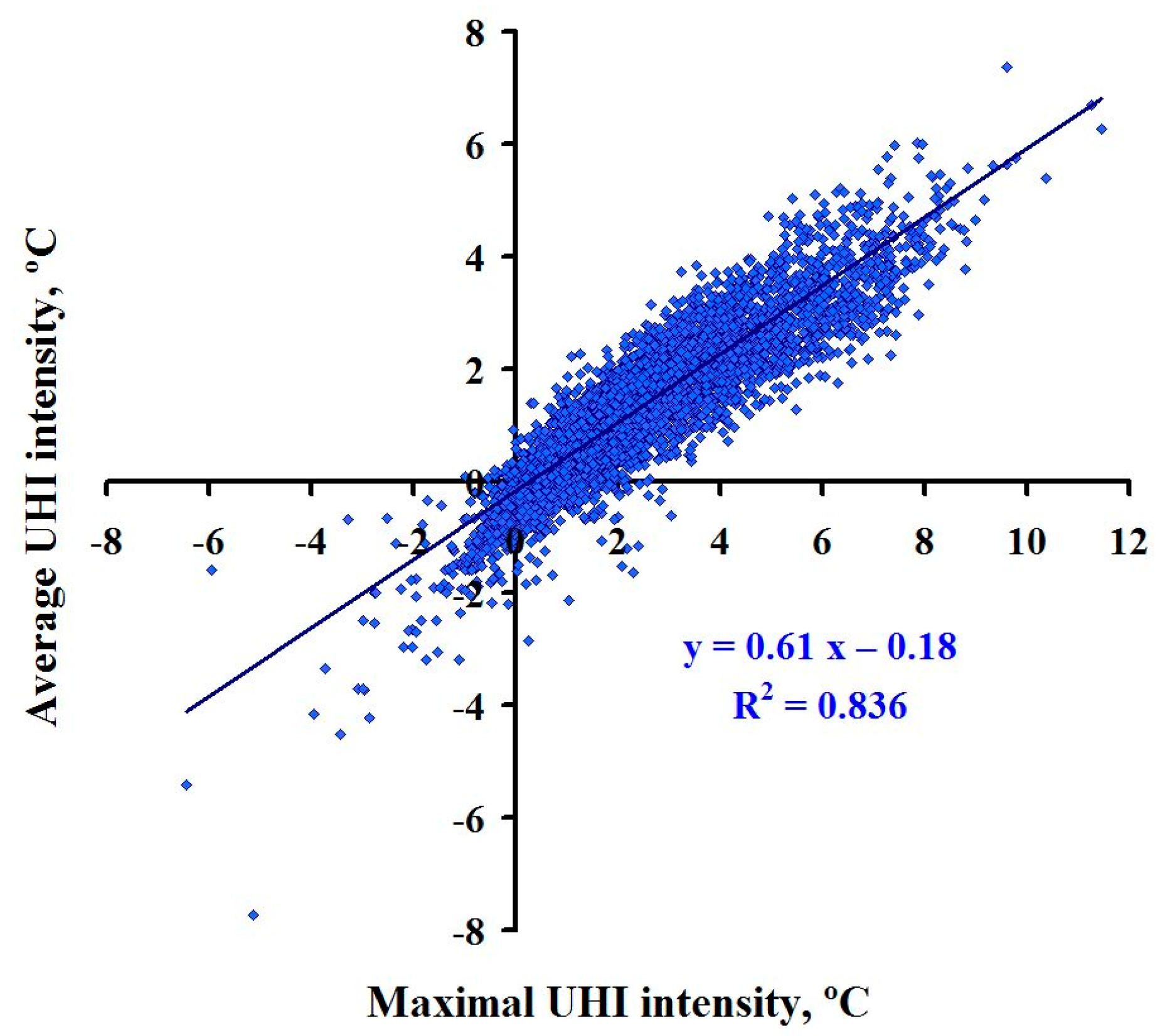
Both parameters are closely connected to each other. In Figure 1, all data about ΔT_MAX and ΔT_AV in Moscow for every 3 h during three years with a total data sampling of 8768 paired values are compared. As is seen from Figure 1, firstly, the statistical relation is close to linear, and secondly, it is very close: the correlation coefficient R is 0.91. It should be noted that the comparison of the mean daily values of ΔT_MAX and ΔT_AV for the same period from 2018 to 2020 with a total sampling of 1096 demonstrated almost the same result: 0.90 in Lokoshchenko and Alekseeva [7]. A small scatter of data is a result of changes in the thermal heterogeneity of Moscow area, i.e., changes in the differences between the data from the central station Balchug and the other four urban stations.

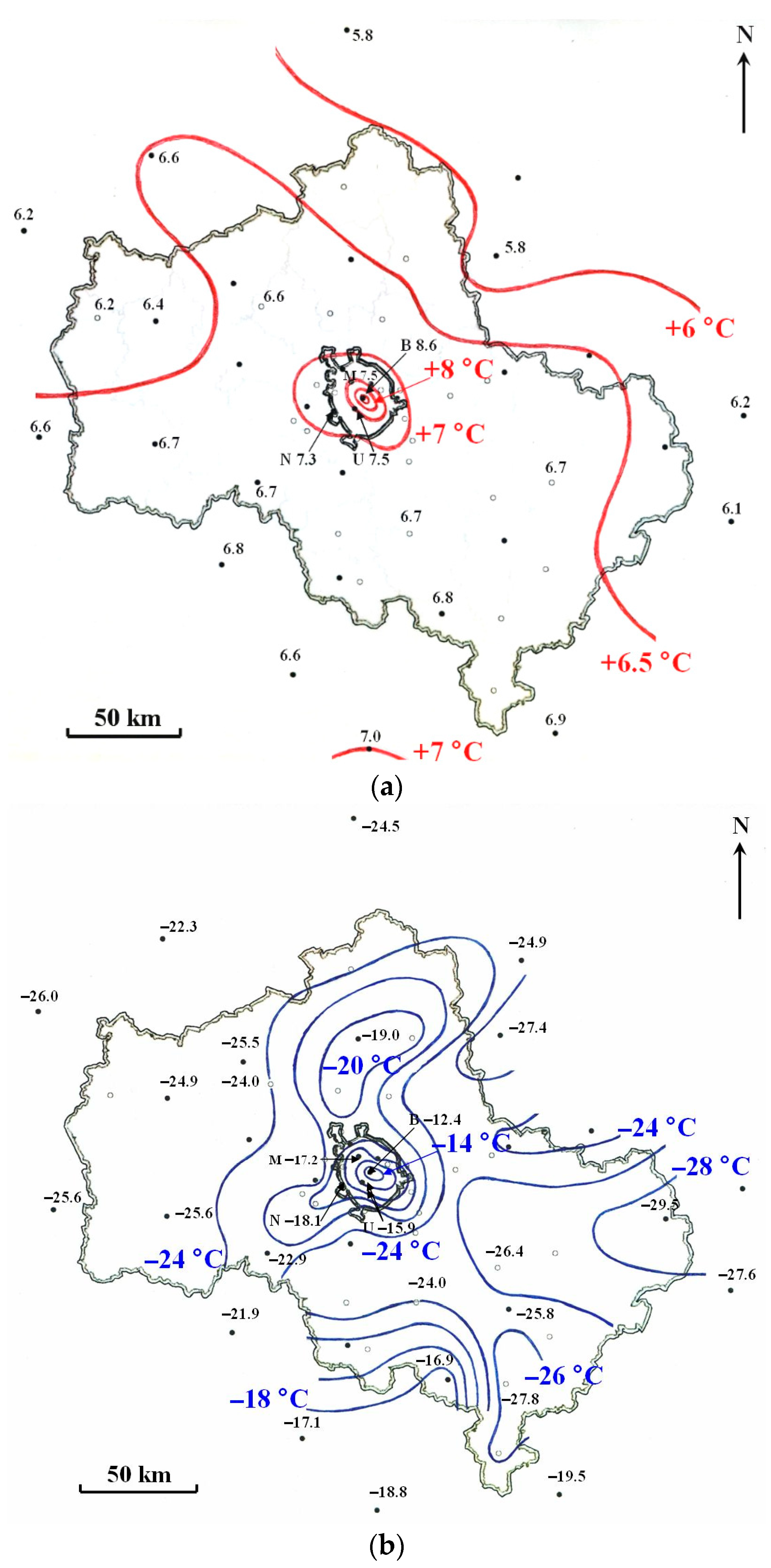
The map of isotherms calculated on average for the period 2018–2020 is presented in Figure 2a. It was compiled on the basis of 59 stations, including 8 weather stations in Moscow (5 manned weather stations and 3 automatic weather stations), 38 stations in rural zone of Moscow region (14 manned weather stations; 3 manned special stations at airports; 1 manned station in the nature reserve and 20 automatic weather stations) and an additional 13 manned weather stations in the neighboring areas of Moscow region. The black circles represent all manned weather stations with the most reliable data due to daily manned control. In contrast, automatic weather stations are shown as white circles; their data are complementary and less reliable. The isotherms in Figure 2a were drawn with a step of 0.5 °C by interpolation of values rounded to hundredths of °C; the same values on the map are rounded to tenths of °C.

As can be seen, the spatial field of the mean annual air temperature over Moscow region and neighboring areas is smoothed due to the thermal homogeneity of the relief (flat terrain and the absence of seacoasts). Except for Moscow city, only two isotherms (6.0 and 6.5 °C) are clearly present in rural zone in Figure 2a. One more isotherm (7.0 °C) appears only on the southern edge of the map according to the data from only one station (Tula). It should be noted that the shape of the isotherms (e.g., the ridge of the 6.5 °C isotherm extending to the northwest) may be not a real and time-stable climatic feature. The configuration of the isotherms depends both on the averaging period and on the number of weather stations whose data are available. For example, the spatial distribution of the mean annual T for earlier averaging periods (from 1951 to 1965 in Lokoshchenko and Isaev [24] and from 1957 to 1988 in Rubinshtein and Ginzburg [6]) was different. It should also be noted that the mean annual T sharply increased in recent decades due to the rapid climate warming: as can be seen, at present, the air temperature in rural areas of Moscow region ranges from 6 to 7 °C, while in the middle of the 20th century it was approximately 4 °C [24]. Geographical zonality is manifested in the general increase in T from the northeast to the southwest, but a large city (Moscow) disrupts it, creating a strong positive thermal anomaly. In the city centre T grew faster than in rural areas: from 5.6 °C on average for 1951–1965, up to 8.6 °C on average for 2018–2020. This was the result of the UHI accelerating in the recent past.

The UHI in Moscow is shown in Figure 2a by four closed isotherms from 7.0 to 8.5 °C. At the central Balchug (B) station, T is 8.6 °C, whereas at other urban manned stations, including the Meteorological observatory of Moscow State University, it ranges from 7.2 to 7.5 °C. Nemchinovka station, located close to the city margin (N), demonstrated a value in the same range, around 7.3 °C, while at other 37 rural stations, T during three years is, on average, 6.7 °C (from 6.0 to 7.3 °C). Thus, the maximal and average UHI intensities in Moscow for this period are 1.9 and 0.9 °C, respectively. Both estimates almost coincide with the average values for the period 2010–2014: 2.0 and 1.0 °C, respectively [8]. Therefore, Moscow UHI remains stable without any obvious changes in recent years. This could probably be the result of several reasons: the total stagnation of the Russian economy in the last decade, the deindustrialization of the city, its expansion in 2012 and, in addition, sharp drop in human activity in 2020 due to the COVID-19 pandemic. Firstly, as we know, the growth of gross domestic product in Russia has slowed down sharply since 2013. Secondly, over the past decade, many large industrial enterprises that created strong urban heat sources have been moved outside the city. In addition, in 2012, the so-called “New Moscow” was declared a new territory south of “Old Moscow”. Its gradual settlement led to a slowdown in growth, followed by a stabilization of population density in the traditional area of the city. Another additional reason was the strict quarantine measures during the COVID-19 pandemic, which led to the weakening of the UHI in Moscow in 2020 [7]. It should also be noted that the SUHI intensity in the field of T_S in Moscow on average for the period of 2008–2015 is 2.6 °C [23].

Let us also discuss an example of the extremely strong UHI that took place on 23 February 2018. As noted earlier by the authors [7], Moscow on that day was located in a low-gradient baric field close to the axis of an extended ridge. As a result, clear sky and calm were observed at most urban and rural weather stations at night (only a few stations in Moscow region recorded a slight cloudiness of 3/0, which means 30% coverage of the upper Ac clouds). On average, of eight readings for that day, ΔT_MAX and ΔT_AV were 7.4 and 4.4 °C, respectively. Late at night (at 3 a.m.), ΔT_MAX and ΔT_AV were even higher: 11.5 and 6.3 °C, respectively, because T was −10.8 °C at the central urban Balchug station; −16.0 °C on average at all five manned city stations; −22.3 °C on average for 13 manned rural stations.

It should be noted that the minimal T at that time was recorded at the Cherusti station in the east of Moscow region, −27.9 °C, so the maximal difference between the two stations in the region (Balchug and Cherusti) was 17.1 °C both at 3 a.m. local time and three hours later. Moreover, in the past, a similar extremely high difference in T between two stations in Moscow region was smaller: 13.6 °C on 26 March 2001, according to Lokoshchenko and Isaev [24]. Sometimes, these differences are taken as examples of an extremely strong UHI. However, they may be unreliable, because one rural station may reflect the influence of other factors: geographical zonality depending on the distance between stations, relief features (location of the station in a valley or basin), the passage of an atmospheric front between stations, etc. We note, in this regard, that Cherusti is the coldest weather station in the region: on average of three years, T there is the lowest among others: 5.0 °C. Thus, a correct estimation of the UHI intensity should be based on the real background T as a result of averaging over many rural stations.

The map of T at 6 a.m. on 23 February 2018 is presented in Figure 2b. At the next reading after 3 a.m., the ΔT_MAX was slightly lower (11.2 °C), while ΔT_AV, on the contrary, became higher than it was 3 h before: 6.7 °C. As can be seen, the T field is more heterogeneous than in Figure 2a due to one-time non-averaged data and, in addition, the specifics of the station location. Unlike Figure 2a, the isotherms in Figure 2b were drawn with a step of 2.0 °C. At Balchug station, T at 6 a.m. was −12.4 °C, while at other urban manned stations, it ranged from −15.9 to −21.0 °C. Thus, as seen in Figure 2b, the nocturnal UHI in Moscow in strong anticyclone conditions was presented by four closed isotherms inside the city (from −14 to −20 °C) and two semi-closed isotherms around it (−22 and −24 °C). Some additional features of the T spatial field, such as a minimum on the east (T was −29.5 °C at the Cherusti station) and a secondary maximum in the north, are probably associated with the influence of relief and other local factors.

A similar detailed mapping of isotherms showing either the average (over time) or maximal (over time) UHI intensity is presented for San Francisco, USA and for Karlsruhe, Germany in Kratzer [1]; for London, the UK, and other cities in Landsberg [2]; for Leicester, the UK, and other cities in Oke et al. [3]; for Vienna, Austria, in Böhm and Gabl [17], etc.

3.2. Statistical Analysis of the Influence of Meteorological Parameters on the UHI in Moscow

Let us discuss the influence of various meteorological parameters on the UHI intensity.

Table 1. Statistical relations between meteorological parameters and the UHI intensity. Moscow, 2018–2020. The first values are the correlation coefficients; second values in brackets are close to the correlation ratios. Bold values indicate the closest relations.

Parameter Which Can Influence the UHI	Sample Size	Average UHI Intensity	Maximal UHI Intensity
Total cloudiness, daily sum; 2018–2020	1096	−0.43 (0.45)	−0.54 (0.54)
Low cloudiness, daily sum; 2018–2020	1096	−0.56 (0.59)	−0.67 (0.70)
Mean daily wind speed at 15 m by the vane M-63 data, m/s; 2018–2020	1096	−0.39 (0.40)	−0.49 (0.50)
Mean daily wind speed in the 40–200 m air layer by the SODAR data, m/s; 2018–2019	729	−0.33 (0.34)	−0.41 (0.41)
Maximal daily wind speed among 8 values averaged over 10 min at 15 m by the vane M-63 data, m/s; 2018–2020	1096	−0.28 (0.29)	−0.33 (0.34)
Maximal wind gust during a day at 15 m by the vane M-63 data, m/s; 2018–2020	1096	−0.36 (0.37)	−0.36 (0.36)
Air temperature daily amplitude, °C; 2018–2020	1096	0.39 (0.47)	0.60 (0.64)
Surface temperature daily amplitude, °C; 2018–2020	1096	0.43 (0.49)	0.64 (0.68)
The highest air pressure during the day, hPa; 2018–2020	1096	0.37 (0.37)	0.29 (0.29)
The lowest relative humidity during the day, %; 2018–2020	1096	−0.42 (0.48)	−0.54 (0.59)
Precipitation amount, mm; 2018–2020	1096	−0.31 (0.38)	−0.28 (0.35)

summarizes and evaluates both linear and non-linear relationships for both ΔT_MAX and ΔT_AV with various meteorological parameters. Eleven parameters were taken into account: total and low cloudiness; four wind parameters (mean daily wind speed, maximal value of wind speed according to eight readings during the day, maximal daily wind gust at a height of 15 m according to M-63 data and mean daily wind speed in the 40–200 m air layer according to MODOS sodar data); daily amplitudes of air and surface temperatures; the highest air pressure, the lowest relative humidity and precipitation amount during the day. Evidently, only cloudiness, wind parameters and possibly precipitation may directly affect the UHI intensity. 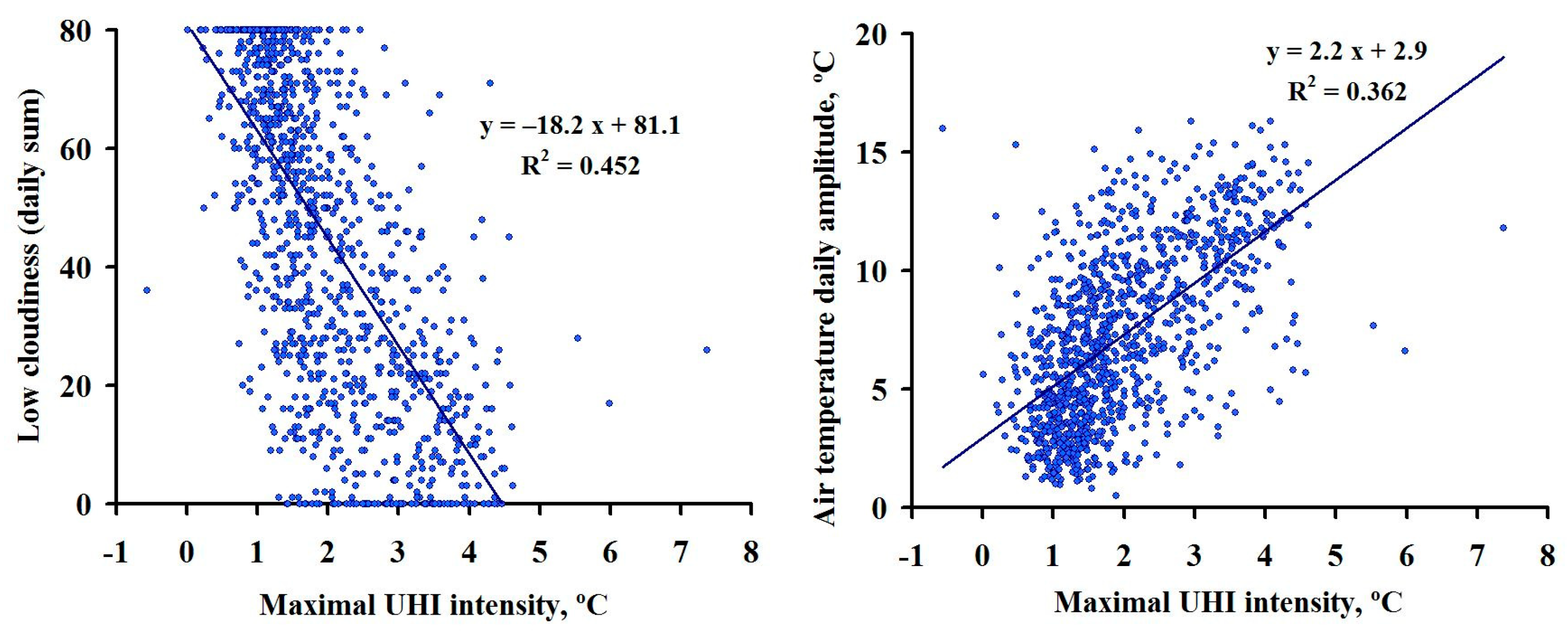The T and T_S amplitudes indirectly indicate anticyclonic conditions; relative humidity indirectly reflects changes in T. As we know a priori, the highest air pressure is not a real indicator of anticyclonic conditions; nevertheless, it was also analyzed. Two examples of the closest relations are presented in Figure 3.

In addition to the classical Pearson correlation coefficient R indicating a linear relation, it was also necessary to check for possible non-linear relations. For this, the confidence index R² of their description by the 4th degree power functions was used. The square root of this index was conventionally taken as the correlation ratio η. In fact, such a high order of the function allows us to take its confidence index as a value very close to η² (the confidence indexes for the 4th, 5th and 6th degrees power functions are almost the same for all parameters). The closer to a linear relation, the closer R² and η² are to each other. For all parameters, it was determined that (η²–R²) is <0.1, except for only one comparison between ΔT_AV and T daily amplitude, where the obtained value is 0.12. For all other parameters, the maximal value of (η²–R²) is only 0.06 for ΔT_AV and 0.07 for ΔT_MAX. Thus, except for just one relation, the non-linearity is negligibly small, so that R is a real indicator of the closeness of the relation.

As can be seen, low cloudiness represents the closest relation with the UHI intensity. The UHI intensity is more closely related to low cloudiness than to total cloudiness. This is not surprising, since the effect of thin and rarefied upper-level clouds (Ci and others) on the surface radiation balance is comparatively weak. As shown in [7], the relationship between the UHI intensity and cloudiness is especially strong at night, when the role of low cloudiness in the radiation and heat balances of the surface is much higher than in the daytime. On the contrary, a separate comparison of ΔT_MAX and ΔT_AV with low cloudiness only for 3 p.m. leads to insignificant (<0.1) values of R, which is also not surprising, since the contribution of counter radiation to the daytime radiation balance is small.

Only slightly smaller values of R and η values were obtained for the relations with the daily amplitude of the surface temperature T_S, the daily amplitude of the air temperature T, total cloudiness and the lowest relative humidity during the day. The relations of the UHI intensity with various wind speed parameters are weaker, especially for wind speeds at high altitudes, while the relationships of the UHI intensity with the highest air pressure and precipitation are weak. A similar result on the weakening of the relationship between the UHI intensity and V with increasing altitude when comparing data at a height of 90 and 252 m was obtained in Vienna, Austria, in Böhm and Gabl [17]. Thus, the wind speed affects the UHI intensity in Moscow less than cloudiness, in contrast to the conditions of Ibadan, Nigeria according to Anibaba et al. [16].

To test the significance of statistical relationships, the well-known Student’s t-criterion is often used:

$$t=\frac{R}{{\sigma }_R},{\sigma }_R=\frac{\sqrt{1-R^2}}{\sqrt{n-2}}$$

(3)

where R is Pearson correlation coefficient; σ_R is the R error; n is the sample size. As we know, the relation may be considered significant if t > 3. As can be seen from

Table 2. Checking the statistical significance of the relationship between meteorological parameters and UHI intensity. Moscow, 2018–2020. The first values are t-test values; the second ones in brackets are the z-test values. Bold values indicate the closest relations.

Parameter Which Can Influence the UHI	Sample Size	Average UHI Intensity	Maximal UHI Intensity
Total cloudiness, daily sum; 2018–2020	1096	−15.9 (−15.4)	−21.0 (−19.8)
Low cloudiness, daily sum; 2018–2020	1096	−22.1 (−20.7)	−30.0 (−26.9)
Mean daily wind speed at 15 m by the vane M-63 data, m/s; 2018–2020	1096	−13.8 (−13.5)	−18.5 (−17.7)
Mean daily wind speed in the 40–200 m air layer by the SODAR data, m/s; 2018–2019	729	−9.4 (−9.2)	−12.1 (−11.7)
Maximal daily wind speed among 8 values averaged over 10 min at 15 m by the vane M-63 data, m/s; 2018–2020	1096	−9.7 (−9.6)	−11.4 (−11.2)
Maximal wind gust during a day at 15 m by the vane M-63 data, m/s; 2018–2020	1096	−12.7 (−12.4)	−12.7 (−12.4)
Air temperature daily amplitude, °C; 2018–2020	1096	13.9 (13.5)	24.6 (22.8)
Surface temperature daily amplitude, °C; 2018–2020	1096	15.8 (15.3)	27.7 (25.2)
The highest air pressure during the day, hPa; 2018–2020	1096	13.1 (12.8)	10.1 (10.0)
The lowest relative humidity during the day, %; 2018–2020	1096	−15.4 (−14.9)	−21.5 (−20.2)
Precipitation amount, mm; 2018–2020	1096	−10.7 (−10.5)	−9.8 (−9.6)

, according to Student’s criterion, even the weakest relations are significant with an extremely high probability (much higher than 0.999). It should be noted that the t criterion is parametric and can be used if the distribution follows the Normal law. As shown by the authors in [7], the distributions of the UHI intensity are close to the Normal law in summer, while in winter they have a significant positive asymmetry. However, for large (n > 100) samples and R values far from 0 and 1, its application is possible even without a special estimation of the type of distribution according to Isaev [25]. Thus, given the large sample size even for sodar data about wind, we use the t-criterion correctly. However, for greater confidence in the conclusions, we also consider another non-parametric Fisher’s z-criterion:

$$t_z=\frac{Z}{{\sigma }_z},\mathrm{where}Z\approx \frac{1}{2}\cdot \ln \frac{1+R}{1-R},{\sigma }_z=\frac{1}{\sqrt{n-3}}$$

(4)

As can be seen from Table 2, all absolute values of t_z are only a bit lower than absolute values of t. All correlation coefficients according to the z-criterion (4) are also reliable with an extremely high probability at a significance level α→0 close to zero. Thus, any of the considered meteorological parameters significantly affect the UHI intensity.

In addition to the usual Pearson correlation coefficients, a multiple correlation coefficient R_X·YZ was also calculated between the maximal UHI intensity (X) and the two parameters which affect it more strongly than all other ones: low cloudiness (Y) and the mean daily wind speed at 15 m (Z). As we know, this coefficient indicates the simultaneous dependence of X on both parameters Y and Z, i.e., the closeness of a linear correlation between the maximal UHI intensity and the combined effect of both low cloudiness and mean daily wind speed. On average, over three years, it was determined to be 0.76. It should be noted that a separate calculation of the same R_X·YZ only for the data of 2018 leads to its even higher value: 0.82. It is notable that similar multiple correlation coefficient between the UHI intensity, wind speed and cloudiness in Vienna was much lower: only from 0.40 to 0.47 according to Böhm and Gabl [17]. It may be that they used the data on total cloudiness and, therefore, the relation was weaker.

As is known, the significance of the multiple correlation coefficient is estimated by the Fisher distribution F with 2 and (n − 3) degrees of freedom and under the null hypothesis that this coefficient is equal to zero in accordance with

$$\frac{R_{X\cdot YZ}^2}{1-R_{X\cdot YZ}^2}\cdot \frac{n-3}{2}<F_{\alpha ,2,n-3}$$

(5)

In our case, the values of the formula are 729 for a three-year period and 372 for 2018, while the critical values of the Fisher statistics, even for a significance level of α = 1%, are 4.63 and 4.67, respectively. Thus, the significance of the R_X·YZ values is evident for α→0.

3.3. Empirical Functions of Meteorological Parameters

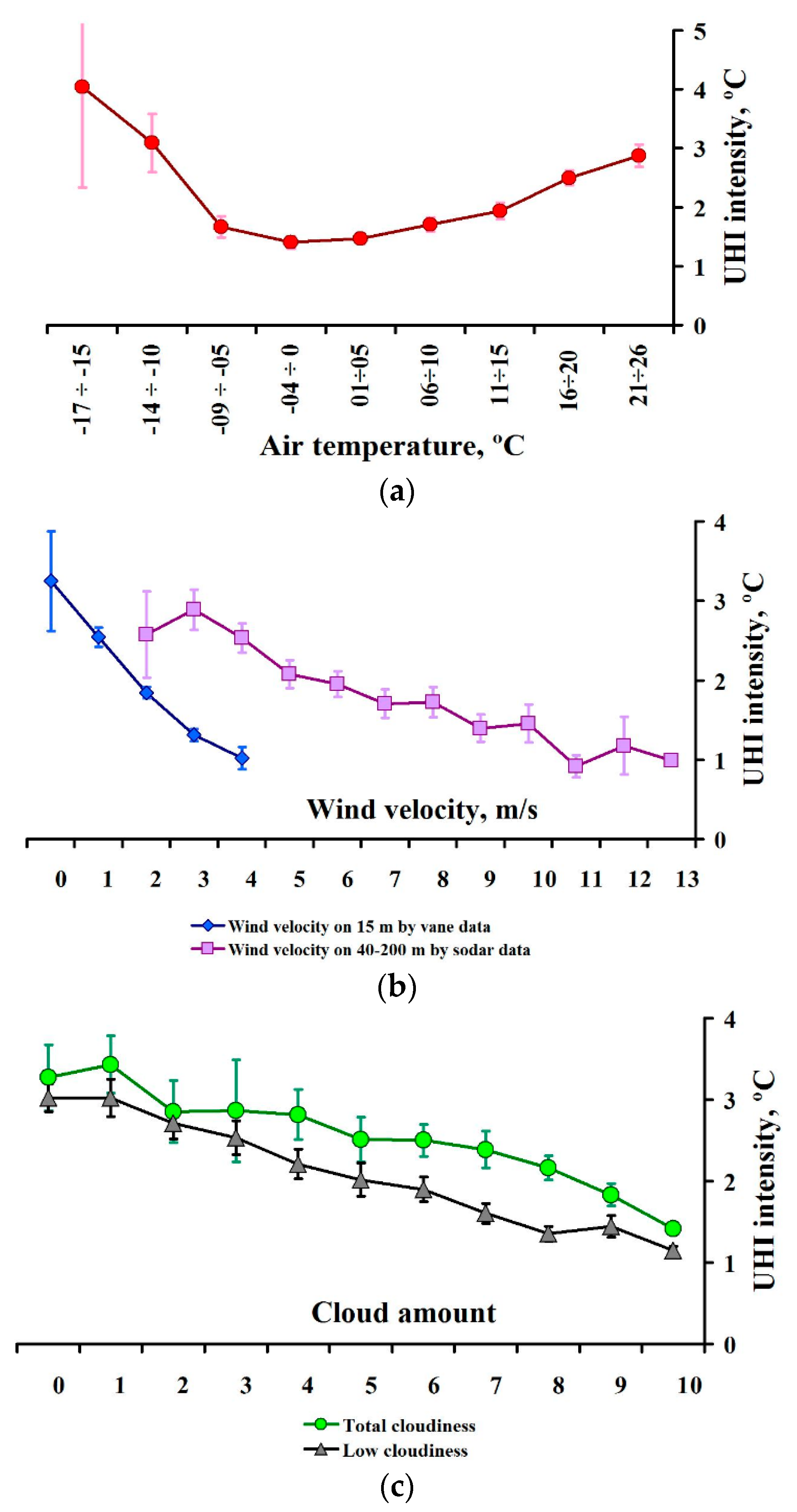
Let us discuss the UHI intensity functions of the main meteorological parameters (air temperature T, wind speed V, total and low cloudiness). Such empirical statistical dependencies, calculated on large data samples, allow a better understanding of the influence of various parameters on the generation and dynamics of the UHI. As above, we used the same UHI intensity data and measurement results at the MSU Meteorological observatory for three years (from 2018 to 2020). All values of the UHI intensity, T, V and cloud amounts were averaged for each day. Thus, we do not consider any changes in the daily course, since they can create some noise in the results due to the inertia of the UHI response to short-term changes in meteorological parameters. Evidently, the use of daily averaged values provides more reliable functions, but, on the other hand, leads to shorter ranges of all parameters. Here, we used the maximal UHI intensity, i.e., ΔT_MAX values (the difference between the Balchug station and the average of 13 out of 14 rural stations in Moscow region, except for Nemchinovka).

As seen in Figure 4a, the function of the UHI intensity of T based on 1096 daily averaged values is non-monotonous is the demonstration of a minimum of the UHI intensity in the middle of the T range: from −4 to 0 °C. Relatively low values are observed in a wider range of T: from −9 to +10 °C. Both at higher and lower T values, the UHI intensity grows so much that there are two of its maxima at the edges of the function: at −15…−17 °C and at 21–26 °C.

Evidently, extremely low and extremely high T values when the UHI is the strongest are associated with anticyclonic conditions in winter and in summer. Neighboring ranges (−9…0 °C and 11–15 °C) on average indicate a much weaker UHI and represent either cyclonic or mixed conditions in winter and summer, respectively. Intermediate values of T from −4 to +10 °C in the middle of the total range are usually observed in the transitional seasons (spring and autumn), when the thermal difference between cyclonic and anticyclonic conditions is not so clear.

As can be seen, severe frosts increase the heat island faster than extreme heat. A stronger UHI in the conditions of extremely low T in winter than in hot weather in summer may seem unexpected, since, as we know, the UHI intensity annual course on average has a maximum in summer according to Lokoshchenko and Alekseeva [7]. However, this is not surprising, because a cold wave in European Russia in recent decades has been a much rarer phenomenon than a heat wave. Data sampling for the lowest T values is insufficient: there were 33 days with mean daily T from −14 to −10 °C, but only 3 days with T from −17 to −15 °C.

On the contrary, the sample of data on warm and hot weather in Moscow for 3 years is much larger: 214 days at 16–20 °C and 97 days at 21–26 °C. Indeed, as in Lokoshchenko and Alekseeva [7], during a short period of severe frosts under anticyclone conditions in February 2018, the UHI intensity was above average in summer. It should also be noted that differences in the UHI intensity between near-zero and extremely low T, as well as between near-zero and extremely high T, are statistically significant at a 5% significance level.

A similar analysis was carried out for the UHI intensity function of the wind speed V (Figure 4b). This function was calculated twice, both according to the data of the M-63 vane at a height of 15 m above the ground, and according to the MODOS sodar data on V in the air layer from 40 to 200 m. Station data on V were used for all three years (1096 daily averaged values), while sodar data were only used for two years (2018 and 2019) and their sample contains 729 daily values, since one day (22 September 2018) was lost to acoustic remote sensing: the sodar was not working.

All station data on wind speed according to M-63 measurements were averaged over eight values every 3 h during the day. The V range of these daily averaged data is short, since the wind speed in the surface air layer is limited. The highest value was 4.6 m/s and was observed three times when Moscow was located on the periphery of deep cyclones under conditions of a high horizontal baric gradient: 19 December 2019; 13 March; and 22 April 2020. The lowest V close to calm was 0.2 m/s and was observed twice for two days in a row: on 8 and 9 September 2018, under conditions of a low-gradient baric field on the periphery of an extensive anticyclone.

Therefore, all values according to M-63 data were divided into five gradations. Sample data comprised 12 days for 0–1 m/s; 297 days for 1–2 m/s; 595 days for 2–3 m/s; 172 days for 3–4 m/s and 20 days for the highest values of 4–5 m/s. As is seen, the UHI intensity function of V according to the M-63 data is simple and monotonously decreasing. It is notable that this function is strong: starting from the second gradation of 1–2 m/s, the average UHI intensity in each next gradation is significantly lower than that in the previous one with the 0.95 confidence probability. It should also be noted that this function is non-linear and tends to slow down as V increases. Thus, it is qualitatively close to a hyperbola (inverse proportionality function) y = k/x for x > 0.

Another calculation was conducted using daily averaged sodar wind speed data in the air layer 40–200 m above the ground. As can be seen, in general, this function also demonstrates a gradual decrease in the UHI intensity with wind increase, but weaker than the previous function based on the M-63 data. This is not surprising, since the higher the air layer above the ground, the weaker the effect of the high-altitude wind on T near the ground. Differences between average values of the UHI intensity are statistically significant only when comparing conditions of light (V ≤ 6 m/s) and very strong winds (V ≥ 9 m/s). Unlike the function of the M-63 data, the differences between adjacent gradations of sodar data are, as a rule, insignificant. In the range of intersection of both functions from 2 to 4 m/s, the UHI intensity is much higher according to the sodar data than according to the M-63 data due to the total increase in the wind with a height. The sampling size of the MODOS data is quite sufficient for statistical analysis (≥24 cases) at all gradations, except for the three highest gradations (from 11 to 13 m/s). Nevertheless, we can assume that the stabilization of the UHI intensity under strong winds for V >10 m/s at these gradations is a real effect, as is the deceleration of the fall of the previous function according to the M-63 data for V values from 3 to 4 m/s (this range is insufficient for the asymptotic low limit detection). A similar function with a deceleration of the UHI intensity fall for V > 4.5 m/s was obtained in Shanghai by Qunfang Huang et al. [14], for V > 3.5 m/s, in the cities of the Pearl River Delta by Baomin Wang et al. [15].

Indeed, if the range of wind speed is not too short, then at a certain threshold value of V its influence on the UHI reduces to nothing. This critical value of V according to station (close to the ground) data preventing the development of the UHI was obtained as 7 m/s in Ibadan, Nigeria by Anibaba et al. [16]; 6 m/s in Salamanca, Spain by Alonso et al. [18]; 5 m/s in both Szeged, Hungary by Unger [12], and Melbourne, Australia by Morris et al. [13]. Evidently, taking into account the general increase in wind with a height in the atmospheric boundary layer, the 10 m/s threshold of wind influence in the 40–200 m air layer corresponds to a lower threshold at the station level (usually 10–15 m), which seems to be close to these estimations.

Empirical functions of the UHI intensity on cloudiness (both total and low) are presented in Figure 4c. As can be seen, in general, both functions decrease with increasing cloudiness, so the most favorable condition for the UHI is a clear sky. Differences between the UHI intensity for ≥90% and <90% of total cloudiness and for ≥70% and <70% of low cloudiness are statistically significant with a 0.95 confidence probability. Another conclusion is that the difference between the effect of total and low cloudiness on the UHI is stronger the higher the cloudiness: it is insignificant at cloud cover <50% and significant at >50%. Similar UHI intensity functions of cloudiness were obtained in Unger [12] for Szeged, in Qunfang Huang et al. [14] for Shanghai, in Morris et al. [13] for Melbourne.

4. Conclusions

In recent years, the mean annual air temperature in rural zone of Moscow region has ranged from 6 to 7 °C. This means that the regional climate has become ~2 °C warmer than it was 60–70 years ago. In the centre of Moscow, warming occurred faster than outside the city.

The maximal in-space urban heat island UHI intensity (comparison of the city centre with rural zone) in Moscow has averaged 1.9 °C in recent years; the average in-space intensity (comparison of the entire urban zone with the rural one) is 0.9 °C. In recent years, the UHI intensity in Moscow has stabilized rather than increased as before, probably due to deindustrialization and expansion of the city and also due to a drop in human activity during the COVID-19 pandemic lockdown. In the case of a strong anticyclone, the maximal in-space and -time UHI intensity can reach 11–12 °C.

Low cloudiness and daily air/surface temperature amplitude (the latter parameter indirectly indicates anticyclone conditions) demonstrate the closest relations with the UHI intensity with Pearson’s correlation coefficient and correlation ratio up to −0.67 and 0.70, respectively, for low cloudiness and the maximal UHI intensity. The relationship between the UHI intensity and mean daily wind speed and total cloudiness is slightly weaker. All relations are close to linear (nonlinearity is small) and statistically significant. The relations of all meteorological parameters with the maximal in space UHI intensity are closer than with the average in-space UHI intensity. The multiple correlation coefficient between the maximal UHI intensity and the two parameters (low cloudiness and wind speed) is approximately 0.8.

The UHI intensity function of air temperature has a minimum in the middle range from −4 to 0 °C; it increases at both lower and higher T due to the influence of anticyclonic conditions. The UHI intensity function of the wind speed decreases with the wind strength and weakens with height. The threshold value of the wind speed (resulting in a minimum of the UHI function) is approximately 10 m/s at a height of 40–200 m. The UHI intensity functions of both total and low cloudiness also decrease with increasing cloudiness, and the difference between the effect of total and low cloudiness on the UHI intensity is statistically significant at over 50% cloudiness.

References

1. Kratzer, P.A. Das Stadtklima (The Urban Climate); Friedr. Vieweg and Sohn: Braunschweig, Germany, 1956; p. 221. [Google Scholar]
2. Landsberg, H.E. The Urban Climate; Academic Press: New York, NY, USA, 1981; p. 275. [Google Scholar]
3. Oke, T.R.; Mills, G.; Christen, A.; Voogt, J.A. Urban Climates; University Press: Cambridge, UK, 2017; 525p. [Google Scholar]
4. Bogolepow, M.A. Über das Klima von Moskau. Meteorologische Z. 1928, XLV, 152–154. (In German) [Google Scholar]
5. Kislov, A.V. (Ed.) Climate of Moscow under Global Warming; Izd. MGU: Moscow, Russia, 2017; 288p. (In Russian) [Google Scholar]
6. Rubinshtein, K.G.; Ginzburg, A.S. Estimation of air temperature and precipitation changes in large cities (on example of Moscow and New York). Russ. Meteorol. Hydrol. 2003, 28, 20–26. [Google Scholar]
7. Lokoshchenko, M.A.; Alekseeva, L.I. About the Annual Course of Moscow Heat Island and the Impact on It of the Quarantine Measures to Prevent the COVID-19 Pandemic in 2020. Izvestiya. Atmos. Ocean. Phys. 2022, 58, 168–177. [Google Scholar] [CrossRef]
8. Lokoshchenko, M.A. Urban heat island and urban dry island in Moscow and their centennial changes. J. Appl. Meteorol. Climatol. 2017, 56, 2729–2745. [Google Scholar] [CrossRef]
9. Kadygrov, E.N.; Kuznetsova, I.N.; Golitsyn, G.S. Heat island in the boundary atmospheric layer over a large city: New results based on remote sensing data. Doklady Earth Sci. 2002, 385A, 688–694. [Google Scholar]
10. Lokoshchenko, M.A.; Korneva, I.A.; Kochin, A.V.; Dubovetsky, A.Z.; Novitsky, M.A.; Razin, P.Y. Vertical Extension of the Urban Heat Island above Moscow. Doklady Earth Sci. 2016, 466, 70–74. [Google Scholar] [CrossRef]
11. László, E.; Bottyán, Z.; Szegedi, S. Long-term changes of meteorological development in the region of Debrecen, Hungary. Theor. Appl. Climatol. 2016, 124, 365–373. [Google Scholar] [CrossRef]
12. Unger, J. Heat Island intensity with different meteorological conditions in a medium-sized town: Szeged, Hungary. Theor. Appl. Climatol. 1996, 54, 147–151. [Google Scholar] [CrossRef]
13. Morris, C.J.G.; Simmonds, I.; Plummer, N. Quantification of the influences of wind and cloud on the nocturnal urban heat island of a large city. J. Appl. Meteorol. 2001, 40, 169–182. [Google Scholar] [CrossRef]
14. Huang, Q.; Li, L.; Lu, Y.; Yang, Y.; Li, M. The roles of meteorological parameters in Shanghai’s nocturnal urban heat island from 1979 to 2013. Theor. Appl. Climatol. 2020, 141, 285–297. [Google Scholar] [CrossRef]
15. Wang, B.; Ding, S.; Qiao, G.; Guo, Y.; Wu, Y. Study on the Urban Heat Islands and the Meteorological Elements over the Pearl River Delta. In Proceedings of the the 9th ICUC (International Conference on Urban Climate jointly with 12th Symposium on the Urban Environment), Toulouse, France, 20–24 July 2015. [Google Scholar]
16. Anibaba, B.W.; Durowoju, O.S.; Adedeji, O.I. Assessing the significance of meteorological parameters to the magnitude of urban heat island (UHI). An. Univ. Din Oradea Ser. Geogr. 2019, XXIX, 30–39. [Google Scholar] [CrossRef]
17. Böhm, R.; Gabl, K. Die Wärmeinsel einer Großstadt in Abhängigkeit von verschiedenen meteorologischen Parametern. Arch. Meteorol. Geophys. Bioclimatol. Ser. B 1978, 26, 219–237. (In German) [Google Scholar] [CrossRef]
18. Alonso, M.S.; Fidalgo, M.R.; Labajo, J.L. The urban heat island in Salamanca (Spain) and its relationship to meteorological parameters. Clim. Res. 2007, 34, 39–46. [Google Scholar] [CrossRef]
19. Lee, S.-H.; Baik, J.-J. Statistical and dynamical characteristics of the urban heat island intensity in Seoul. Theor. Appl. Climatol. 2010, 100, 227–237. [Google Scholar] [CrossRef]
20. Li, L.; Zha, Y.; Wang, R. Relationship of surface urban heat island with air temperature and precipitation in global large cities. Ecol. Indic. 2020, 117, 106683. [Google Scholar] [CrossRef]
21. Bespalov, D.P. (Ed.) Instructions for hydrometeorological stations and posts: Part I. Gidrometeoizdat Rep. 1969, 3, 307. (In Russian) [Google Scholar]
22. Reifer, A.B.; Alexeyenko, M.I.; Burtsev, P.N.; Zastenker, A.I.; Belogurov, Y.A.; Nepomnyashchiy, S.I. Handbook on Hydrometeorological Instruments and Systems; Gidrometeoizdat: Leningrad, Russia, 1971; p. 372. (In Russian) [Google Scholar]
23. Lokoshchenko, M.A.; Enukova, Y. A. Urban Heat Island in Moscow Derived from Satellite Data. Russ. Meteorol. Hydrol. 2020, 45, 488–497. [Google Scholar] [CrossRef]
24. Lokoshchenko, M.A.; Isaev, A.A. Influence of Moscow city on the air temperature in Central Russia. In Proceedings of the 5th ICUC (International Conference on Urban Climate), Poland, Lodz, 1–5 September 2003; Volume 2, pp. 449–453. [Google Scholar]
25. Isaev, A.A. Statistics in Meteorology and Climatology; Izd. MSU: Moscow, Russia, 1988; 248p. (In Russian) [Google Scholar]
Figure 1. Statistical relation between the maximal and average UHI intensities in Moscow for every 3 h during 2018–2020.
Atmosphere 14 00507 g001
Figure 2. Air temperature maps over Moscow region. (a) Mean isotherms on average for the period 2018–2020; (b) Isotherms on 23 February 2018, at 06 a.m. Margins of Moscow city (until 2012) and Moscow region are shown by double black lines. Manned and automatic weather stations are shown by black and white circles, respectively. B—Balchug station; M—Mikhelson observatory; U—MSU MO; N—Nemchinovka station.
Atmosphere 14 00507 g002
Figure 3. Graphs of statistical relations between the maximal UHI intensity, low cloudiness (left) and daily air temperature amplitude (right). Moscow, 2018–2020.
Atmosphere 14 00507 g003
Figure 4. Empirical functions of the UHI intensity of daily averaged meteorological parameters in 2018–2020, Moscow. (a) Function of the air temperature; (b) functions of the wind velocity; (c) functions of the cloudiness. Confidence intervals are calculated with the 0.95 confidence probability.
Atmosphere 14 00507 g004