Study of the Dynamical Relationships between PM2.5 and PM10 in the Caribbean Area Using a Multiscale Framework

Abstract

The Caribbean basin is a geographical area with a high prevalence of asthma due to mineral dust. As such, it is crucial to analyze the dynamic behavior of particulate pollutants in this region. The aim of this study was to investigate the relationships between particulate matter with aerodynamic diameters less than or equal to 2.5 and 10 μm (PM2.5 and PM10) using Hilbert–Huang transform (HHT)-based approaches, including the time-dependent intrinsic correlation (TDIC) and time-dependent intrinsic cross-correlation (TDICC) frames. The study utilized datasets from Puerto Rico from between 2007 and 2010 to demonstrate the relationships between two primary particulate matter concentration datasets of air pollution across multiple time scales. The method first decomposes both time series using improved complete ensemble empirical mode decomposition with adaptive noise (ICEEMDAN) to obtain the periodic scales. The Hilbert spectral analysis identified two dominant peaks at a weekly scale for both PM types. High amplitude contributions were sustained for long and continuous time periods at seasonal to intra-seasonal scales, with similar trends in spectral amplitude observed for both types of PM except for monthly and intra-seasonal scales of six months. The TDIC method was used to analyze the resulting modes with similar periodic scales, revealing the strongest and most stable correlation pattern at quarterly and annual cycles. Subsequently, lagged correlations at each time scale were analyzed using the TDICC method. For high-frequency PM10 intrinsic mode functions (IMFs) less than a seasonal scale, the value of the IMF at a given time scale was found to be dependent on multiple antecedent values of PM2.5. However, from the quarterly scale onward, the correlation pattern of the PM2.5-PM10 relationship was stable, and IMFs of PM10 at these scales could be modeled by the lag 1 IMF of PM2.5. These results demonstrate that PM2.5 and PM10 concentrations are dynamically linked during the passage of African dust storms.

1. Introduction

With global urbanization and industrialization, particulate matter has become one of the most significant components of atmospheric pollutants [1]. Particulate matter in different forms can have a significant impact on climate [2,3], and can induce adverse health effects, such as respiratory and cardiovascular diseases [4,5,6]. Researchers have extensively studied the relationship between particulate matter and meteorological parameters, with most studies reporting multiscale characteristics of this behavior [7,8]. Particulate matter with aerodynamic diameters less than or equal to 2.5 and 10 $\mathsf{\mu }$m ($PM2.5$ and $PM10$) are among the most referenced particulate pollutants in the literature [9,10,11,12].

In the field of air pollutants, $PM2.5$ and $PM10$ often exhibit non-linear and non-stationary behavior, showing the coexistence of different spatial–temporal scales [13,14,15,16]. Li et al. [17] used a seasonal-trend decomposition procedure based on LOESS (STL) coupled with a wavelet analysis to conduct a spatial–temporal analysis of the Air Pollution Index (API) and its relationship with meteorological factors in Guangzhou, China, from 2001 to 2011. They found a negative relationship between API, temperature, relative humidity, precipitation, and wind speed, and a positive relationship between API, the diurnal temperature range, and atmospheric pressure in the annual cycle. Fu et al. [18] analyzed the association between $PM2.5$ and other pollutants, such as O${}_3$, CO, SO${}_2$, NO${}_2$, in China, in addition to different meteorological parameters, considering the 2014–2018 datasets of daily and monthly scales, using the ensemble empirical mode decomposition (EEMD). In general, most of the past studies independently examined the association between $PM2.5$ and $PM10$ with the meteorological factors or concentrations of other pollutants.

Apart from such studies, it is highly important to assess the mutual association between the two pollutants to accurately model air pollutants. Filonchyk et al. [19] investigated a linear association between $PM2.5$ and $PM10$ in 11 cities of Gansu Province in 2015. Munir et al. [20] examined the association between $PM2.5$ and $PM10$ and their relationship with meteorological parameters in Makkah, Saudi Arabia. The Caribbean basin is a strategically important area for studying the impacts of mineral dust on $PM2.5$–$PM10$ behavior because it is an intermediate zone located between the Caribbean Sea and the Atlantic Ocean with low anthropogenic activity, in contrast to megacities [21]. It is well known in the literature that this area is frequently affected by the major long-range Saharan dust transportation from West African desert sources [22,23,24,25,26,27].

Atmospheric circulation conditions drive the transport of mineral aerosols across the Atlantic towards the Lesser Antilles, which are mostly affected by desert dust plumes from May to August, constituting the high dust season for Caribbean islands. Outside of this period, dust episodes are significantly less frequent [23,28,29,30]. The intensity and frequency of dust events strongly depend on the distance from African coasts and the phenomenon of dust particle loss all along the route of dusty air masses. This factor significantly reduces air quality and results in a significant increase in the concentrations of $PM10$ and $PM2.5$ measured in the surface layer of the atmospheric boundary layer [31]. $PM10$ particles are mainly representative of the size range of Saharan dust particles from sand haze episodes, while $PM2.5$ particles are less representative of desert aerosols. However, in this geographical area, only a few studies have investigated the behavior of $PM2.5$ and $PM10$ simultaneously, and all their results are based solely on statistical methods [32,33,34].

Even though the relationship between $PM2.5$ and $PM10$ has been studied, the multiscale correlation between these pollutants has not yet been fully investigated. In this paper, a multiscale decomposition framework is used to dynamically investigate the relationship between $PM2.5$ and $PM10$. The EMD method, which is an adaptive time-frequency data analysis technique, was first introduced by Huang et al. [35]. Its objective is to decompose any time series into a sum of different intrinsic mode functions (IMFs) through a sifting procedure [36,37]. Although this method has revolutionized the understanding of physical processes, it may introduce a serious drawback known as the mode mixing problem [38]. The mode mixing problem comes about when very similar oscillations are present in different modes [39]. Wu and Huang [40] proposed the EEMD technique, which involves adding white noise series to the original time series to aid in the sifting process and prevent mode mixing. However, this method does not completely eliminate white noise during the reconstruction of the time series [41]. Thus, Torres et al. [42] introduced the complete EEMD with adaptive noise (CEEMDAN) approach, which attempts to reduce residual noise in the modes. However, this method can still introduce spurious modes and noisy components in the early stages of the decomposition. To address these issues, Colominas et al. [43] proposed the improved CEEMDAN (ICEEMDAN), which is designed to produce components with less noise and more physical meaning.

The time-dependent intrinsic correlation (TDIC) analysis is a multiscale correlation method based on the EMD method or its variants to assess the correlation between two time series [44]. In the literature, the TDIC method has often been used to investigate the relationship between a pollutant and meteorological parameters [7,8,45,46]. In the Caribbean area, African dust storms have strong impacts on solar radiation ($SR$), air temperature (T), wind speed (U), rainfall (R), and visibility (V) [7,8]. During the high dust season, $PM10$ is positively and negatively correlated, respectively, to $SR$-T-U and R-V. The correlations between $PM10$ and $PM2.5$ evolve over time depending on the duration and intensity of dust events. However, to our knowledge, no study has used the multiscale decomposition framework to analyze the relationship between these two pollutants. In addition to the popular TDIC analysis [47,48,49,50,51,52,53,54], the lagged influence of correlations also needs to be analyzed for developing predictive models with improved accuracy. This can be achieved using the time-dependent intrinsic cross-correlation (TDICC) approach [55,56]. Therefore, the aims of this study are (i) to investigate the multiscale periodic features of $PM10$ and $PM2.5$ using ICEEMDAN, (ii) to find the multiscale association between $PM10$ and $PM2.5$ using TDIC, and (iii) to analyze the lagged influence of correlations between $PM10$ and $PM2.5$ using the TDICC method.

2. Experimental Data

Puerto Rico (PR) is located at a latitude of 18.23 degrees north of the equator and longitude 66.50 degrees west of the prime meridian. This United States territory has a population of 3.194 million inhabitants and is situated at the top of the Lesser Antilles in the Caribbean area, covering an area of 9104 km${}^2$ (see Figure 1).

Figure 1. Map of the Caribbean area with Puerto Rico (PR) at the top of the Lesser Antilles.

According to the Köppen–Geiger classification [57], this island experiences a tropical rainforest climate (“Af”). $PM2.5$ and $PM10$ data were collected at Cataño ($18.{431}^{\circ }$ N $66.{142}^{\circ }$ W, sub-urban area) by the United States Air Quality Network and released by Air Now agencies. Both measurements were made using the Thermo Scientific tapered element oscillating microbalance (TEOM) (models 1400 ab and 1400-FDMS). The data were continuously sampled and stored as 15 min averages, which were used to compute the daily average concentrations analyzed in this study. The reliability of measurements was under the control of the Environmental Protection Agency (EPA) in the United States. To ensure inter-annual transitions, daily scale data are preferable; for performing multiscale analysis, long and continuous data are required. During the hurricane season in the Caribbean islands, i.e., from June to October [58,59], there are many holes in the $PM2.5$–$PM10$. Considering these aspects, we chose the period of 2007–2010 for the present study, during which no major hurricane events occurred and the data are available in a long and continuous manner.

3. Theoretical Framework

The overall framework of multiscale correlation analysis between two correlated signals using Hilbert–Huang transform (HHT) involves: (i) the decomposition of candidate signals, (ii) finding HT of the components, (iii) performing a running correlation analysis between the IMFs, and (iv) analyzing the temporal evolution of the residue (low frequency components of the signals).

In this study, the multiscale decomposition was performed using the improved complete ensemble empirical mode decomposition with adaptive noise (ICEEMDAN) proposed by Colominas et al. [43] and a multiscale correlation analysis using the TDIC frame and its time-lagged extension. The basic details of these algorithms are presented in the next sections.

3.1. ICEEMDAN

In the literature, CEEMDAN frameworks have been widely described [35,40,42,60]. For the original CEEMDAN, the first mode is obtained in the same way as in EEMD. To extract the rest of the modes, a different noise must be added to the current residue. That particular noise is the EMD mode of white noise. This operation generates strong overlapping in the scales [61]. To reduce this overlap, Colominas et al. [43] proposed an improved version of CEEMDAN to make no direct use of white noise. Here, we describe the ICEEMDAN algorithm, which is based on the CEEMDAN frame. The main steps are as follows [43]:

• Compute by EMD the local means of I realizations $s^{\left(i\right)}=s+{\beta }_0{E}_1\left(w^{\left(i\right)}\right)$ to obtain the first residue:

  $$r_1=⟨M\left(s^{\left(i\right)}\right)⟩$$

  (1)
• For $k=1$, compute the first mode:

  $$\widetilde{IM{F}_1}=s-r_1$$

  (2)
• Estimate the second residue as the average of local means of the realizations $r_1+{\beta }_1{E}_2\left(w^{\left(i\right)}\right)$; the second mode is defined as:

  $$\widetilde{IM{F}_2}=r_1-r_2=r_1-⟨M(r_1+{\beta }_1{E}_2\left(w^{\left(i\right)}\right))⟩$$

  (3)
• For $k=3,...,K$, compute the kth residue:

  $$r_k=⟨M(r_{(k-1)}+{\beta }_{(k-1)}{E}_k\left(w^{\left(i\right)}\right))⟩$$

  (4)
• Calculate the kth mode:

  $$\widetilde{IM{F}_k}=r_{(k-1)}-r_k$$

  (5)
• Repeat step 4 for the next k.

3.2. Hilbert Transform (HT)

The HT is the convolution of $IMF\left(t\right)$ with the function $g\left(t\right)=\frac{1}{\pi t}$. The HT of $IMF\left(t\right)$ is presented with the Cauchy principal value as:

$$\begin{array}{cc}\hfill H\left[IMF\right(t\left)\right]& =PV{\int }_{-\infty }^{+\infty }IMF\left(\tau \right)g(t-\tau )d\tau \hfill \end{array}$$

(6)

$$\begin{array}{cc}\hfill & =\frac{1}{\pi }PV{\int }_{-\infty }^{+\infty }\frac{IMF\left(\tau \right)}{t-\tau }d\tau \hfill \end{array}$$

(7)

$$\begin{array}{cc}\hfill & =-\frac{1}{\pi }\underset{\tau \to 0}{lim}{\int }_{-\infty }^{+\infty }\frac{IMF(t+\tau )-IMF(t-\tau )}{\tau }d\tau \hfill \end{array}$$

(8)

where PV is the Cauchy principal value. Hence, any signal $\left(X\right(t\left)\right)$ can be represented by combining $IMF\left(t\right)$ and its HT as follows:

$$X\left(t\right)=IMF\left(t\right)+iZ\left(t\right)=A\left(t\right)e^{i\theta \left(t\right)}$$

(9)

where $i=\sqrt{-1}$, $A\left(t\right)$ is the amplitude, $\theta \left(t\right)$ is the phase angle, which are defined as:

$$A\left(t\right)=\sqrt{IM{F}^2\left(t\right)+Z^2\left(t\right)}$$

(10)

$$\theta \left(t\right)=\frac{Z\left(t\right)}{IMF\left(t\right)}$$

(11)

The Instantaneous Frequency (IF) is given by:

$$\omega \left(t\right)=\frac{d\theta \left(t\right)}{dt}$$

(12)

IFs can describe both inter- and intra-wave frequency modulations, respectively, due to non-stationarity and non-linearity. HHT can depict the amplitudes on the time-frequency plane to obtain the time-frequency amplitude spectra. If the instantaneous frequencies and instantaneous amplitudes of IMFs are obtained by Hilbert transformation of IMFs, the time series $X\left(t\right)$ can be expressed as:

$$X\left(t\right)=Re\left[{\sum }_{k=1}^K{A}_k\left(t\right)e^{i\int {\omega }_k\left(t\right)dt}\right]+R_K\left(t\right)$$

(13)

The TF distribution of the amplitude is designated as the Hilbert spectrum, which is defined by:

$$H(\omega ,t)=H[\omega \left(t\right),t]=\{A_i\left(t\right)onthecurve[\omega \left(t\right),t]:t\in R\}$$

(14)

where $i=1,2,\dots ,N$ is the index of IMFs.

Its integration over time gives the marginal Hilbert spectrum (MHS):

$$h\left(\omega \right)={\int }_{-\infty }^{+\infty }H(\omega ,t)dt$$

(15)

3.3. TDIC

TDIC is a dynamic correlation method propounded by Chen et al. [44] to determine the association between two time series in multiple scales. The steps of TDIC are as follows:

• Decompose the two associated time series using ICEEMDAN;
• Determine the HT of each $IMF\left(t\right)$;
• Find the minimum sliding window size ($t_d$) as the maximum instantaneous period (IP) (reciprocal of IF) between the two IMFs at the current position $t_k$, i.e.,
  $t_d=max(T_{1,i}\left(t_k\right),T_{2,i}\left(t_k\right))$, where $T_{1,i}$ and $T_{2,i}$ are IPs;
• Fix the size of the sliding window (SSW) as $t_w^n=[t_k-n{t}_d/2:t_k+n{t}_d/2]$ where n is a multiplication factor usually fixed as unity;
• Find the TDIC of the pair of IMFs as $R_i\left(t_k^n\right)=Corr(IM{F}_{1,i}\left(t_w^n\right),IM{F}_{2,i}\left(t_w^n\right))$ at any $t_k$, where $Corr$ is the correlation coefficient of two time series;
• Examine the statistical significance of correlation by t-test;
• Repeat steps 4 to 7 in an iterative manner until the boundary of the sliding window exceeds the endpoints of the time series.

The TDIC correlation matrix will be of a triangular shape, in which the center position of the sliding window and the vertical axis is the SSW and the colors indicate the strength of the correlation. The base profile of the triangles depicts the IFs and, hence, a shift in the plots to larger time scales can be noticed for low-frequency modes.

3.4. TDICC

TDICC is an extended version of TDIC. The method is helpful in finding the lagged correlation between two correlated signals in different time scales [44]. The steps of TDICC are as follows:

• Decompose the two associated time series using ICEEMDAN;
• Apply HT on the IMFs to calculate the IF, then compute the instantaneous periods);
• Fix the minimum sliding window size for the local correlation computation, which is $t_d=max(T_{1,i}\left(t_k\right),T_{2,i}(t_k-\tau ))$, where $T_{1,i}$ and $T_{2,i}$ are instantaneous periods of the two IMFs;
• Find the size of the sliding window (SSW) as $t_w^n=[t_k-n{t}_d/2:t_k+n{t}_d/2]$ for a specific IMF of the first signal (say $PM2.5$) and $t_w^n,\tau =[t_k-\tau -n{t}_d/2:t_k-\tau +n{t}_d/2]$ for the corresponding IMF of the second signal, (say $PM10$), where n is any positive number, and is usually selected as 1 [62];
• Determine the running correlation between the two modes along with their statistical significance using the TDICC t-test. This can be repeated until the boundary of the sliding window exceeds the endpoints of the time series.

The results of the TDICC analysis can be depicted as a triangular plot with time on the x-axis and the SSW on the y-axis. The color scheme will convey the strength of the correlation between the signals.

The overall framework followed in this study is presented in Figure 2.

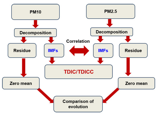
Figure 2. Framework on the multiscale correlation analysis between $PM10$ and $PM2.5$.

4. Results and Discussion

4.1. Multiscale Decomposition

As the first step in the multiscale analysis of the air pollutant concentrations of $PM10$ and $PM2.5$, both time series were decomposed using ICEEMDAN with a noise parameter of 0.1 and an ensemble number of 300 (number of realizations). To validate the correctness of the ICEEMDAN decomposition, the Index of Orthogonality (IO) of the modes was computed as per the recommendations given by Huang et al. [35] with $IO={\sum }_{t=0}^T\left({\sum }_{j=1}^{n+1}{\sum }_{k=1}^{n+1}\frac{C_j\left(t\right)C_k\left(t\right)}{X^2\left(t\right)}\right)$; C represents the oscillatory modes, n is the number of IMFs, X is the signal, and T is the index for the length of the time series. In this study, IO values were $6.37\times {10}^{-4}$ and $5.72\times {10}^{-4}$, respectively, for $PM10$ and $PM2.5$, which are much less than zero, validating the correctness of the ICEEMDAN decomposition. The decomposition resulted in 8 IMFs and a residue, as shown in Figure 3. The first IMF mode showed the fast fluctuations, while the last mode highlighted the slowest fluctuations. Each IMF captured the local variation for a distinct time scale. During the study period, the non-linear trends of both pollutant concentrations decreased. The residues of both pollutants seemed to follow the same temporal behavior. The mean period of each mode was computed using the zero-crossing method [63].

Figure 3. Oscillatory modes of (a) $PM10$ and (b) $PM2.5$ obtained by ICEEMDAN.

Table 1 presents the mean period in days and the percentage of variability explained by different modes. The multiscale decomposition of both time series is accurate as the time scale increases with increasing IMF values. For $PM10$, the variability decreases from IMF1 to IMF6. However, the variability increases for IMF and IMF8, i.e., for the semester and annual scales. In the case of $PM2.5$, there is no significant trend observed over several time scales. However, there is a high variability for the semester scale (IM7). The behavior of both pollutants at the semester scale can be explained by the seasonal cycle of African dust, which lasts around six months in the Caribbean area [22,23].

Table 1. Mean period (days) and variability (%) explained for the different modes of the $PM10$ and $PM2.5$ time series.

	$\mathit{P}\mathit{M}10$		$\mathit{P}\mathit{M}2.5$
Modes	Mean Period (Days)	Variability (%)	Mean Period (Days)	Variability (%)
IMF1	3.102	22.698	2.866	17.265
IMF2	6.403	18.962	6.844	14.432
IMF3	12.303	14.040	13.353	15.795
IMF4	23.297	7.331	24.333	6.477
IMF5	40.555	6.553	47.608	11.200
IMF6	73.000	3.486	91.250	10.264
IMF	182.500	7.914	219.000	15.535
IMF8	365.000	13.676	365.000	5.451
Residue	1095.000	5.337	1095.000	3.577

4.2. Hilbert Spectral Analysis

The temporal changes in amplitude at each time scale were determined, which can be visualized by plotting the IF trajectories associated with each IMF. In Figure 4, a high degree of intermittency is noted in IMF1 (high-frequency mode), while more continuous spectra are noted in the subsequent low-frequency modes for $PM2.5$. One can easily notice that the contributions of the highest amplitudes are observed at different time instants/spells. In the spectra of IMF2 to 5, the concentration of high amplitudes is highly localized in time, whereas in the IMF6 and IMF of seasonal to intra-seasonal scales, the contribution of high amplitudes is sustained for long and continuous periods. Similar observations can also be made from Figure 5, depicting the time-frequency amplitude (TFA) spectra of different IMFs of $PM10$. Singularities are noted in the spectra between 2006 and 2008 for IMF4 and IMF5.

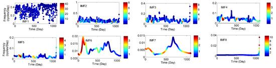
Figure 4. Time-frequency amplitude spectra of IMFs for $PM2.5$.

Figure 5. Time-frequency amplitude spectra of IMFs for $PM10$.

The mean amplitude (MA) and mean frequencies (MF) of different IMFs of $PM10$ and $PM2.5$ are shown in Table 2. At annual cycles, the mean amplitudes are concentrated around 8.7 $\mathsf{\mu }$g/m${}^3$ and 0.98 $\mathsf{\mu }$g/m${}^3$, respectively, for $PM10$ and $PM2.5$. The trends of instantaneous amplitudes (IAs) of $PM10$ and $PM2.5$ at different scales are computed by the Mann–Kendall test [64,65] at the 5% significance level. Except for the IA of IMF4, the trends are of the same nature. For IMF4 (monthly scale), a significantly increasing trend was noticed for the amplitudes of $PM2.5$, while a decreasing trend was noticed for the amplitudes of $PM10$. At the intra-seasonal scales, a significantly increasing trend was noticed in the amplitudes of $PM10$, while the trend was not significant for the amplitudes of $PM2.5$.

Table 2. Mean and trend of instantaneous amplitudes along with the mean frequencies of different IMFs. Z represents the Mann–Kendall value.

	Parameter	IMF1	IMF2	IMF3	IMF4	IMF5	IMF6	IMF	IMF8
	MA	8.690	7.164	6.049	4.587	4.828	3.994	5.320	8.667
$PM10$	Z value of IA	−2.59	−8.06	−4.82	−1.75	−10.78	−15.50	15.61	28.61
	MF	0.305	0.155	0.077	0.043	0.024	0.013	0.005	0.003
	MA	1.609	1.459	1.511	0.999	1.302	1.372	1.645	0.983
$PM2.5$	Z value of IA	−12.43	−4.99	−4.76	4.36	−3.13	−23.03	0.38	49.05
	MF	0.324	0.145	0.072	0.041	0.021	0.011	0.005	0.002

From the marginal spectra shown in Figure 6, the maximum amplitudes were 369.48 $\mathsf{\mu }$g/m${}^3$ and 48.13 $\mathsf{\mu }$g/m${}^3$, respectively, for $PM10$ and $PM2.5$. From the marginal spectrum, two dominant peaks around the weekly scale are evident in both $PM$ types. In addition to this, there are at least two more dominant peaks, ∼3 d are noted in the spectra of $PM2.5$. Moreover, the spectrum of $PM2.5$ is more regular and stable. Multiple visible prominent peaks exist in the spectra of $PM2.5$, which fall in daily to monthly time scales, indicating the frequent disposal of pollutants. This can be due to the fact that $PM2.5$ is more representative of anthropogenic activity [66,67]. In general, the typical behavior of frequent pollutant disposal to the atmosphere is very much evident from the spikes of the marginal spectra of both $PM$ series.

Figure 6. Marginal Hilbert spectrum of (a) $PM10$ and (b) $PM2.5$.

4.3. TDIC Analysis

From the TDIC plots in Figure 7, it can be seen that there are rich dynamics in the correlation between $PM2.5$ and $PM10$ at all timescales of less than a month. The maximum strength was deciphered at quarterly (IMF6 = ∼2.5 to 3 months) and annual scales (IMF8 = 1 year), and the correlation was found to be strongly positive. This behavior may be due to the seasonality of African dust. Numerous studies have shown that there is a low dust season in the Caribbean area from October to April and a high dust season from May to September [22,23,24,25,68]. Euphrasie-Clotilde et al. [23] highlighted that the peak of the high dust season is from June to August, i.e., a 3-month period. During a sand haze, $PM2.5$ and $PM10$ concentrations increase significantly [33,34].

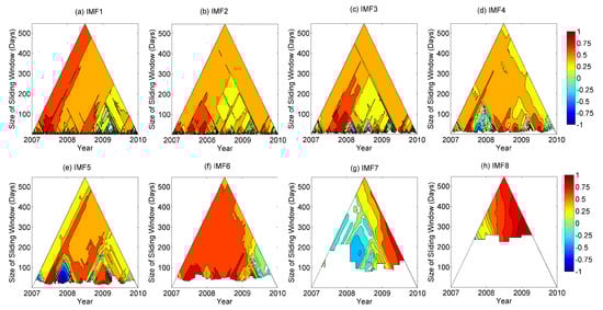
Figure 7. TDIC plots of $PM10$ vs. $PM2.5$ at different scales. The white spaces imply that the correlation is not significant at the 5% level.

However, there is a switchover from positive to negative in most of the time scales, over the time period. A strong negative correlation was noticed at an intra-annual time scale of 1.5 months (IMF5) in the period of the highest pollutant concentrations (in 2007). After dust outbreaks, i.e., high $PM2.5$ and $PM10$ concentrations, the rainfall helps restore the particulate matter atmospheric balance [69] by the wet scavenging process [70,71]. Since $PM10$ particles are larger than $PM2.5$, they are more easily trapped by water droplets. Thus, the wet scavenging process is less effective for $PM2.5$[72]. Consequently, the $PM2.5$ remains suspended in the atmosphere longer than $PM10$, which may explain this strong negative correlation. At a periodic scale of 6 months (IMF), the correlation was mostly negative, which may be due to the rainfall cycle, which is crucial in influencing the $PM2.5$–$PM10$ relationship. In Puerto Rico, the rainy season occurs from May to November [73] during the hurricane season.

4.4. TDICC Analysis

As the next phase of our analysis, we computed time-lagged correlations between $PM10$ and $PM2.5$ by invoking the TDICC analysis. We captured lagged information for up to a week for each mode (time scale), which provided some interesting observations in terms of correlation patterns at different scales.

At the high-frequency IMF (∼3 d), the TDIC plot in Figure 8 shows a positive association, but from lag 1 onward, there is a negative correlation. Moreover, unlike the TDIC plot at lag 0, more insignificant spaces are present in the correlation patterns when considering the antecedent pollutant information.

Figure 8. TDICC analysis of high-frequency (IMF1). The white spaces imply that the correlation is not significant at the 5% level.

Upon considering the TDICC analysis of IMF2 in Figure 9, the correlation is positive at lag 1, but between lag 2 to lag 5, the correlations are primarily negative. Here, in lag 3 and lag 4, the correlation is in the long range, over the complete time spell and time window, indicating a stable correlation pattern, which makes it significant for the prediction of IMF2. Thus, $IMF2$ can be computed as $IMF2\left(t\right)=f\left(IMF2\right(t-3),IMF2(t-4\left)\right)$.

Figure 9. TDICC analysis of IMFs at the weekly time scale (IMF2). The white spaces imply that the correlation is not significant at the 5% level.

Regarding IMF3 in Figure 10, for the first three lags, the correlation is primarily positive, while in the remaining lags, we can see that the correlation is negative with more stable patterns for lag 6 and lag 7. The TDICC analysis of IMF4 in Figure 11 shows a stable positive pattern up to lag 3; thereafter, the correlation is negatively dominated and the stable pattern is noticed at lag 6. In general, the correlation patterns were similar for IMF2, IMF3, and IMF4. These results show a behavioral uniformity between $PM10$ and $PM2.5$ for time scales between ∼1 and 3 weeks.

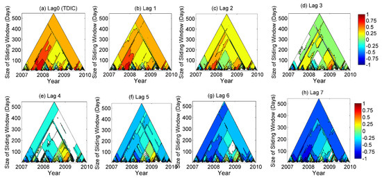
Figure 10. TDICC analysis of IMFs at the ∼2-week time scale (IMF3). The white spaces imply that the correlation is not significant at the 5% level.

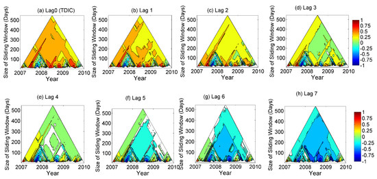
Figure 11. TDICC analysis of IMFs at the ∼3-week time scale (IMF4). The white spaces imply that the correlation is not significant at the 5% level.

For the TDICC analysis of IMF5, which has a periodicity of ∼1.5 months (as seen in Figure 12), the correlation pattern is similar at all lags, except for the magnitude of correlations. It is evident that during the colder period leading up to the peak (2007–2008), the correlation is strongly negative at smaller time windows. In general, the correlation is weakly positive over long ranges at all time lags. For the quarterly scale in Figure 13 (IMF6), the correlation is much stronger and more stable. For the 3-month, 6-month (see Figure 14), and annual cycle IMFs (see Figure 15), the correlation patterns are very strongly positive and long-range. Thus, lag 1 may be sufficient for modeling IMF5 to IMF8.

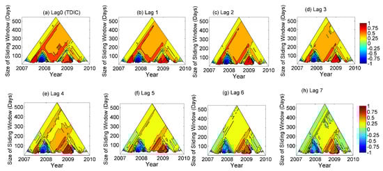
Figure 12. TDICC analysis of IMFs at the intra-annual time scale of ∼1.5 months (IMF5). The white spaces imply that the correlation is not significant at the 5% level.

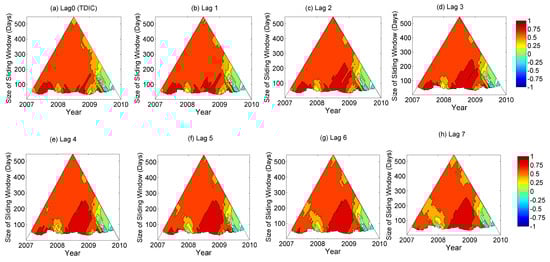
Figure 13. TDICC analysis of IMFs at the quarterly time scale (IMF6). The white spaces imply that the correlation is not significant at the 5% level.

Figure 14. TDICC analysis of IMFs at the semester time scale (IMF). The white spaces imply that the correlation is not significant at the 5% level.

Figure 15. TDICC analysis of IMFs at the annual time scale (IMF8). The white spaces imply that the correlation is not significant at the 5% level.

Moreover, we determined the zero-mean series of residue components and plotted them in Figure 16. The residue components show a very strong correlation of 0.996. Moreover, the zero-crossing of these modes occurs at nearly the same time instant (∼after 70 days, in 2008) and the modes show a similar pattern of evolution.

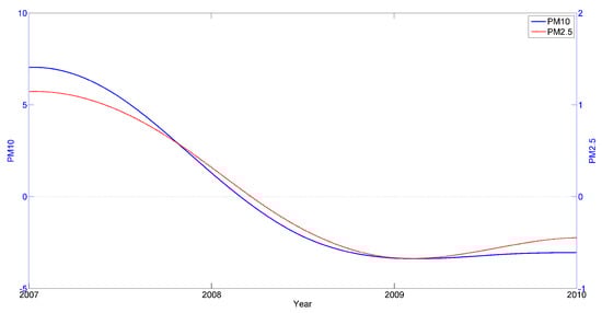
Figure 16. Temporal evolution of low-frequency components of $PM10$ and $PM2.5$.

A large number of machine learning, deep learning, and hybrid variants have been developed to model air pollutants either in a time series or a cause–effect approach [74,75,76,77]. The multiscale correlation analysis performed in this study will be helpful in identifying the most relevant predictors for developing hybrid decomposition–machine learning or deep learning models for predicting air pollutants. Frameworks for such models have already been reported in literature studies for predicting different kinds of geophysical series [49,50,78]. Therefore, this study has great potential to improve the forecasts of air quality parameters.

5. Conclusions

The Caribbean basin has some of the highest incidences of asthma on the planet due to dust outbreaks. Therefore, it is crucial to have accurate information on the behavior of particulate pollutants in order to model and predict them.

HSA was used in this study to identify two dominant peaks around the weekly scale for $PM2.5$ and $PM10$. The concentrations of high amplitudes persisted for long and continuous time periods at seasonal to intra-seasonal scales, while the trends of spectral amplitudes were found to be similar for both $PM$ types, except for monthly and intra-seasonal scales of six months.

The relationships between $PM2.5$ and $PM10$ were studied using a multiscale approach. A novel ICEEMDAN-TDICC coupled framework is proposed to investigate the association between the two pollutants. For the time scales of less than a month, the TDIC analysis showed rich dynamics in the $PM2.5$–$PM10$ correlation due to local and mesoscale sources. For larger time scales (quarterly and annual scales), the correlation was strongly positive due to the dust haze from African deserts. This large-scale source will significantly increase $PM2.5$–$PM10$ concentrations. Consequently, the TDICC analysis highlighted that the $PM2.5$–$PM10$ relationship is stable on a quarterly scale and a lag 1 IMF of $PM2.5$ is enough to model $PM10$. These results show that it will be easier to model $PM10$ from $PM2.5$ during the passage of sand mists because these large-scale events will homogenize the behaviors of particulate pollutants in the atmosphere.

To summarize, we investigated the association between $PM2.5$ and $PM10$ using a multiscale approach. The nature and strength of the association between the two variables were found to be dynamic over different timescales and time spans. However, the reasons behind these transitions were not explored in the present study. Furthermore, various local meteorological factors and large-scale climatic oscillations govern the behavior of $PM2.5$ and $PM10$. Exploring such teleconnections within a multiscale framework may help in understanding the mutual association between $PM2.5$ and $PM10$. Therefore, the findings of the study should be extended to improve predictability efforts.

References

- Tian, G.; Qiao, Z.; Xu, X. Characteristics of particulate matter (PM10) and its relationship with meteorological factors during 2001–2012 in Beijing. Environ. Pollut. 2014, 192, 266–274. [Google Scholar] [CrossRef] [PubMed]
- Choobari, O.A.; Zawar-Reza, P.; Sturman, A. The global distribution of mineral dust and its impacts on the climate system: A review. Atmos. Res. 2014, 138, 152–165. [Google Scholar] [CrossRef]
- Plocoste, T.; Calif, R. Is there a causal relationship between Particulate Matter (PM10) and air Temperature data? An analysis based on the Liang-Kleeman information transfer theory. Atmos. Pollut. Res. 2021, 12, 101177. [Google Scholar] [CrossRef]
- Anderson, J.O.; Thundiyil, J.G.; Stolbach, A. Clearing the air: A review of the effects of particulate matter air pollution on human health. J. Med. Toxicol. 2012, 8, 166–175. [Google Scholar] [CrossRef] [PubMed]
- Hamanaka, R.B.; Mutlu, G.M. Particulate matter air pollution: Effects on the cardiovascular system. Front. Endocrinol. 2018, 9, 680. [Google Scholar] [CrossRef]
- Urrutia-Pereira, M.; Rizzo, L.V.; Staffeld, P.L.; Chong-Neto, H.J.; Viegi, G.; Solé, D. Dust from the Sahara to the American Continent: Health impacts: Dust from Sahara. Allergol. Immunopathol. 2021, 49, 187–194. [Google Scholar] [CrossRef]
- Plocoste, T.; Calif, R.; Euphrasie-Clotilde, L.; Brute, F.N. Investigation of local correlations between particulate matter (PM10) and air temperature in the Caribbean basin using Ensemble Empirical Mode Decomposition. Atmos. Pollut. Res. 2020, 11, 1692–1704. [Google Scholar] [CrossRef]
- Plocoste, T. Multiscale analysis of the dynamic relationship between particulate matter (PM10) and meteorological parameters using CEEMDAN: A focus on “Godzilla” African dust event. Atmos. Pollut. Res. 2022, 13, 101252. [Google Scholar] [CrossRef]
- Bell, M.L.; Dominici, F.; Ebisu, K.; Zeger, S.L.; Samet, J.M. Spatial and temporal variation in PM2.5 chemical composition in the United States for health effects studies. Environ. Health Perspect. 2007, 115, 989–995. [Google Scholar] [CrossRef]
- Polichetti, G.; Cocco, S.; Spinali, A.; Trimarco, V.; Nunziata, A. Effects of particulate matter (PM10, PM2.5 and PM1) on the cardiovascular system. Toxicology 2009, 261, 1–8. [Google Scholar] [CrossRef]
- Lu, F.; Xu, D.; Cheng, Y.; Dong, S.; Guo, C.; Jiang, X.; Zheng, X. Systematic review and meta-analysis of the adverse health effects of ambient PM2.5 and PM10 pollution in the Chinese population. Environ. Res. 2015, 136, 196–204. [Google Scholar] [CrossRef] [PubMed]
- Orellano, P.; Reynoso, J.; Quaranta, N.; Bardach, A.; Ciapponi, A. Short-term exposure to particulate matter (PM10 and PM2.5), nitrogen dioxide (NO2), and ozone (O3) and all-cause and cause-specific mortality: Systematic review and meta-analysis. Environ. Int. 2020, 142, 105876. [Google Scholar] [CrossRef] [PubMed]
- Plocoste, T.; Calif, R.; Jacoby-Koaly, S. Temporal multiscaling characteristics of particulate matter PM10 and ground-level ozone O3 concentrations in Caribbean region. Atmos. Environ. 2017, 169, 22–35. [Google Scholar] [CrossRef]
- Zhang, C.; Ni, Z.; Ni, L. Multifractal detrended cross-correlation analysis between PM2.5 and meteorological factors. Phys. Stat. Mech. Its Appl. 2015, 438, 114–123. [Google Scholar] [CrossRef]
- Wang, Q. Multifractal characterization of air polluted time series in China. Phys. Stat. Mech. Its Appl. 2019, 514, 167–180. [Google Scholar] [CrossRef]
- Plocoste, T.; Carmona-Cabezas, R.; Jiménez-Hornero, F.J.; de Ravé, E.G.; Calif, R. Multifractal characterisation of particulate matter (PM10) time series in the Caribbean basin using visibility graphs. Atmos. Pollut. Res. 2021, 12, 100–110. [Google Scholar] [CrossRef]
- Li, L.; Qian, J.; Ou, C.Q.; Zhou, Y.X.; Guo, C.; Guo, Y. Spatial and temporal analysis of Air Pollution Index and its timescale-dependent relationship with meteorological factors in Guangzhou, China, 2001–2011. Environ. Pollut. 2014, 190, 75–81. [Google Scholar] [CrossRef]
- Fu, H.; Zhang, Y.; Liao, C.; Mao, L.; Wang, Z.; Hong, N. Investigating PM2.5 responses to other air pollutants and meteorological factors across multiple temporal scales. Sci. Rep. 2020, 10, 1–10. [Google Scholar] [CrossRef]
- Filonchyk, M.; Yan, H.; Yang, S.; Hurynovich, V. A study of PM2.5 and PM10 concentrations in the atmosphere of large cities in Gansu Province, China, in summer period. J. Earth Syst. Sci. 2016, 125, 1175–1187. [Google Scholar] [CrossRef]
- Munir, S.; Habeebullah, T.M.; Mohammed, A.M.; Morsy, E.A.; Rehan, M.; Ali, K. Analysing PM2.5 and its association with PM10 and meteorology in the arid climate of Makkah, Saudi Arabia. Aerosol Air Qual. Res. 2017, 17, 453–464. [Google Scholar] [CrossRef]
- Plocoste, T.; Dorville, J.F.; Monjoly, S.; Jacoby-Koaly, S.; André, M. Assessment of Nitrogen Oxides and Ground-Level Ozone behavior in a dense air quality station network: Case study in the Lesser Antilles Arc. J. Air Waste Manag. Assoc. 2018, 68, 1278–1300. [Google Scholar] [CrossRef] [PubMed]
- Prospero, J.M.; Collard, F.X.; Molinié, J.; Jeannot, A. Characterizing the annual cycle of African dust transport to the Caribbean Basin and South America and its impact on the environment and air quality. Glob. Biogeochem. Cycles 2014, 28, 757–773. [Google Scholar] [CrossRef]
- Euphrasie-Clotilde, L.; Plocoste, T.; Feuillard, T.; Velasco-Merino, C.; Mateos, D.; Toledano, C.; Brute, F.N.; Bassette, C.; Gobinddass, M. Assessment of a new detection threshold for PM10 concentrations linked to African dust events in the Caribbean Basin. Atmos. Environ. 2020, 224, 117354. [Google Scholar] [CrossRef]
- Plocoste, T.; Calif, R.; Euphrasie-Clotilde, L.; Brute, F. The statistical behavior of PM10 events over guadeloupean archipelago: Stationarity, modelling and extreme events. Atmos. Res. 2020, 241, 104956. [Google Scholar] [CrossRef]
- Plocoste, T.; Euphrasie-Clotilde, L.; Calif, R.; Brute, F. Quantifying spatio-temporal dynamics of African dust detection threshold for PM10 concentrations in the Caribbean area using multiscale decomposition. Front. Environ. Sci. 2022, 10, 566. [Google Scholar] [CrossRef]
- Alexis, E.; Plocoste, T.; Nuiro, S.P. Analysis of Particulate Matter (PM10) Behavior in the Caribbean Area Using a Coupled SARIMA-GARCH Model. Atmosphere 2022, 13, 862. [Google Scholar] [CrossRef]
- Plocoste, T.; Laventure, S. Forecasting PM10 Concentrations in the Caribbean Area Using Machine Learning Models. Atmosphere 2023, 14, 134. [Google Scholar] [CrossRef]
- Reid, J.S.; Jonsson, H.H.; Maring, H.B.; Smirnov, A.; Savoie, D.L.; Cliff, S.S.; Reid, E.A.; Livingston, J.M.; Meier, M.M.; Dubovik, O.; et al. Comparison of size and morphological measurements of coarse mode dust particles from Africa. J. Geophys. Res. Atmos. 2003, 108, D19. [Google Scholar] [CrossRef]
- Adams, A.M.; Prospero, J.M.; Zhang, C. CALIPSO-derived three-dimensional structure of aerosol over the Atlantic Basin and adjacent continents. J. Clim. 2012, 25, 6862–6879. [Google Scholar] [CrossRef]
- Prospero, J.M.; Delany, A.C.; Delany, A.C.; Carlson, T.N. The Discovery of African Dust Transport to the Western Hemisphere and the Saharan Air Layer: A History. Bull. Am. Meteorol. Soc. 2021, 102, E1239–E1260. [Google Scholar] [CrossRef]
- Stull, R.B. An Introduction to Boundary Layer Meteorology; Springer Science & Business Media: Berlin/Heidelberg, Germany, 2012; Volume 13, p. 666. [Google Scholar]
- Cadelis, G.; Tourres, R.; Molinie, J. Short-term effects of the particulate pollutants contained in Saharan dust on the visits of children to the emergency department due to asthmatic conditions in Guadeloupe (French Archipelago of the Caribbean). PLoS ONE 2014, 9, e91136. [Google Scholar] [CrossRef] [PubMed]
- Euphrasie-Clotilde, L.; Plocoste, T.; Brute, F.N. Particle Size Analysis of African Dust Haze over the Last 20 Years: A Focus on the Extreme Event of June 2020. Atmosphere 2021, 12, 502. [Google Scholar] [CrossRef]
- Duarte, A.L.; Schneider, I.L.; Artaxo, P.; Oliveira, M.L. Spatiotemporal assessment of particulate matter (PM10 and PM2.5) and ozone in a Caribbean urban coastal city. Geosci. Front. 2022, 13, 101168. [Google Scholar] [CrossRef]
- Huang, N.E.; Shen, Z.; Long, S.R.; Wu, M.C.; Shih, H.H.; Zheng, Q.; Yen, N.C.; Tung, C.C.; Liu, H.H. The empirical mode decomposition and the Hilbert spectrum for nonlinear and non-stationary time series analysis. In Proceedings of the Royal Society of London A: Mathematical, Physical and Engineering Sciences; The Royal Society: London, UK, 1998; Volume 454, pp. 903–995. [Google Scholar]
- Huang, N.E.; Shen, Z.; Long, S.R. A new view of nonlinear water waves: The Hilbert spectrum. Annu. Rev. Fluid Mech. 1999, 31, 417–457. [Google Scholar] [CrossRef]
- Flandrin, P.; Goncalves, P. Empirical mode decompositions as data-driven wavelet-like expansions. Int. J. Wavelets Multiresolut. Inf. Process. 2004, 2, 477–496. [Google Scholar] [CrossRef]
- Yeh, J.R.; Shieh, J.S.; Huang, N.E. Complementary ensemble empirical mode decomposition: A novel noise enhanced data analysis method. Adv. Adapt. Data Anal. 2010, 2, 135–156. [Google Scholar] [CrossRef]
- Cao, J.; Li, Z.; Li, J. Financial time series forecasting model based on CEEMDAN and LSTM. Phys. Stat. Mech. Its Appl. 2019, 519, 127–139. [Google Scholar] [CrossRef]
- Wu, Z.; Huang, N.E. Ensemble empirical mode decomposition: A noise-assisted data analysis method. Adv. Adapt. Data Anal. 2009, 1, 1–41. [Google Scholar] [CrossRef]
- Luukko, P.J.; Helske, J.; Räsänen, E. Introducing libeemd: A program package for performing the ensemble empirical mode decomposition. Comput. Stat. 2016, 31, 545–557. [Google Scholar] [CrossRef]
- Torres, M.E.; Colominas, M.A.; Schlotthauer, G.; Flandrin, P. A complete ensemble empirical mode decomposition with adaptive noise. In Proceedings of the 2011 IEEE International Conference on Acoustics, Speech and SIGNAL processing (ICASSP), Prague, Czech Republic, 22–27 May 2011; IEEE: Piscataway, NJ, USA, 2011; pp. 4144–4147. [Google Scholar]
- Colominas, M.A.; Schlotthauer, G.; Torres, M.E. Improved complete ensemble EMD: A suitable tool for biomedical signal processing. Biomed. Signal Process. Control 2014, 14, 19–29. [Google Scholar] [CrossRef]
- Chen, X.; Wu, Z.; Huang, N.E. The time-dependent intrinsic correlation based on the empirical mode decomposition. Adv. Adapt. Data Anal. 2010, 2, 233–265. [Google Scholar] [CrossRef]
- Plocoste, T.; Calif, R.; Jacoby-Koaly, S. Multi-scale time dependent correlation between synchronous measurements of ground-level ozone and meteorological parameters in the Caribbean Basin. Atmos. Environ. 2019, 211, 234–246. [Google Scholar] [CrossRef]
- Tsai, C.W.; Hsiao, Y.R.; Lin, M.L.; Hsu, Y. Development of a noise-assisted multivariate empirical mode decomposition framework for characterizing PM2.5 air pollution in Taiwan and its relation to hydro-meteorological factors. Environ. Int. 2020, 139, 105669. [Google Scholar] [CrossRef] [PubMed]
- Afanasyev, D.O.; Fedorova, E.A.; Popov, V.U. Fine structure of the price-demand relationship in the electricity market: Multi-scale correlation analysis. Energy Econ. 2015, 51, 215–226. [Google Scholar] [CrossRef]
- Adarsh, S.; Reddy, M.J. Investigating the multiscale variability and teleconnections of extreme temperature over Southern India using the Hilbert–Huang transform. Model. Earth Syst. Environ. 2017, 3, 8. [Google Scholar] [CrossRef]
- Adarsh, S.; Reddy, M.J. Multiscale characterization and prediction of monsoon rainfall in India using Hilbert–Huang transform and time-dependent intrinsic correlation analysis. Meteorol. Atmos. Phys. 2018, 130, 667–688. [Google Scholar] [CrossRef]
- Adarsh, S.; Reddy, M.J. Links Between Global Climate Teleconnections and Indian Monsoon Rainfall. In Climate Change Signals and Response; Springer: Berlin/Heidelberg, Germany, 2019; pp. 61–72. [Google Scholar]
- Adarsh, S.; Priya, K. Multiscale running correlation analysis of water quality datasets of Noyyal River, India, using the Hilbert–Huang Transform. Int. J. Environ. Sci. Technol. 2020, 17, 1251–1270. [Google Scholar] [CrossRef]
- Luo, H.; Astitha, M.; Hogrefe, C.; Mathur, R.; Rao, S.T. Evaluating trends and seasonality in modeled PM2.5 concentrations using empirical mode decomposition. Atmos. Chem. Phys. 2020, 20, 13801–13815. [Google Scholar] [CrossRef]
- Wang, M.; Wu, C.; Zhang, P.; Fan, Z.; Yu, Z. Multiscale Dynamic Correlation Analysis of Wind-PV Power Station Output Based on TDIC. IEEE Access 2020, 8, 200695–200704. [Google Scholar] [CrossRef]
- Peng, Q.; Wen, F.; Gong, X. Time-dependent intrinsic correlation analysis of crude oil and the US dollar based on CEEMDAN. Int. J. Financ. Econ. 2021, 26, 834–848. [Google Scholar] [CrossRef]
- Johny, K.; Pai, M.L.; Adarsh, S. Time-dependent intrinsic cross-correlation approach for multi-scale teleconnection analysis for monthly rainfall of India. Meteorol. Atmos. Phys. 2022, 134, 1–22. [Google Scholar] [CrossRef]
- Johny, K.; Pai, M.L.; Adarsh, S. Investigating the multiscale teleconnections of Madden–Julian oscillation and monthly rainfall using time-dependent intrinsic cross-correlation. Nat. Hazards 2022, 112, 1795–1822. [Google Scholar] [CrossRef]
- Peel, M.C.; Finlayson, B.L.; McMahon, T.A. Updated world map of the Köppen-Geiger climate classification. Hydrol. Earth Syst. Sci. 2007, 11, 1633–1644. [Google Scholar] [CrossRef]
- Tartaglione, C.A.; Smith, S.R.; O’Brien, J.J. ENSO impact on hurricane landfall probabilities for the Caribbean. J. Clim. 2003, 16, 2925–2931. [Google Scholar] [CrossRef]
- Dunion, J.P. Rewriting the climatology of the tropical North Atlantic and Caribbean Sea atmosphere. J. Clim. 2011, 24, 893–908. [Google Scholar] [CrossRef]
- Colominas, M.A.; Schlotthauer, G.; Torres, M.E.; Flandrin, P. Noise-assisted EMD methods in action. Adv. Adapt. Data Anal. 2012, 4, 1250025. [Google Scholar] [CrossRef]
- Liu, T.; Luo, Z.; Huang, J.; Yan, S. A comparative study of four kinds of adaptive decomposition algorithms and their applications. Sensors 2018, 18, 2120. [Google Scholar] [CrossRef]
- Huang, Y.; Schmitt, F.G. Time dependent intrinsic correlation analysis of temperature and dissolved oxygen time series using empirical mode decomposition. J. Mar. Syst. 2014, 130, 90–100. [Google Scholar] [CrossRef]
- Huang, N.E.; Wu, Z.; Long, S.R.; Arnold, K.C.; Chen, X.; Blank, K. On instantaneous frequency. Adv. Adapt. Data Anal. 2009, 1, 177–229. [Google Scholar] [CrossRef]
- Mann, H.B. Nonparametric tests against trend. Econom. J. Econom. Soc. 1945, 245–259. [Google Scholar] [CrossRef]
- Kendall, M.G. Rank Correlation Methods; Oxford University Press: Oxford, UK, 1970. [Google Scholar]
- Querol, X.; Alastuey, A.; Rodriguez, S.; Plana, F.; Mantilla, E.; Ruiz, C.R. Monitoring of PM10 and PM2.5 around primary particulate anthropogenic emission sources. Atmos. Environ. 2001, 35, 845–858. [Google Scholar] [CrossRef]
- Colangeli, C.; Palermi, S.; Bianco, S.; Aruffo, E.; Chiacchiaretta, P.; Di Carlo, P. The Relationship between PM2.5 and PM10 in Central Italy: Application of Machine Learning Model to Segregate Anthropogenic from Natural Sources. Atmosphere 2022, 13, 484. [Google Scholar] [CrossRef]
- Plocoste, T.; Pavón-Domínguez, P. Temporal scaling study of particulate matter (PM10) and solar radiation influences on air temperature in the Caribbean basin using a 3D joint multifractal analysis. Atmos. Environ. 2020, 222, 117115. [Google Scholar] [CrossRef]
- Plocoste, T.; Carmona-Cabezas, R.; Jiménez-Hornero, F.J.; Gutiérrez de Ravé, E. Background PM10 atmosphere: In the seek of a multifractal characterization using complex networks. J. Aerosol Sci. 2021, 155, 105777. [Google Scholar] [CrossRef]
- Plocoste, T.; Carmona-Cabezas, R.; Gutiérrez de Ravé, E.; Jimnez-Hornero, F.J. Wet scavenging process of particulate matter (PM10): A multivariate complex network approach. Atmos. Pollut. Res. 2021, 12, 101095. [Google Scholar] [CrossRef]
- Plocoste, T. Detecting the Causal Nexus between Particulate Matter (PM10) and Rainfall in the Caribbean Area. Atmosphere 2022, 13, 175. [Google Scholar] [CrossRef]
- Liu, Z.; Shen, L.; Yan, C.; Du, J.; Li, Y.; Zhao, H. Analysis of the Influence of Precipitation and Wind on PM2.5 and PM10 in the Atmosphere. Adv. Meteorol. 2020, 2020, 5039613. [Google Scholar] [CrossRef]
- Torres-Valcárcel, A.R. Teleconnections between ENSO and rainfall and drought in Puerto Rico. Int. J. Climatol. 2018, 38, e1190–e1204. [Google Scholar] [CrossRef]
- Lei, T.M.; Siu, S.W.; Monjardino, J.; Mendes, L.; Ferreira, F. Using machine learning methods to forecast air quality: A case study in Macao. Atmosphere 2022, 13, 1412. [Google Scholar] [CrossRef]
- Zaini, N.; Ean, L.W.; Ahmed, A.N.; Abdul Malek, M.; Chow, M.F. PM2.5 forecasting for an urban area based on deep learning and decomposition method. Sci. Rep. 2022, 12, 17565. [Google Scholar] [CrossRef]
- Zhang, B.; Rong, Y.; Yong, R.; Qin, D.; Li, M.; Zou, G.; Pan, J. Deep learning for air pollutant concentration prediction: A review. Atmos. Environ. 2022, 290, 119347. [Google Scholar] [CrossRef]
- Méndez, M.; Merayo, M.G.; Nú nez, M. Machine learning algorithms to forecast air quality: A survey. Artif. Intell. Rev. 2023, 1–36. [Google Scholar] [CrossRef] [PubMed]
- Johny, K.; Pai, M.L.; Adarsh, S. A multivariate EMD-LSTM model aided with Time Dependent Intrinsic Cross-Correlation for monthly rainfall prediction. Appl. Soft Comput. 2022, 123, 108941. [Google Scholar] [CrossRef]
Disclaimer/Publisher’s Note: The statements, opinions and data contained in all publications are solely those of the individual author(s) and contributor(s) and not of MDPI and/or the editor(s). MDPI and/or the editor(s) disclaim responsibility for any injury to people or property resulting from any ideas, methods, instructions or products referred to in the content. |
© 2023 by the authors. Licensee MDPI, Basel, Switzerland. This article is an open access article distributed under the terms and conditions of the Creative Commons Attribution (CC BY) license (https://creativecommons.org/licenses/by/4.0/).