


Study of the Dynamical Relationships between PM2.5 and PM10 in the Caribbean Area Using a Multiscale Framework


Abstract
1. Introduction
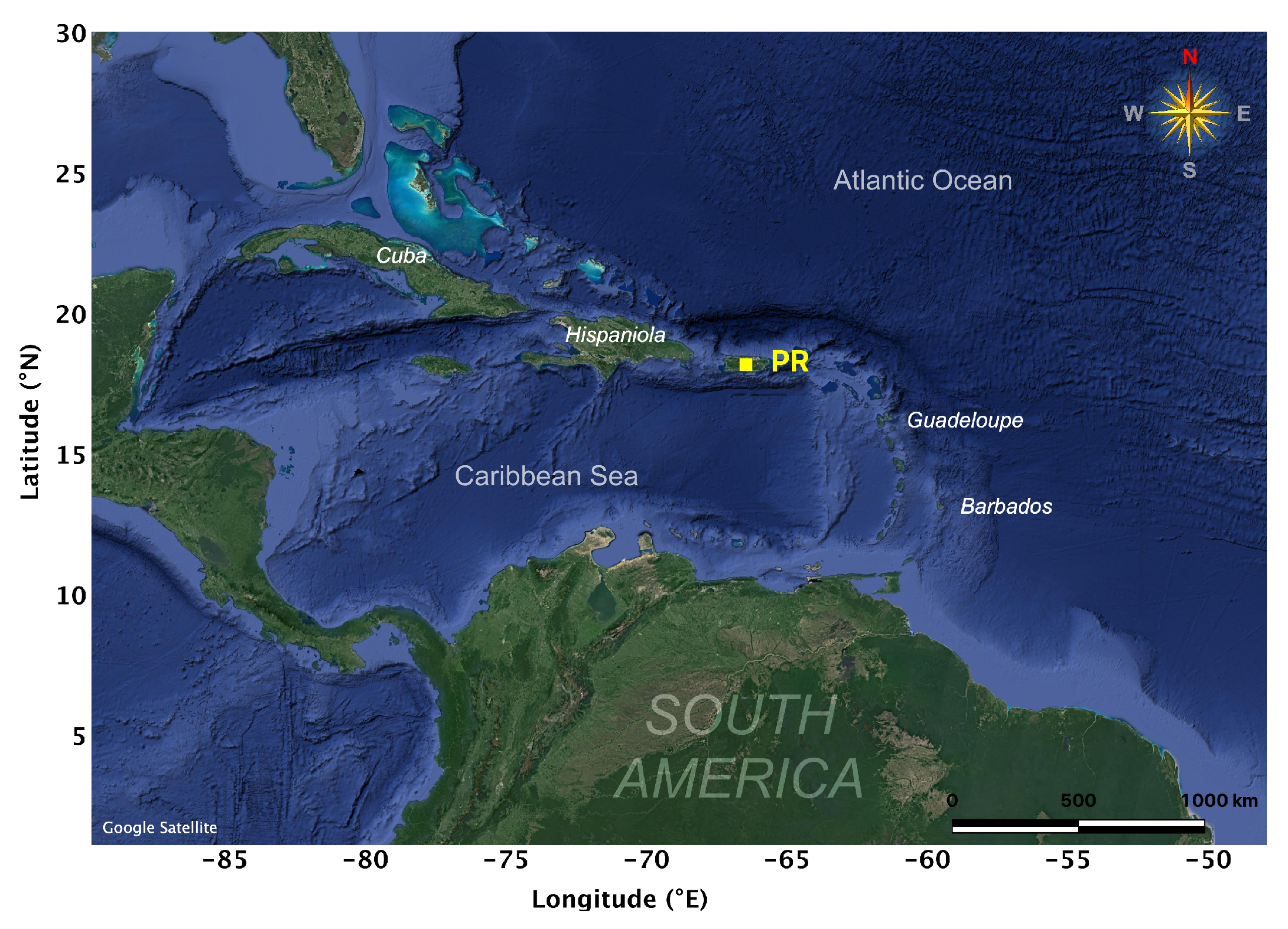
2. Experimental Data
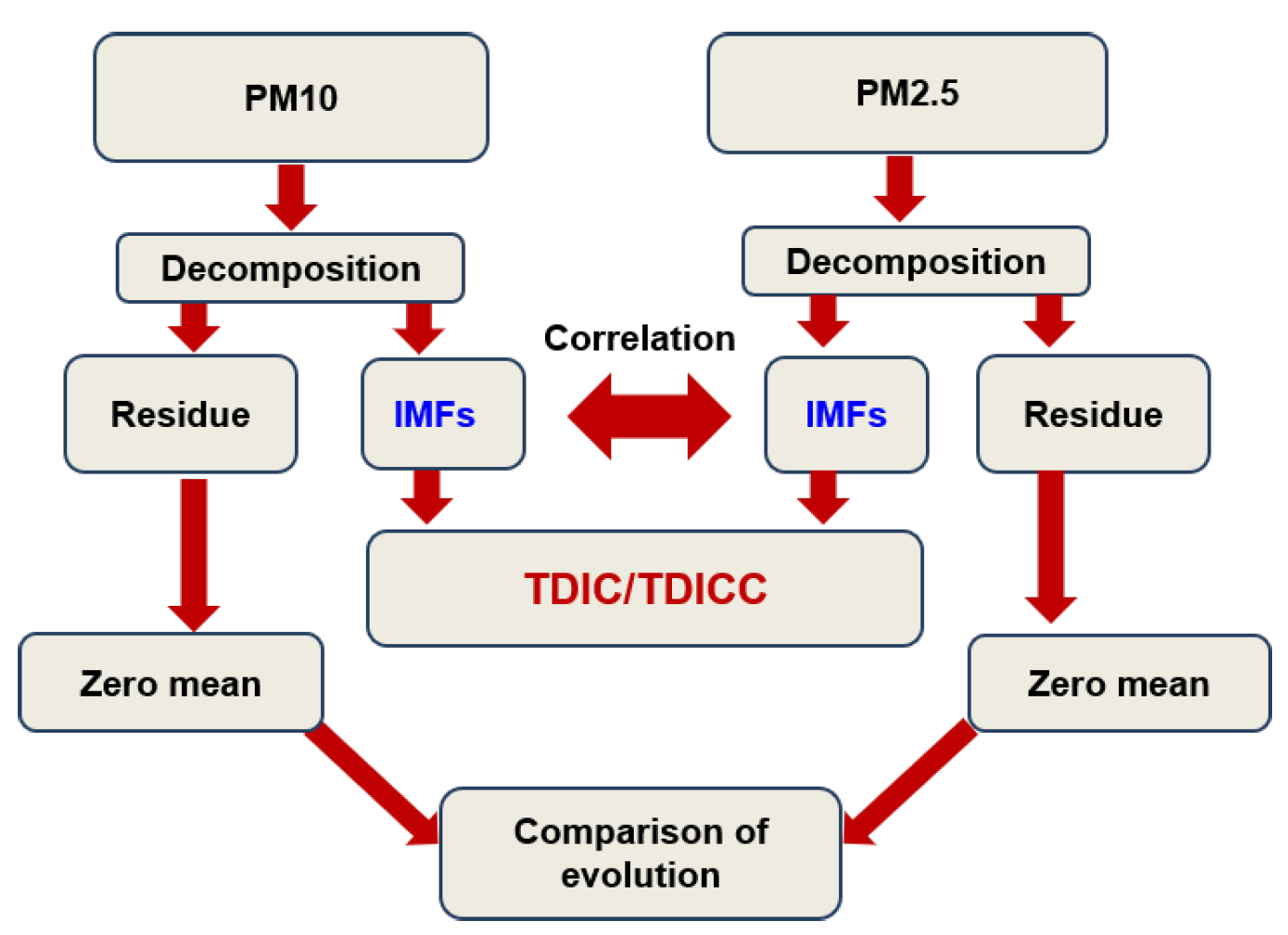
3. Theoretical Framework
3.1. ICEEMDAN
- Compute by EMD the local means of I realizations to obtain the first residue:
- For , compute the first mode:
- Estimate the second residue as the average of local means of the realizations ; the second mode is defined as:
- For , compute the kth residue:
- Calculate the kth mode:
- Repeat step 4 for the next k.
3.2. Hilbert Transform (HT)
3.3. TDIC
- Decompose the two associated time series using ICEEMDAN;
- Determine the HT of each ;
- Find the minimum sliding window size () as the maximum instantaneous period (IP) (reciprocal of IF) between the two IMFs at the current position , i.e.,, where and are IPs;
- Fix the size of the sliding window (SSW) as where n is a multiplication factor usually fixed as unity;
- Find the TDIC of the pair of IMFs as at any , where is the correlation coefficient of two time series;
- Examine the statistical significance of correlation by t-test;
- Repeat steps 4 to 7 in an iterative manner until the boundary of the sliding window exceeds the endpoints of the time series.
3.4. TDICC
- Decompose the two associated time series using ICEEMDAN;
- Apply HT on the IMFs to calculate the IF, then compute the instantaneous periods);
- Fix the minimum sliding window size for the local correlation computation, which is , where and are instantaneous periods of the two IMFs;
- Find the size of the sliding window (SSW) as for a specific IMF of the first signal (say ) and for the corresponding IMF of the second signal, (say ), where n is any positive number, and is usually selected as 1 [62];
- Determine the running correlation between the two modes along with their statistical significance using the TDICC t-test. This can be repeated until the boundary of the sliding window exceeds the endpoints of the time series.
4. Results and Discussion
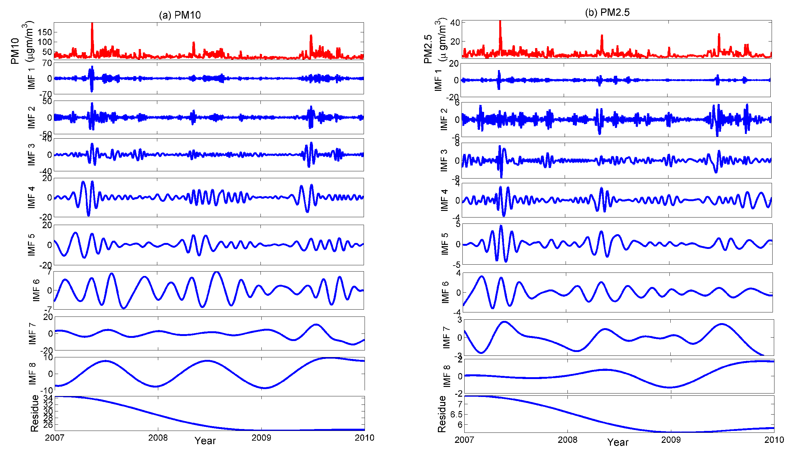
4.1. Multiscale Decomposition
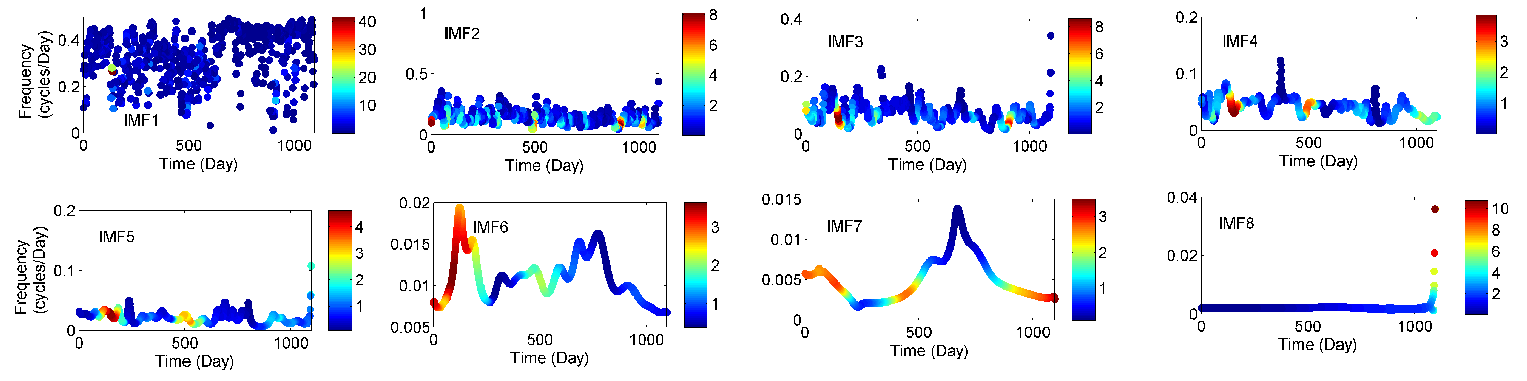
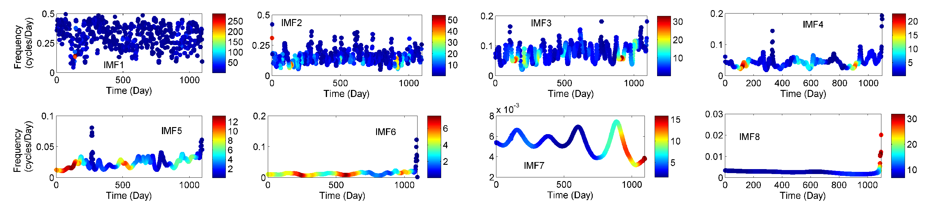
4.2. Hilbert Spectral Analysis
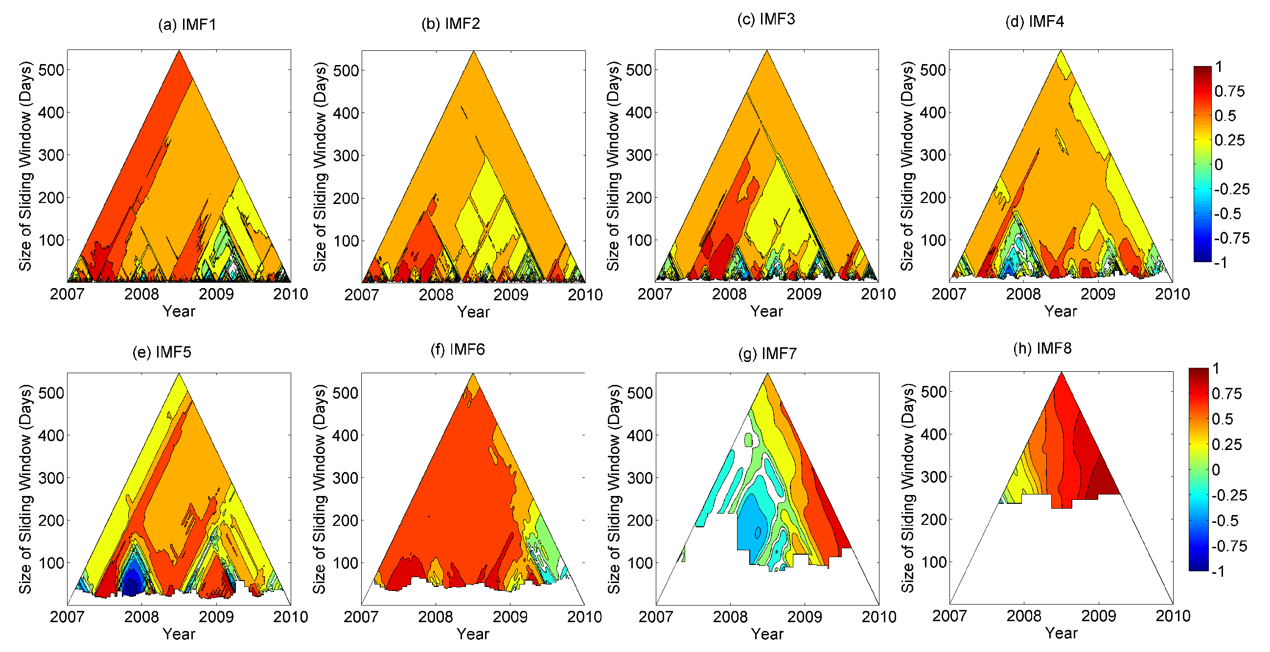
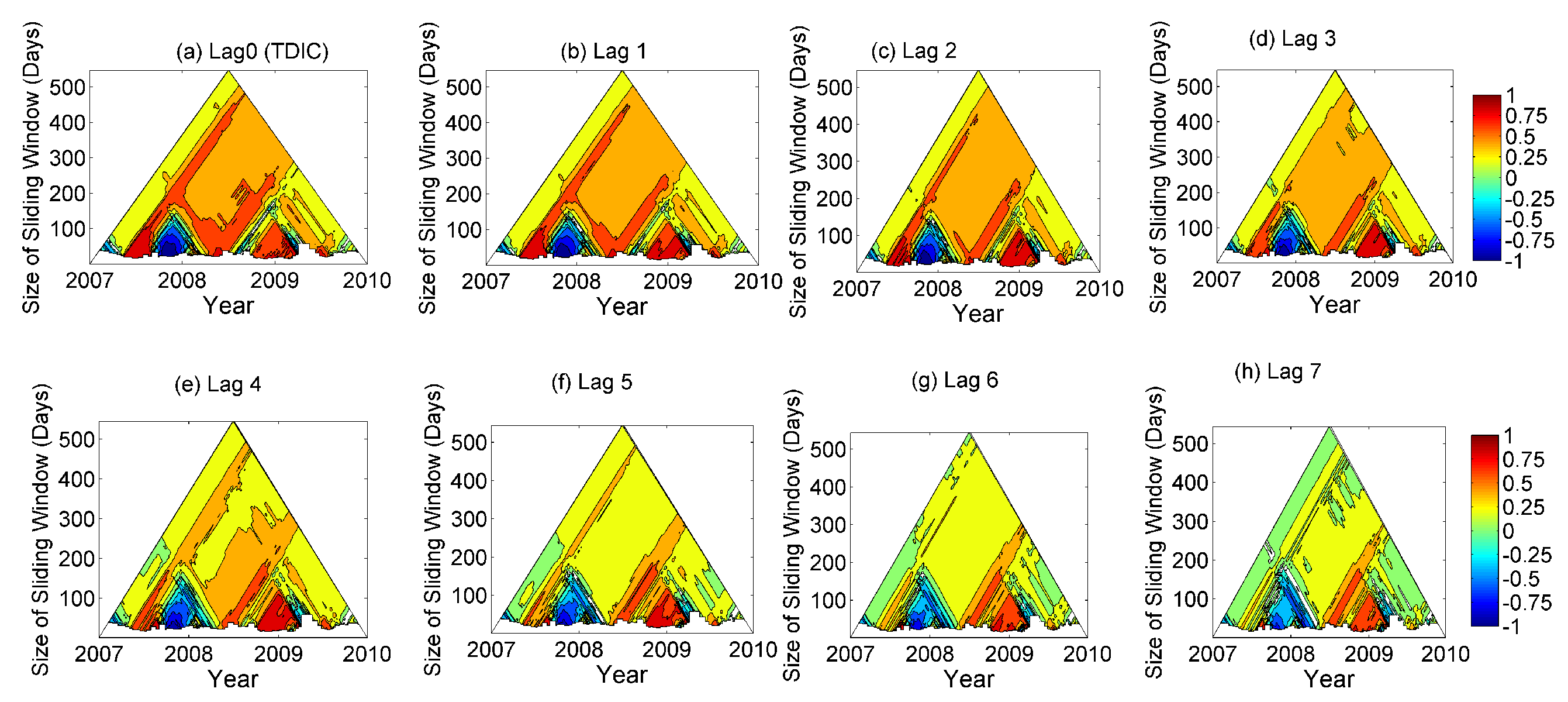
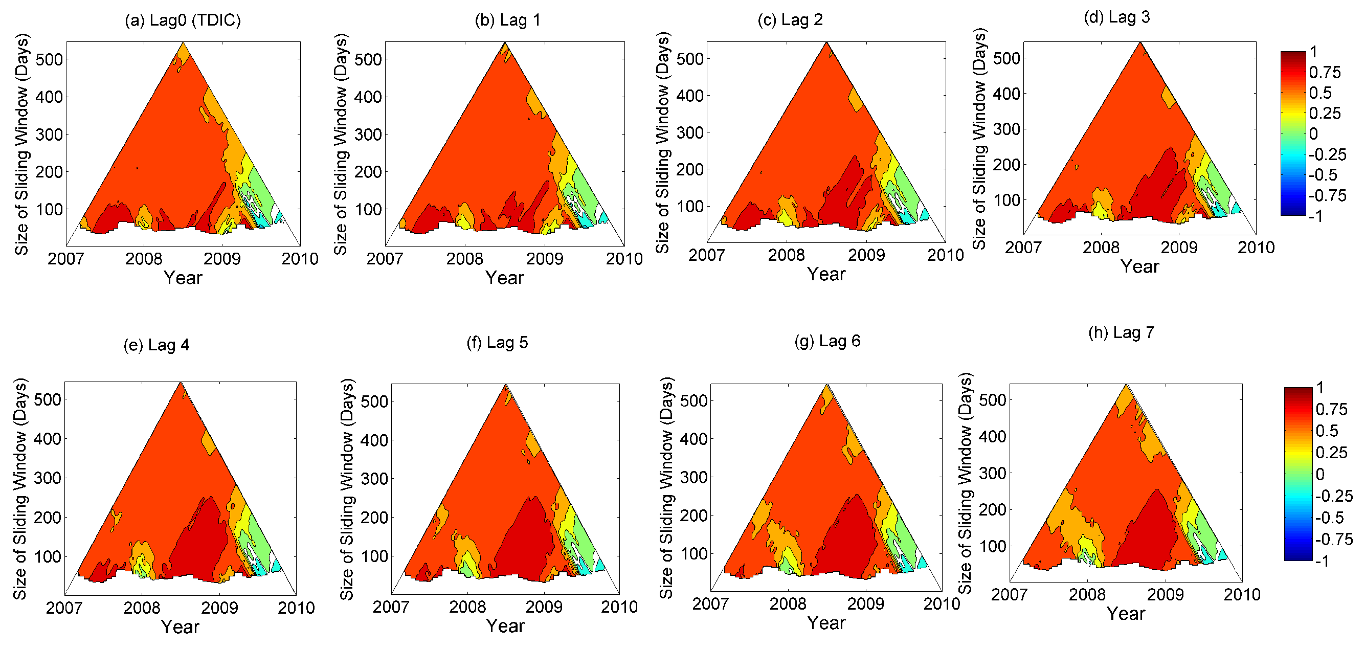
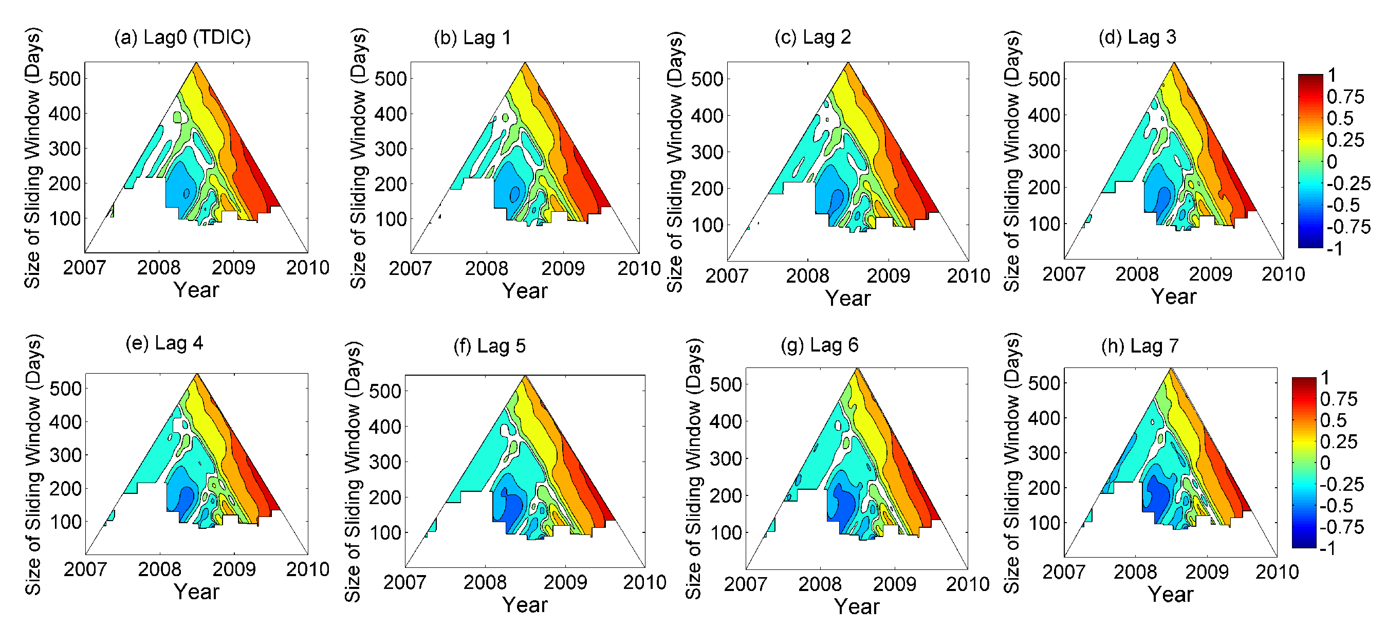
4.3. TDIC Analysis
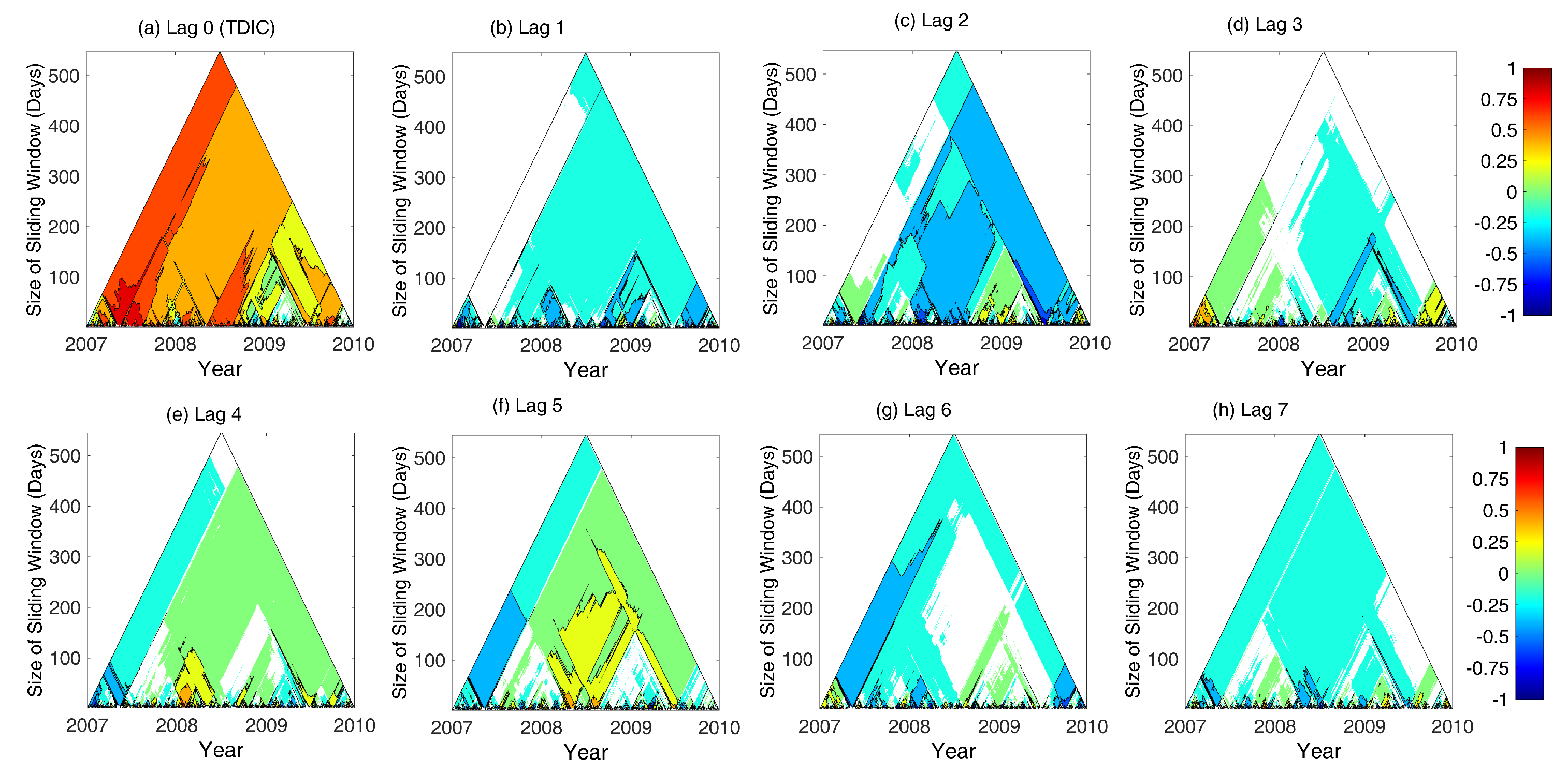
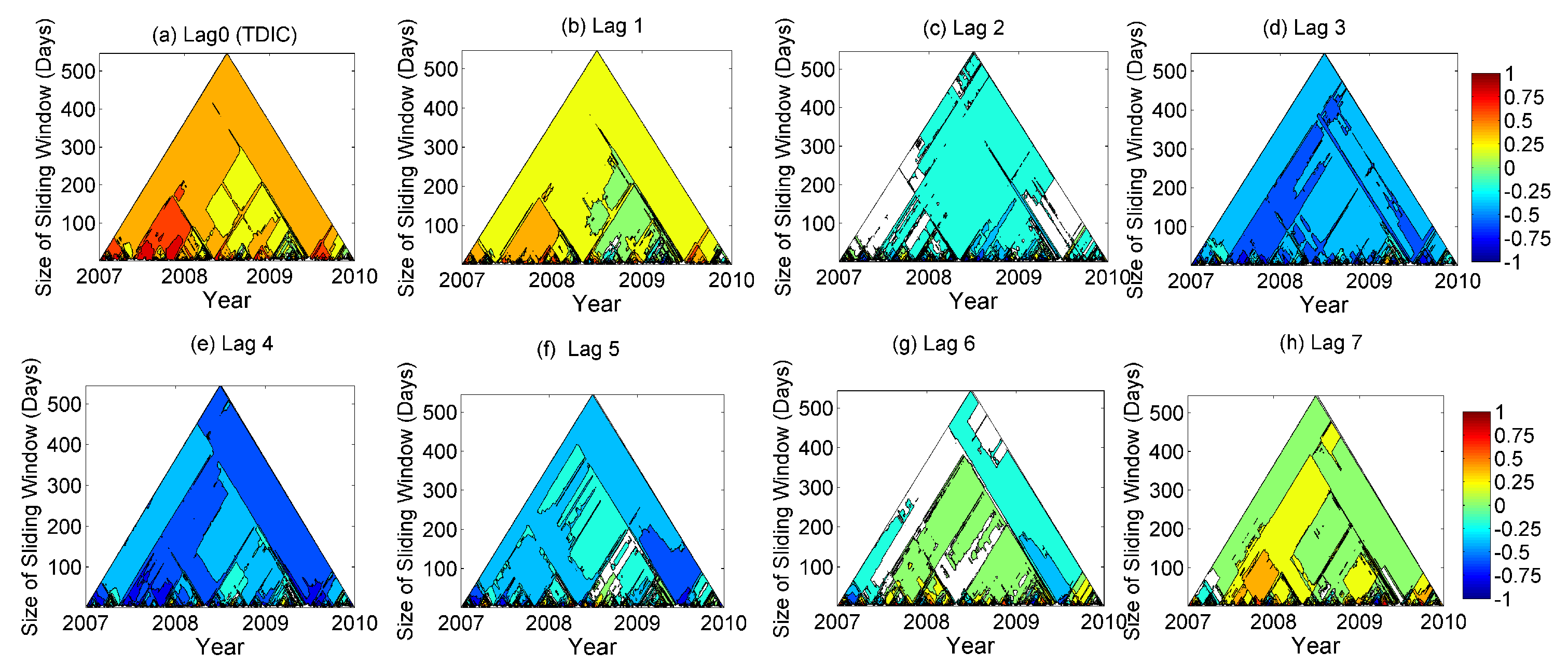
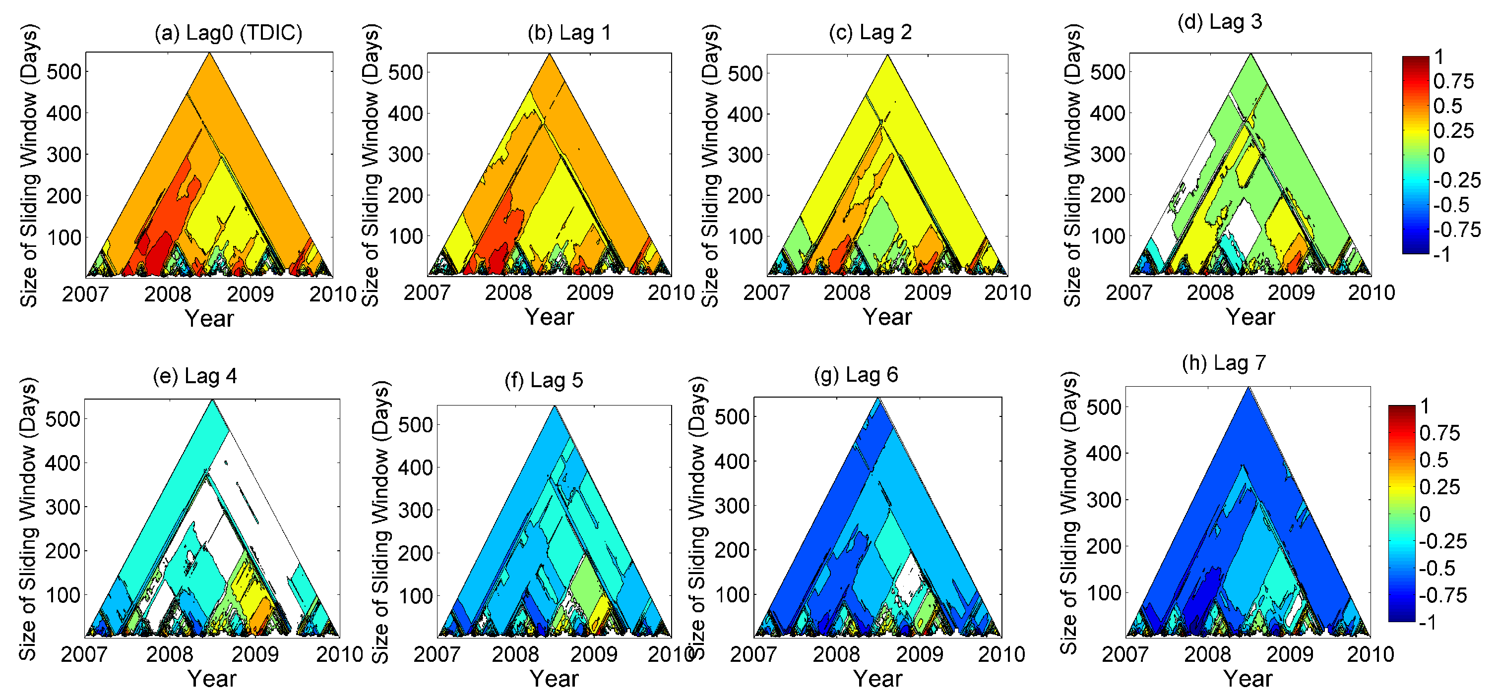
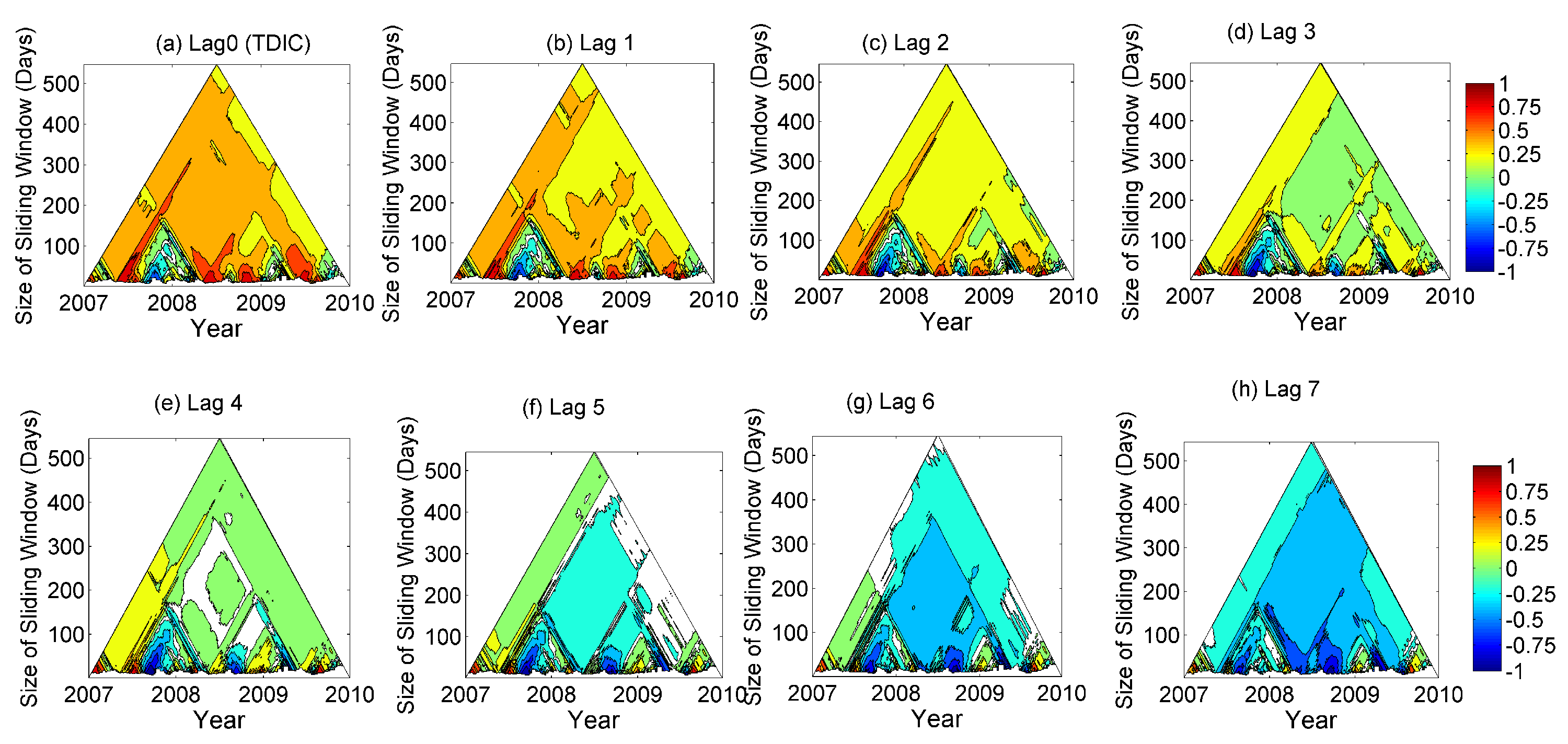
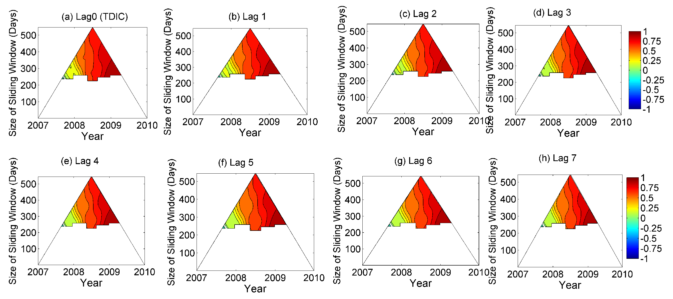
4.4. TDICC Analysis
5. Conclusions
Author Contributions
Funding
Institutional Review Board Statement
Informed Consent Statement
Data Availability Statement
Acknowledgments
Conflicts of Interest
References
- Tian, G.; Qiao, Z.; Xu, X. Characteristics of particulate matter (PM10) and its relationship with meteorological factors during 2001–2012 in Beijing. Environ. Pollut. 2014, 192, 266–274. [Google Scholar] [CrossRef] [PubMed]
- Choobari, O.A.; Zawar-Reza, P.; Sturman, A. The global distribution of mineral dust and its impacts on the climate system: A review. Atmos. Res. 2014, 138, 152–165. [Google Scholar] [CrossRef]
- Plocoste, T.; Calif, R. Is there a causal relationship between Particulate Matter (PM10) and air Temperature data? An analysis based on the Liang-Kleeman information transfer theory. Atmos. Pollut. Res. 2021, 12, 101177. [Google Scholar] [CrossRef]
- Anderson, J.O.; Thundiyil, J.G.; Stolbach, A. Clearing the air: A review of the effects of particulate matter air pollution on human health. J. Med. Toxicol. 2012, 8, 166–175. [Google Scholar] [CrossRef] [PubMed]
- Hamanaka, R.B.; Mutlu, G.M. Particulate matter air pollution: Effects on the cardiovascular system. Front. Endocrinol. 2018, 9, 680. [Google Scholar] [CrossRef]
- Urrutia-Pereira, M.; Rizzo, L.V.; Staffeld, P.L.; Chong-Neto, H.J.; Viegi, G.; Solé, D. Dust from the Sahara to the American Continent: Health impacts: Dust from Sahara. Allergol. Immunopathol. 2021, 49, 187–194. [Google Scholar] [CrossRef]
- Plocoste, T.; Calif, R.; Euphrasie-Clotilde, L.; Brute, F.N. Investigation of local correlations between particulate matter (PM10) and air temperature in the Caribbean basin using Ensemble Empirical Mode Decomposition. Atmos. Pollut. Res. 2020, 11, 1692–1704. [Google Scholar] [CrossRef]
- Plocoste, T. Multiscale analysis of the dynamic relationship between particulate matter (PM10) and meteorological parameters using CEEMDAN: A focus on “Godzilla” African dust event. Atmos. Pollut. Res. 2022, 13, 101252. [Google Scholar] [CrossRef]
- Bell, M.L.; Dominici, F.; Ebisu, K.; Zeger, S.L.; Samet, J.M. Spatial and temporal variation in PM2.5 chemical composition in the United States for health effects studies. Environ. Health Perspect. 2007, 115, 989–995. [Google Scholar] [CrossRef]
- Polichetti, G.; Cocco, S.; Spinali, A.; Trimarco, V.; Nunziata, A. Effects of particulate matter (PM10, PM2.5 and PM1) on the cardiovascular system. Toxicology 2009, 261, 1–8. [Google Scholar] [CrossRef]
- Lu, F.; Xu, D.; Cheng, Y.; Dong, S.; Guo, C.; Jiang, X.; Zheng, X. Systematic review and meta-analysis of the adverse health effects of ambient PM2.5 and PM10 pollution in the Chinese population. Environ. Res. 2015, 136, 196–204. [Google Scholar] [CrossRef] [PubMed]
- Orellano, P.; Reynoso, J.; Quaranta, N.; Bardach, A.; Ciapponi, A. Short-term exposure to particulate matter (PM10 and PM2.5), nitrogen dioxide (NO2), and ozone (O3) and all-cause and cause-specific mortality: Systematic review and meta-analysis. Environ. Int. 2020, 142, 105876. [Google Scholar] [CrossRef] [PubMed]
- Plocoste, T.; Calif, R.; Jacoby-Koaly, S. Temporal multiscaling characteristics of particulate matter PM10 and ground-level ozone O3 concentrations in Caribbean region. Atmos. Environ. 2017, 169, 22–35. [Google Scholar] [CrossRef]
- Zhang, C.; Ni, Z.; Ni, L. Multifractal detrended cross-correlation analysis between PM2.5 and meteorological factors. Phys. Stat. Mech. Its Appl. 2015, 438, 114–123. [Google Scholar] [CrossRef]
- Wang, Q. Multifractal characterization of air polluted time series in China. Phys. Stat. Mech. Its Appl. 2019, 514, 167–180. [Google Scholar] [CrossRef]
- Plocoste, T.; Carmona-Cabezas, R.; Jiménez-Hornero, F.J.; de Ravé, E.G.; Calif, R. Multifractal characterisation of particulate matter (PM10) time series in the Caribbean basin using visibility graphs. Atmos. Pollut. Res. 2021, 12, 100–110. [Google Scholar] [CrossRef]
- Li, L.; Qian, J.; Ou, C.Q.; Zhou, Y.X.; Guo, C.; Guo, Y. Spatial and temporal analysis of Air Pollution Index and its timescale-dependent relationship with meteorological factors in Guangzhou, China, 2001–2011. Environ. Pollut. 2014, 190, 75–81. [Google Scholar] [CrossRef]
- Fu, H.; Zhang, Y.; Liao, C.; Mao, L.; Wang, Z.; Hong, N. Investigating PM2.5 responses to other air pollutants and meteorological factors across multiple temporal scales. Sci. Rep. 2020, 10, 1–10. [Google Scholar] [CrossRef]
- Filonchyk, M.; Yan, H.; Yang, S.; Hurynovich, V. A study of PM2.5 and PM10 concentrations in the atmosphere of large cities in Gansu Province, China, in summer period. J. Earth Syst. Sci. 2016, 125, 1175–1187. [Google Scholar] [CrossRef]
- Munir, S.; Habeebullah, T.M.; Mohammed, A.M.; Morsy, E.A.; Rehan, M.; Ali, K. Analysing PM2.5 and its association with PM10 and meteorology in the arid climate of Makkah, Saudi Arabia. Aerosol Air Qual. Res. 2017, 17, 453–464. [Google Scholar] [CrossRef]
- Plocoste, T.; Dorville, J.F.; Monjoly, S.; Jacoby-Koaly, S.; André, M. Assessment of Nitrogen Oxides and Ground-Level Ozone behavior in a dense air quality station network: Case study in the Lesser Antilles Arc. J. Air Waste Manag. Assoc. 2018, 68, 1278–1300. [Google Scholar] [CrossRef] [PubMed]
- Prospero, J.M.; Collard, F.X.; Molinié, J.; Jeannot, A. Characterizing the annual cycle of African dust transport to the Caribbean Basin and South America and its impact on the environment and air quality. Glob. Biogeochem. Cycles 2014, 28, 757–773. [Google Scholar] [CrossRef]
- Euphrasie-Clotilde, L.; Plocoste, T.; Feuillard, T.; Velasco-Merino, C.; Mateos, D.; Toledano, C.; Brute, F.N.; Bassette, C.; Gobinddass, M. Assessment of a new detection threshold for PM10 concentrations linked to African dust events in the Caribbean Basin. Atmos. Environ. 2020, 224, 117354. [Google Scholar] [CrossRef]
- Plocoste, T.; Calif, R.; Euphrasie-Clotilde, L.; Brute, F. The statistical behavior of PM10 events over guadeloupean archipelago: Stationarity, modelling and extreme events. Atmos. Res. 2020, 241, 104956. [Google Scholar] [CrossRef]
- Plocoste, T.; Euphrasie-Clotilde, L.; Calif, R.; Brute, F. Quantifying spatio-temporal dynamics of African dust detection threshold for PM10 concentrations in the Caribbean area using multiscale decomposition. Front. Environ. Sci. 2022, 10, 566. [Google Scholar] [CrossRef]
- Alexis, E.; Plocoste, T.; Nuiro, S.P. Analysis of Particulate Matter (PM10) Behavior in the Caribbean Area Using a Coupled SARIMA-GARCH Model. Atmosphere 2022, 13, 862. [Google Scholar] [CrossRef]
- Plocoste, T.; Laventure, S. Forecasting PM10 Concentrations in the Caribbean Area Using Machine Learning Models. Atmosphere 2023, 14, 134. [Google Scholar] [CrossRef]
- Reid, J.S.; Jonsson, H.H.; Maring, H.B.; Smirnov, A.; Savoie, D.L.; Cliff, S.S.; Reid, E.A.; Livingston, J.M.; Meier, M.M.; Dubovik, O.; et al. Comparison of size and morphological measurements of coarse mode dust particles from Africa. J. Geophys. Res. Atmos. 2003, 108, D19. [Google Scholar] [CrossRef]
- Adams, A.M.; Prospero, J.M.; Zhang, C. CALIPSO-derived three-dimensional structure of aerosol over the Atlantic Basin and adjacent continents. J. Clim. 2012, 25, 6862–6879. [Google Scholar] [CrossRef]
- Prospero, J.M.; Delany, A.C.; Delany, A.C.; Carlson, T.N. The Discovery of African Dust Transport to the Western Hemisphere and the Saharan Air Layer: A History. Bull. Am. Meteorol. Soc. 2021, 102, E1239–E1260. [Google Scholar] [CrossRef]
- Stull, R.B. An Introduction to Boundary Layer Meteorology; Springer Science & Business Media: Berlin/Heidelberg, Germany, 2012; Volume 13, p. 666. [Google Scholar]
- Cadelis, G.; Tourres, R.; Molinie, J. Short-term effects of the particulate pollutants contained in Saharan dust on the visits of children to the emergency department due to asthmatic conditions in Guadeloupe (French Archipelago of the Caribbean). PLoS ONE 2014, 9, e91136. [Google Scholar] [CrossRef] [PubMed]
- Euphrasie-Clotilde, L.; Plocoste, T.; Brute, F.N. Particle Size Analysis of African Dust Haze over the Last 20 Years: A Focus on the Extreme Event of June 2020. Atmosphere 2021, 12, 502. [Google Scholar] [CrossRef]
- Duarte, A.L.; Schneider, I.L.; Artaxo, P.; Oliveira, M.L. Spatiotemporal assessment of particulate matter (PM10 and PM2.5) and ozone in a Caribbean urban coastal city. Geosci. Front. 2022, 13, 101168. [Google Scholar] [CrossRef]
- Huang, N.E.; Shen, Z.; Long, S.R.; Wu, M.C.; Shih, H.H.; Zheng, Q.; Yen, N.C.; Tung, C.C.; Liu, H.H. The empirical mode decomposition and the Hilbert spectrum for nonlinear and non-stationary time series analysis. In Proceedings of the Royal Society of London A: Mathematical, Physical and Engineering Sciences; The Royal Society: London, UK, 1998; Volume 454, pp. 903–995. [Google Scholar]
- Huang, N.E.; Shen, Z.; Long, S.R. A new view of nonlinear water waves: The Hilbert spectrum. Annu. Rev. Fluid Mech. 1999, 31, 417–457. [Google Scholar] [CrossRef]
- Flandrin, P.; Goncalves, P. Empirical mode decompositions as data-driven wavelet-like expansions. Int. J. Wavelets Multiresolut. Inf. Process. 2004, 2, 477–496. [Google Scholar] [CrossRef]
- Yeh, J.R.; Shieh, J.S.; Huang, N.E. Complementary ensemble empirical mode decomposition: A novel noise enhanced data analysis method. Adv. Adapt. Data Anal. 2010, 2, 135–156. [Google Scholar] [CrossRef]
- Cao, J.; Li, Z.; Li, J. Financial time series forecasting model based on CEEMDAN and LSTM. Phys. Stat. Mech. Its Appl. 2019, 519, 127–139. [Google Scholar] [CrossRef]
- Wu, Z.; Huang, N.E. Ensemble empirical mode decomposition: A noise-assisted data analysis method. Adv. Adapt. Data Anal. 2009, 1, 1–41. [Google Scholar] [CrossRef]
- Luukko, P.J.; Helske, J.; Räsänen, E. Introducing libeemd: A program package for performing the ensemble empirical mode decomposition. Comput. Stat. 2016, 31, 545–557. [Google Scholar] [CrossRef]
- Torres, M.E.; Colominas, M.A.; Schlotthauer, G.; Flandrin, P. A complete ensemble empirical mode decomposition with adaptive noise. In Proceedings of the 2011 IEEE International Conference on Acoustics, Speech and SIGNAL processing (ICASSP), Prague, Czech Republic, 22–27 May 2011; IEEE: Piscataway, NJ, USA, 2011; pp. 4144–4147. [Google Scholar]
- Colominas, M.A.; Schlotthauer, G.; Torres, M.E. Improved complete ensemble EMD: A suitable tool for biomedical signal processing. Biomed. Signal Process. Control 2014, 14, 19–29. [Google Scholar] [CrossRef]
- Chen, X.; Wu, Z.; Huang, N.E. The time-dependent intrinsic correlation based on the empirical mode decomposition. Adv. Adapt. Data Anal. 2010, 2, 233–265. [Google Scholar] [CrossRef]
- Plocoste, T.; Calif, R.; Jacoby-Koaly, S. Multi-scale time dependent correlation between synchronous measurements of ground-level ozone and meteorological parameters in the Caribbean Basin. Atmos. Environ. 2019, 211, 234–246. [Google Scholar] [CrossRef]
- Tsai, C.W.; Hsiao, Y.R.; Lin, M.L.; Hsu, Y. Development of a noise-assisted multivariate empirical mode decomposition framework for characterizing PM2.5 air pollution in Taiwan and its relation to hydro-meteorological factors. Environ. Int. 2020, 139, 105669. [Google Scholar] [CrossRef] [PubMed]
- Afanasyev, D.O.; Fedorova, E.A.; Popov, V.U. Fine structure of the price-demand relationship in the electricity market: Multi-scale correlation analysis. Energy Econ. 2015, 51, 215–226. [Google Scholar] [CrossRef]
- Adarsh, S.; Reddy, M.J. Investigating the multiscale variability and teleconnections of extreme temperature over Southern India using the Hilbert–Huang transform. Model. Earth Syst. Environ. 2017, 3, 8. [Google Scholar] [CrossRef]
- Adarsh, S.; Reddy, M.J. Multiscale characterization and prediction of monsoon rainfall in India using Hilbert–Huang transform and time-dependent intrinsic correlation analysis. Meteorol. Atmos. Phys. 2018, 130, 667–688. [Google Scholar] [CrossRef]
- Adarsh, S.; Reddy, M.J. Links Between Global Climate Teleconnections and Indian Monsoon Rainfall. In Climate Change Signals and Response; Springer: Berlin/Heidelberg, Germany, 2019; pp. 61–72. [Google Scholar]
- Adarsh, S.; Priya, K. Multiscale running correlation analysis of water quality datasets of Noyyal River, India, using the Hilbert–Huang Transform. Int. J. Environ. Sci. Technol. 2020, 17, 1251–1270. [Google Scholar] [CrossRef]
- Luo, H.; Astitha, M.; Hogrefe, C.; Mathur, R.; Rao, S.T. Evaluating trends and seasonality in modeled PM2.5 concentrations using empirical mode decomposition. Atmos. Chem. Phys. 2020, 20, 13801–13815. [Google Scholar] [CrossRef]
- Wang, M.; Wu, C.; Zhang, P.; Fan, Z.; Yu, Z. Multiscale Dynamic Correlation Analysis of Wind-PV Power Station Output Based on TDIC. IEEE Access 2020, 8, 200695–200704. [Google Scholar] [CrossRef]
- Peng, Q.; Wen, F.; Gong, X. Time-dependent intrinsic correlation analysis of crude oil and the US dollar based on CEEMDAN. Int. J. Financ. Econ. 2021, 26, 834–848. [Google Scholar] [CrossRef]
- Johny, K.; Pai, M.L.; Adarsh, S. Time-dependent intrinsic cross-correlation approach for multi-scale teleconnection analysis for monthly rainfall of India. Meteorol. Atmos. Phys. 2022, 134, 1–22. [Google Scholar] [CrossRef]
- Johny, K.; Pai, M.L.; Adarsh, S. Investigating the multiscale teleconnections of Madden–Julian oscillation and monthly rainfall using time-dependent intrinsic cross-correlation. Nat. Hazards 2022, 112, 1795–1822. [Google Scholar] [CrossRef]
- Peel, M.C.; Finlayson, B.L.; McMahon, T.A. Updated world map of the Köppen-Geiger climate classification. Hydrol. Earth Syst. Sci. 2007, 11, 1633–1644. [Google Scholar] [CrossRef]
- Tartaglione, C.A.; Smith, S.R.; O’Brien, J.J. ENSO impact on hurricane landfall probabilities for the Caribbean. J. Clim. 2003, 16, 2925–2931. [Google Scholar] [CrossRef]
- Dunion, J.P. Rewriting the climatology of the tropical North Atlantic and Caribbean Sea atmosphere. J. Clim. 2011, 24, 893–908. [Google Scholar] [CrossRef]
- Colominas, M.A.; Schlotthauer, G.; Torres, M.E.; Flandrin, P. Noise-assisted EMD methods in action. Adv. Adapt. Data Anal. 2012, 4, 1250025. [Google Scholar] [CrossRef]
- Liu, T.; Luo, Z.; Huang, J.; Yan, S. A comparative study of four kinds of adaptive decomposition algorithms and their applications. Sensors 2018, 18, 2120. [Google Scholar] [CrossRef]
- Huang, Y.; Schmitt, F.G. Time dependent intrinsic correlation analysis of temperature and dissolved oxygen time series using empirical mode decomposition. J. Mar. Syst. 2014, 130, 90–100. [Google Scholar] [CrossRef]
- Huang, N.E.; Wu, Z.; Long, S.R.; Arnold, K.C.; Chen, X.; Blank, K. On instantaneous frequency. Adv. Adapt. Data Anal. 2009, 1, 177–229. [Google Scholar] [CrossRef]
- Mann, H.B. Nonparametric tests against trend. Econom. J. Econom. Soc. 1945, 245–259. [Google Scholar] [CrossRef]
- Kendall, M.G. Rank Correlation Methods; Oxford University Press: Oxford, UK, 1970. [Google Scholar]
- Querol, X.; Alastuey, A.; Rodriguez, S.; Plana, F.; Mantilla, E.; Ruiz, C.R. Monitoring of PM10 and PM2.5 around primary particulate anthropogenic emission sources. Atmos. Environ. 2001, 35, 845–858. [Google Scholar] [CrossRef]
- Colangeli, C.; Palermi, S.; Bianco, S.; Aruffo, E.; Chiacchiaretta, P.; Di Carlo, P. The Relationship between PM2.5 and PM10 in Central Italy: Application of Machine Learning Model to Segregate Anthropogenic from Natural Sources. Atmosphere 2022, 13, 484. [Google Scholar] [CrossRef]
- Plocoste, T.; Pavón-Domínguez, P. Temporal scaling study of particulate matter (PM10) and solar radiation influences on air temperature in the Caribbean basin using a 3D joint multifractal analysis. Atmos. Environ. 2020, 222, 117115. [Google Scholar] [CrossRef]
- Plocoste, T.; Carmona-Cabezas, R.; Jiménez-Hornero, F.J.; Gutiérrez de Ravé, E. Background PM10 atmosphere: In the seek of a multifractal characterization using complex networks. J. Aerosol Sci. 2021, 155, 105777. [Google Scholar] [CrossRef]
- Plocoste, T.; Carmona-Cabezas, R.; Gutiérrez de Ravé, E.; Jimnez-Hornero, F.J. Wet scavenging process of particulate matter (PM10): A multivariate complex network approach. Atmos. Pollut. Res. 2021, 12, 101095. [Google Scholar] [CrossRef]
- Plocoste, T. Detecting the Causal Nexus between Particulate Matter (PM10) and Rainfall in the Caribbean Area. Atmosphere 2022, 13, 175. [Google Scholar] [CrossRef]
- Liu, Z.; Shen, L.; Yan, C.; Du, J.; Li, Y.; Zhao, H. Analysis of the Influence of Precipitation and Wind on PM2.5 and PM10 in the Atmosphere. Adv. Meteorol. 2020, 2020, 5039613. [Google Scholar] [CrossRef]
- Torres-Valcárcel, A.R. Teleconnections between ENSO and rainfall and drought in Puerto Rico. Int. J. Climatol. 2018, 38, e1190–e1204. [Google Scholar] [CrossRef]
- Lei, T.M.; Siu, S.W.; Monjardino, J.; Mendes, L.; Ferreira, F. Using machine learning methods to forecast air quality: A case study in Macao. Atmosphere 2022, 13, 1412. [Google Scholar] [CrossRef]
- Zaini, N.; Ean, L.W.; Ahmed, A.N.; Abdul Malek, M.; Chow, M.F. PM2.5 forecasting for an urban area based on deep learning and decomposition method. Sci. Rep. 2022, 12, 17565. [Google Scholar] [CrossRef]
- Zhang, B.; Rong, Y.; Yong, R.; Qin, D.; Li, M.; Zou, G.; Pan, J. Deep learning for air pollutant concentration prediction: A review. Atmos. Environ. 2022, 290, 119347. [Google Scholar] [CrossRef]
- Méndez, M.; Merayo, M.G.; Nú nez, M. Machine learning algorithms to forecast air quality: A survey. Artif. Intell. Rev. 2023, 1–36. [Google Scholar] [CrossRef] [PubMed]
- Johny, K.; Pai, M.L.; Adarsh, S. A multivariate EMD-LSTM model aided with Time Dependent Intrinsic Cross-Correlation for monthly rainfall prediction. Appl. Soft Comput. 2022, 123, 108941. [Google Scholar] [CrossRef]


| Modes | Mean Period (Days) | Variability (%) | Mean Period (Days) | Variability (%) |
| IMF1 | 3.102 | 22.698 | 2.866 | 17.265 |
| IMF2 | 6.403 | 18.962 | 6.844 | 14.432 |
| IMF3 | 12.303 | 14.040 | 13.353 | 15.795 |
| IMF4 | 23.297 | 7.331 | 24.333 | 6.477 |
| IMF5 | 40.555 | 6.553 | 47.608 | 11.200 |
| IMF6 | 73.000 | 3.486 | 91.250 | 10.264 |
| IMF | 182.500 | 7.914 | 219.000 | 15.535 |
| IMF8 | 365.000 | 13.676 | 365.000 | 5.451 |
| Residue | 1095.000 | 5.337 | 1095.000 | 3.577 |
| Parameter | IMF1 | IMF2 | IMF3 | IMF4 | IMF5 | IMF6 | IMF | IMF8 | |
|---|---|---|---|---|---|---|---|---|---|
| MA | 8.690 | 7.164 | 6.049 | 4.587 | 4.828 | 3.994 | 5.320 | 8.667 | |
| Z value of IA | −2.59 | −8.06 | −4.82 | −1.75 | −10.78 | −15.50 | 15.61 | 28.61 | |
| MF | 0.305 | 0.155 | 0.077 | 0.043 | 0.024 | 0.013 | 0.005 | 0.003 | |
| MA | 1.609 | 1.459 | 1.511 | 0.999 | 1.302 | 1.372 | 1.645 | 0.983 | |
| Z value of IA | −12.43 | −4.99 | −4.76 | 4.36 | −3.13 | −23.03 | 0.38 | 49.05 | |
| MF | 0.324 | 0.145 | 0.072 | 0.041 | 0.021 | 0.011 | 0.005 | 0.002 |
Disclaimer/Publisher’s Note: The statements, opinions and data contained in all publications are solely those of the individual author(s) and contributor(s) and not of MDPI and/or the editor(s). MDPI and/or the editor(s) disclaim responsibility for any injury to people or property resulting from any ideas, methods, instructions or products referred to in the content. |
© 2023 by the authors. Licensee MDPI, Basel, Switzerland. This article is an open access article distributed under the terms and conditions of the Creative Commons Attribution (CC BY) license (https://creativecommons.org/licenses/by/4.0/).
Share and Cite
Plocoste, T.; Sankaran, A.; Euphrasie-Clotilde, L. Study of the Dynamical Relationships between PM2.5 and PM10 in the Caribbean Area Using a Multiscale Framework. Atmosphere 2023, 14, 468. https://doi.org/10.3390/atmos14030468
Plocoste T, Sankaran A, Euphrasie-Clotilde L. Study of the Dynamical Relationships between PM2.5 and PM10 in the Caribbean Area Using a Multiscale Framework. Atmosphere. 2023; 14(3):468. https://doi.org/10.3390/atmos14030468
Chicago/Turabian StylePlocoste, Thomas, Adarsh Sankaran, and Lovely Euphrasie-Clotilde. 2023. "Study of the Dynamical Relationships between PM2.5 and PM10 in the Caribbean Area Using a Multiscale Framework" Atmosphere 14, no. 3: 468. https://doi.org/10.3390/atmos14030468
APA StylePlocoste, T., Sankaran, A., & Euphrasie-Clotilde, L. (2023). Study of the Dynamical Relationships between PM2.5 and PM10 in the Caribbean Area Using a Multiscale Framework. Atmosphere, 14(3), 468. https://doi.org/10.3390/atmos14030468