Abstract
University campuses have various functional outdoor spaces characterized by diversified spatial morphology. This study focuses on the local thermal environment of a university campus by conducting fixed weather station monitoring and a mobile survey on a typical summer day. Questionnaire results of college students accompanied by the surrounding climatic conditions reveal obvious linear relationships between thermal sensation voting (TSV) and thermal index physiological equivalent temperature (PET). The range from 29.16 °C to 32.04 °C of the PET is discussed as evaluating the thermal neutral sensation. The PET variations at nine test sites are different due to their different surrounding environments. Mobile survey results across the whole university campus emphasize that the PET varied with time and space in local zones. Spatial differences in the thermal environment are small at 9:00 and larger at 14:00. A correlation analysis of the local Ta and relative humidity (RH) reveals the different effects of spatial morphology characteristic parameters. After calculating the averaged PET values of local zones, problem zones with a higher PET exceeding the thermal neutral limit are recognized. Appropriate optimization on the geometry layouts and land cover patterns is proposed, which would help guide environmentally comfortable university campus design.
1. Introduction
Universities bear the important responsibility of educating worldwide students and continuously providing high-quality talents to society. China, as a developing country, has long been paying much attention to multiple degrees of education. Among them, higher education is always the key target attracting national students struggling hard to achieve. The university campus is usually the main place where teachers and students work, study, and live. Constructing an environmentally comfortable university campus plays an important role in affecting students’ outdoor activities and campus space usage [1,2,3].
Current articles have focused more on the green space layout and campus space functions of universities from the aspect of students’ practical demands and safety [4,5,6]. However, it should be noted that the local thermal environment also greatly influences the students’ outdoor exposure frequency. Especially for the areas under hot summer and cold winter climatic conditions, the higher air temperature and humidity in the summertime and lower air temperature and humidity in wintertime always limit the students’ outdoor activities [7,8]. Therefore, the topic of local thermal environments of university campuses under hot summer and cold winter climates deserves a detailed discussion.
Many articles have shown that the local thermal environment is greatly affected by the geometric configuration of buildings [9,10,11], the material characteristics of underlying surfaces [12,13,14,15], and anthropogenic heat emission activities [16,17]. Especially, a university campus has many distributed functional spaces for people to read, learn, and discuss with each other. Therefore, a fully comprehensive analysis of the thermal environment in various university campus-built areas is needed. The quantitative correlations between a university campus’s thermal environment and building spatial morphology require further discussion.
Since the suitability of a local thermal environment depends on the student’s subjects, an appropriate index that could better illustrate the outdoor thermal comfort level of these university students is important. Outdoor thermal comfort-related research has developed significantly during the past twenty years. Multiple outdoor thermal comfort evaluation indexes have been proposed, such as the wet-bulb globe temperature (WBGT) [18], Predicted Mean Vote (PMV) [19], new standard effective temperature (SET*) [20], physiological equivalent temperature (PET) [21], the Universal Thermal Climate Index (UTCI) [22], etc. These indices have a different theoretical basis and specific calculation methods, and the basic data used in their establishment are not consistent [23]. The PMV was built based on the thermal sensation votes from more than 1300 participants, whereas the UTCI is based on a multi-node model of human thermoregulation. The WBGT does not consider the human energy balance, only environmental conditions. Both the SET* and PET are based on the energy balance of the human body, but different methods are used to calculate the physiological sweat rate and heat transfer from the body surface. Especially, the thermal neutral value ranges corresponding to the university students under the local climatic conditions are well worth considering.
Previous outdoor thermal comfort studies have focused on different climatic zones such as hot summer/warm winter regions, hot summer/cold winter regions, and the extremely cold regions et al. A study in Shenzhen evaluated the city’s temporal and spatial thermal comfort pattern based on long-term time series and multi-point data [24]. Zhang et al. qualified the temporal variations of the microclimate and human thermal comfort in the urban wetland park of Hangzhou [25]. A study in Harbin conducted physical measurements and a questionnaire survey to evaluate outdoor thermal comfort taking a high-density central area as the research object [26]. In the few outdoor thermal comfort studies on campuses, Othman et al. investigated pedestrian thermal sensation and preference at a Malaysian university [27]. Niu et al. identified outdoor thermal benchmarks with different outdoor activity levels on a campus in Xi’an [28]. However, these studies have paid little attention to the field survey on spatial morphology parameters and the relationship between spatial morphology parameters and outdoor thermal comfort.
Based on the mentioned issues, this study aims to clarify the outdoor thermal comfort characteristics of university students under typical summertime weather conditions by considering the different spatial morphology of an actual university campus in China. A questionnaire survey is conducted to analyze the outdoor thermal comfort of these university students. The correlations between building spatial morphology parameters and the outdoor thermal comfort of students at a Shanghai university campus were discussed and optimization suggestions were proposed to guide environmentally friendly university campus design.
2. Study Area
Shanghai, situated in the Yangtze River Delta of China (120°52′ E~122°12′ E, 30°40′ N~31°5′ N), is a typical city with hot summer and cold winter climatic conditions characterized by four distinct seasons, abundant sunshine, and rainfall. Due to the northern subtropical monsoon climate, it has a mean annual temperature of 18.3 °C and a mean annual precipitation of 1271.9 mm. Table 1 shows the monthly values of mean, maximum, and minimum air temperatures (Ta), mean relative humidity (RH), and mean wind speed (V) in Shanghai from the year 2000 to 2010. In order to comprehensively analyze the local thermal environment conditions and outdoor thermal comfort characteristics of university students under different building patterns and landscape configurations of a university campus, a typical university campus in Shanghai was selected as the case object for this study, as shown in Figure 1. The university campus covers a total area of approximately 0.24 km2, and the university building patterns have typical design elements of the campus cluster, such as building corridors, green lawns, shaded plazas, and pedestrian alleys.

Table 1.
Monthly Ta, RH, and V in Shanghai from the year 2000 to 2010.
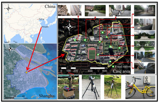
Figure 1.
Location of the case study campus in Shanghai and the distribution map of test sites in the campus.
In this study, nine representative local public spaces of the case study university campus were selected as research areas (as shown in Figure 1) through an integrated consideration of the dimensions of architectural patterns, vegetation types, and spatial morphology. Among them, test site No. 1 is surrounded by low- and medium-rise buildings and lawns. Test site No. 2 is located in the area of medium- and high-rise buildings and test site No. 3 is surrounded by shrubs, grass, and other vegetation. Test site No. 4 is located in the area of mixed buildings of different heights. Test site No. 5 is located in the square in front of tall buildings. Test site No. 6 is surrounded by some buildings and open green areas. Test site No. 7 is surrounded by dense high-rise buildings. Test site No. 8 is surrounded by low- and medium-rise buildings. Test site No. 9 is surrounded by medium- and high-rise buildings. It can be seen that all these nine test sites are lying in different spatial morphology spaces.
3. Methods
3.1. Adoption of Thermal Comfort Index
There are already many thermal comfort indices in the field of outdoor thermal comfort based on the human body heat balance equation, such as Predicted Mean Vote (PMV), NEW standard effective temperature (SET*), Universal Thermal Climate Index (UTCI), and physiological equivalent temperature (PET). Among them, the PET index takes into account environmental factors such as Ta, RH, V, and Tmrt, which can represent people’s thermal perception in the external complex thermal environment more accurately and has a generalized significance [29,30]. A series of studies on the outdoor thermal environment and thermal sensation have adopted the PET index as an evaluation index [31,32,33], and PET has proven to be a useful metric for outdoor comfort in almost all climatic conditions [34]. Therefore, in this study, the physiological equivalent temperature index PET was selected as the human thermal comfort evaluation index and calculated by using RayMan software [35].
3.2. Fixed Weather Station Monitoring
In order to reflect the severe hot summertime climatic conditions with higher temperature and humidity, meteorological days reflecting clear, breezy, and almost cloudless climate characteristics were given priority during the measurement period. By excluding rainy days, the daytime period from 9:00 to 17:00 on 13 August 2017 was selected to conduct the field survey. During the whole survey, the Ta ranged from 27.4 °C to 36.1 °C and the average RH was approximately 75%. The mean V was 1.1 m/s, primarily from the northeast, and the cloud amount derived from on-site manual interpretation was approximately 30%, displaying sunny weather. The background meteorological conditions satisfied the typical climatic characteristics of summertime in Shanghai.
These nine fixed weather stations, numbered 1 to 9, were set at representative surrounding environments that varied substantially between different locations [36,37]. These locations were considered multiple “same” regions by considering the general homogeneity in the geometry layouts and the land cover patterns. A series of necessary meteorological parameters of Ta, RH, V, and globe temperature (Tg) were continuously measured by using real-time recorded weather stations at the nine fixed test sites. The specific parameters of the test instruments are shown in Table 2. The accuracy of these instruments meets the international standard ISO 7726-1998. Based on some relative research and given information from the instrument manufacturers, the use of the globe in the color black was actually reasonable to obtain Tmrt in this study [38,39]. During the test, these instruments were set and recorded every 10s and the sensor probes were placed at 1.5 m pedestrian height.
Table 2.
Instruments of the field survey and their specific parameters.
3.3. Subjective Questionnaire Survey
The subjective questionnaire survey was also conducted simultaneously with fixed weather monitoring. Subjects were randomly selected university students who were around the fixed weather stations. The questionnaire was completed within 2 min to avoid the change in human thermal sensation caused by the thermal environment variations. The questionnaire mainly included subjects’ personal information and thermal sensations. The personal information section covered the subjects’ basic physical conditions (gender, age, weight, height), their state of activity, and clothing thermal resistance. The thermal environment was evaluated by the thermal sensation vote (TSV). The thermal sensation vote adopted a continuous ASHRAE seven-level standard [40] to record the response of the subjects to the thermal environment more clearly. The scale ranged from “-3” to “+3” corresponding to “cold” and “hot”, respectively. A total of 441 sets of questionnaires were obtained, and the proportion of male and female subjects was basically balanced.
Then combining the recorded meteorological data of each test site and the corresponding questionnaire information, the RayMan model was used to calculate the PET values. It should be noted that the calculating process also required the mean radiation temperature (Tmrt), which can be calculated by the following Equation (1) with the measured Ta, Tg, and V. Additionally, this equation focuses on the effect of forced convection on the test site [41].
where Tmrt is the mean radiant temperature, °C. Tg is the globe temperature, °C; V is the wind velocity, m/s. Ta is the air temperature, °C. D is globe diameter (=0.15 m in this study) and ε is emissivity (=0.95 for a black globe).
3.4. Calculation of PET Distributions across the Whole Campus
3.4.1. Spatial Morphology Characteristics
According to Stewart and Oke [36], a local climate zone (LCZ) scheme was developed to quantify the local-scale spatial morphology characteristics. Based on the LCZ parameter system, six spatial morphology characteristic parameters are included: sky view factor (SVF), aspect ratio (AR), height of roughness elements (HRE), building surface fraction (BSF), pervious surface fraction (PSF), and impervious surface fraction (ISF). Among them, the SVF, AR, and HRE reflect the geometry layouts, whereas the BSF, ISF, and PSF describe the land cover patterns. Therefore, these six parameters can generally represent the spatial morphology characteristics of a built-up university campus. The detailed collection and calculation methods for each parameter are shown in Table 3.
Table 3.
Collection and calculation method of surface morphology characteristic parameters.
According to the LCZ classification method, a local zone with a homogeneous land cover layout can be divided into a specific zone. By referring to the underlying surface characteristics of the entire campus, 14 local zones can be divided with consideration of their specific homogeneous spatial morphology, as shown in Figure 2. Based on the calculation methods in Table 3, the surface morphological parameters of each local zone are calculated. Figure 2 also shows the statistical distributions of these six morphological parameters of each local zone.
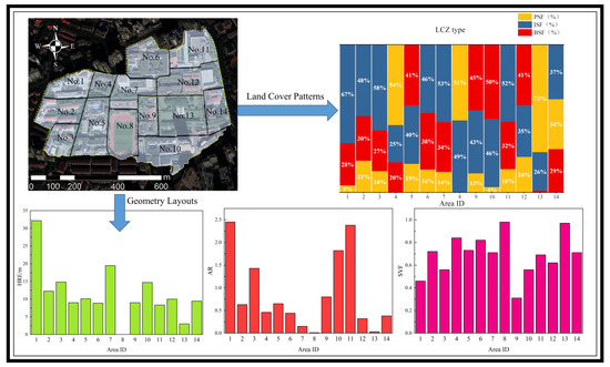
Figure 2.
Local zone divisions within the campus in Shanghai and the distribution chart of spatial morphology characteristic parameters in each local zone.
It can be seen that both the land cover patterns and geometry layouts of these 14 zones varied significantly. First, zones No. 1, No. 2, No. 3, No. 6, No. 7, No. 11, and No. 14 have larger ratios of ISF whereas zones No. 4, No. 8, and No. 13 have larger occupations of PSF. Zones No. 5, No. 9, No. 10, and No. 12 have the most building areas. Second, the SVF shows a wide range from 0.31 to 0.97. Zone No. 9 has the lowest SVF whereas zones No. 8 and No. 13 reach a maximum value of 0.97. The AR generally shows distribution opposite to those of the SVF. Overall, the AR ranges from 0.03 to 2.45, and zone No. 9 has the highest AR, whereas zones No. 8 and No.13 have the lowest AR. In addition, the distribution of the HRE shows values ranging from 0 to 32.17m, of which zone No. 1 has the highest value.
3.4.2. Mobile Measurement
Because the fixed measurement could not continuously cover the whole area across the entire university, the air temperature and humidity data of the whole campus could not be obtained for subsequent correlation analysis. Therefore, in addition to the measurement of meteorological parameters at nine fixed test points, this study further adopted the mobile survey to measure the air temperature (Ta) and relative humidity (RH) across the campus. The mobile survey used a bicycle as the transportation vehicle, trying to maintain a uniform speed (about 15 km/h). The bicycle was equipped with GPS equipment for real-time location recording and a temperature and humidity data logger (HOBO U23-002) for measuring the corresponding thermal environment parameters. The mobile tests were conducted mainly in the daytime from 9:00 to 17:00, and each mobile test was conducted at the beginning of each hour with a test period lasting about 20 min. Eventually, a total of 9 groups of mobile test data were obtained. Figure 3 shows the route of mobile measurement.
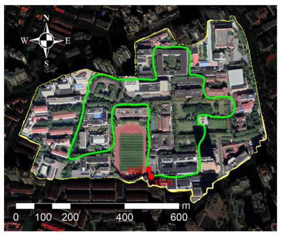
Figure 3.
Mobile measurement roadmap.
After the mobile test, the field air temperature and humidity data obtained by the recorder were matched with the real-time GPS of the mobile route, and the Ta and RH distributions along the mobile measurement route were obtained. Since the position of the Ta and RH data measured in the same mobile route were different, the data were non-simultaneous and time correction was needed before subsequent analysis. This paper adopted a “multiple-distance underlying surface model” (MDUS) [43] to conduct temporal corrections on Ta and RH obtained from the actual mobile test, and the nonuniformity data were corrected to the simultaneous data at a certain moment.
The corrected Ta and RH data were then input into ArcGIS software and their geographic location information was obtained from GPS recorders. Furthermore, with the spatial analysis module in ArcGIS, the spatial interpolation of Ta and RH point data was performed. The distributions of Ta and RH at pedestrian height throughout the university campus were obtained at nine different times.
3.4.3. The PET Calculation Methods across the Whole Campus
Based on the PET calculation method mentioned above, to obtain the PET at nine test sites, the subjects’ personal information and thermal sensation feelings gained by the questionnaire and the Ta, RH, wind speed, and Tmrt measured by the fixed weather station were input into the RayMan software to calculate the hourly PET of each fixed weather station. Then, linear regression analysis was conducted on the relationship between PET, Ta, and RH for subsequent study.
To calculate the PET of 14 zones, firstly, the hourly corrected Ta and RH data of each zone processed in Section 3.4.2 were obtained. Then, based on the linear regression relationship between Ta and RH at the fixed weather stations, the hourly Ta and RH of each zone were used to convert the average PET value of the corresponding zone. Based on the above methods, the PET calculation process framework of the whole campus is shown in Figure 4.
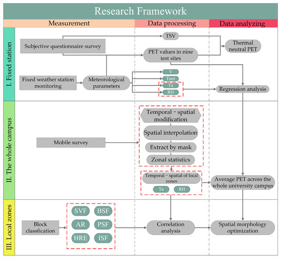
Figure 4.
PET calculation process framework of the whole campus.
4. Results
4.1. Thermal Neutral PET Range of University Students
A total of 441 valid questionnaires were collected, including 252 male samples and 189 female samples. As the survey mainly focused on the university campus, the age of the subjects ranged from 18 to 24 years old. During the test period, the range of clothing thermal resistance was between 0.4 clo and 0.7 clo with an average of 0.48 clo. The human metabolic rate of subjects varied from 58 W/m2 to 200 W/m2, the average value of which was 131.9 W/m2, displaying a medium-intensity exercise level. Table 4 shows the amount and the mean basic attributes of subjects in different test sites.
Table 4.
The basic attributes of the subjects in nine different test sites.
According to the results of outdoor thermal sensation voting (TSV) of the subjects, Figure 5a shows the whole proportion distribution of different subjective thermal sensation evaluations. It can be seen that the subjects feeling “slightly warm” and “warm” were both more than 30%, occupying the majority. A limited proportion of about 15% of the subjects respectively felt “hot” and “neutral” about their surroundings. During the summertime research period, no one felt slightly cold or below. These results indicate that university students have different thermal sensations about the campus thermal environment.
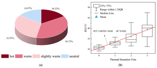
Figure 5.
(a) Proportion distribution of TSV. (b) Statistical results of PET under different TSV scales.
The thermal neutral PET range of these university students during summertime is the main target that would directly guide a thermally comfortable university campus design. Therefore, the correlation regression analysis between PET and the corresponding TSV scales is conducted, as shown in Figure 5b. The distributions show that the PET values have concentrated ranges of TSV scales “2” and “3”. Clear linear correlation relationships between the PET average values and the corresponding TSV scales are revealed with a higher R square of 0.928. It thus illustrates that the PET index could better reflect the subjects’ thermal sensation evaluation.
Here it can be considered that the PET range corresponding to TSV scales varying from “−0.5” to “+0.5” is the thermal neutral PET range [44]. According to the correlation equation, the thermal neutral PET range lies between 29.16 °C and 32.04 °C. The neutral PET ranges of other relevant studies are compared in Figure 6 [8,27,28,45,46,47]. For the summer thermal sensation of university students, the neutral PET ranges in Xi’an and Mianyang of China are significantly different than in the “Cfa” areas. The reason may be that the summer temperature in these two places is lower than that in Cfa. The neutral PET ranges both in Malaysia and this study are higher, which indicates that the students in these two places can better adapt to the warm and humid climate. In the study of other cities in China, although the climate zone in Taiwan is the same as in Wuhan, the Ta and the neutral PET range in Taiwan is higher than that of Wuhan. The mean Ta in Shenzhen is the highest, showing the highest neutral PET range.
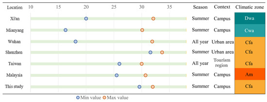
Figure 6.
A comparison of neutral PET ranges in different areas. (Dwa: monsoon-influenced hot-summer humid continental climate; Cwa: monsoon-influenced humid subtropical climate; Cfa: humid subtropical climates; Am: tropical monsoon climate).
4.2. Comparison Analysis of PET Values at Nine Test Sites
The nine fixed test sites have diversified spatial morphology characteristics which resulted in different thermal environment conditions and thus influenced the local human thermal comfort. The mean, minimum, and maximum of thermal environmental data at nine test sites are shown in Table 5. Therefore, the temporal and spatial variations of PET at nine test sites are compared, as shown in Figure 7.
Table 5.
The mean, minimum, and maximum of thermal environmental data at nine test sites.
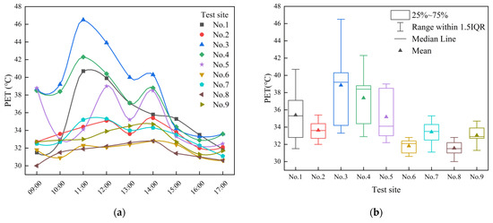
Figure 7.
(a) Hourly variations of PET at nine test sites. (b) PET distributions at nine test sites.
First, the hourly PET variations in Figure 7a show that the PET values in test sites No. 1, No. 3, and No. 4 present obvious upward trends from 11:00 to 14:00. Among them, test site No. 3 presents a relatively long-term high PET condition. The PET curves at test sites No. 6 and No. 8 were relatively flat and always lay at relatively lower PET values during the whole research day. Then, according to the PET spatial statistical distributions in Figure 7b, the PET values at test sites No. 2, No. 6, No. 7, No. 8, and No. 9 all display limited variation ranges from 29.9 °C to 42.5 °C whereas test sites No. 1, No. 3, No. 4, and No. 5 present larger PET variation ranges from 31.8 °C to 46.8 °C. This phenomenon emphasizes that the PET variations are greatly affected by the surrounding environments characterized by their different spatial morphology.
A detailed inspection of the test sites’ surroundings reveals that test sites No. 1 and No. 3 are surrounded by low-rise buildings and shrubs, and test sites No. 4 and No. 5 are located in relatively open spaces with a lower building enclosure degree. Therefore, these test sites are easily influenced by the solar radiation variation due to lacking sufficient shelters. Then, test site No. 6 is surrounded by tall-rise trees which received more appropriate shelter, blocking the solar radiation. Test site No. 8 is surrounded by densely-built buildings with higher enclosures, which also received less solar radiation.
Taken as a whole, the nine test sites with different spatial morphology characteristics greatly influenced the local thermal environment and the outdoor thermal comfort levels of university students. Therefore, a thorough spatial morphology optimization is necessary for improving the campus thermal environment.
4.3. Mobile Survey-Based Temporal–Spatial Thermal Environment Analysis of Local Zones
Based on the Ta and RH measurement results of the synchronously modified nine mobile routes, the spatial averaged Ta and RH of each zone were obtained through spatial interpolation and statistical calculation in ArcGIS. The spatial distributions of Ta and RH at the typical times of 9:00, 14:00, and 17:00 were selected for analysis. The distribution maps at other times were added in Appendix A and Appendix B.
As shown in Figure 8, at 9:00 the Ta values in local zones were generally low and RH values were generally high compared to other times. In addition, the Ta and RH both present relatively smaller spatial differences of 32.34 °C–32.51 °C in Ta and 56.48%–59.63% in RH. Then, at 14:00 the Ta values in local zones were higher and the distribution range was large from 33.86 °C to 37.89 °C. The RH values at 14:00 were also in a larger variation from 51.2% to 56.6%. At 17:00, the Ta and RH values in each local zone were intermediate, which also showed a certain spatial difference.
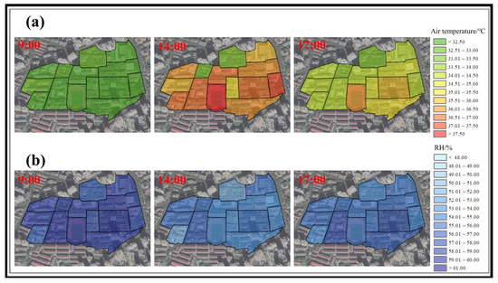
Figure 8.
(a) The temporal and spatial distribution maps of air temperature and relative humidity at typical times in the test area. (a) The distribution maps of air temperature. (b) The distribution maps of relative humidity.
The above phenomenon illustrates that spatial heterogeneity in local zones varied with time, showing the most significance at 14:00 and the least significance at 9:00. Considering the corresponding surrounding environments, the local zones with more open space could receive a large amount of solar radiation but also result in more wind blowing. The effects of green space on a local thermal environment can differ. The tall-rise trees usually provide better shading and help cool the air temperature whereas the low-rise grass and shrubs cannot provide much shelter for local space but have some vegetative transpiration.
4.4. Impacts of Spatial Morphology Characteristic Parameters on Local Thermal Environment
In order to better express the quantitative impacts of spatial morphology characteristics on the local thermal environment of a university campus, the correlation analysis between the spatial morphology characteristic parameters and local Ta and RH at three representative moments of 9:00, 14:00, and 17:00 is conducted, as shown in Figure 9 and Figure 10.
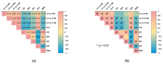
Figure 9.
Correlations between air temperature at specific times and spatial morphology characteristic parameters among the whole campus. (a) Heat map of correlation coefficient. (b) Heat map of significance.
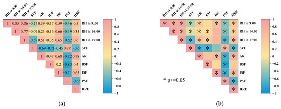
Figure 10.
Correlations between relative humidity at specific times and spatial morphology characteristic parameters among the whole campus. (a) Heat map of correlation coefficient. (b) Heat map of significance.
As shown in Figure 9, the SVF and PSF generally had a positive correlation with Ta, and AR, BSF, PSF, and HRE were negatively correlated with Ta. At 9:00, there was no significant difference between air temperature and these spatial morphology characteristic parameters. The reason may be that the local zone Ta was greatly affected by the background meteorological factors at 9:00. At 14:00 and 17:00, the SVF showed the most positive correlation with Ta, indicating that the zone with high sky openness would receive more radiation heat due to the lack of solar radiation occlusion. The BSF conversely had a strong contribution to the increase in Ta. The reason may be that the vegetation type in these zones were mostly shrubs and low trees, and the shading effects on solar radiation were very weak.
Figure 10 shows that relative humidity was also significantly affected by spatial morphological parameters. Overall, the SVF and PSF generally had a negative correlation with RH, and the AR, BSF, PSF, and HRE were positively correlated with RH. Different from Ta, RH was significantly correlated with the SVF, AR, ISF, PSF, and HRE at 9:00, and was significantly correlated with the SVF, AR, BSF, PSF, and HRE at 14:00 and 17:00, respectively. Based on the calculation formula of Ta and RH, the changing trend of Ta and RH is generally opposite. Therefore, the increase in the building density and height will reduce the Ta and lead to an increase in RH. Taken as a whole, these correlation results emphasized the significant effects of spatial morphology characteristic parameters on the local thermal environment. A reasonable modification for the spatial morphology could effectively relieve the urban thermal environment.
4.5. Spatial Morphology Evaluation of University Campus Based on Thermal Neutral PET Range
As discussed in Section 4.3, the Ta and RH distributions in the study area were obtained. To further quantitatively describe the spatial distribution of outdoor thermal comfort, a multiple linear regression model expressing the relationship of PET, Ta, and RH was conducted, as shown in Equation (2).
It should be noted that this equation was obtained based on the test data during the measurement period with breeze conditions. However, the calculation method had popular significance and was applicable within a certain limit. The correlation analysis revealed that Ta and RH had a significant impact on human outdoor thermal comfort and the PET index can be calculated with these two parameters.
In this way, the PET values of 14 local blocks during the test period were calculated through Equation (2) with Ta and RH, and the total averaged PET integrating nine specific time points were illustrated in Figure 11a. The thermal neutral PET range ranging from 29.16 °C to 32.04 °C was applied to these 14 zones. According to Figure 11b, 12 problem zones whose PET values exceeded the thermal neutral range upper limit of 32.04 °C were identified. Among them, zone No. 8 has the highest PET value of 35.09 °C, which is far more than the thermal neutral limit.
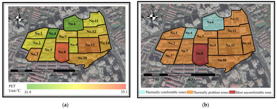
Figure 11.
(a) Spatial distribution map of average PET across the whole university campus. (b) Thermal problem map across the whole university campus.
To quantify the relationships between spatial morphology parameters and human outdoor thermal comfort, the correlations between the spatial morphology parameters and PET were analyzed. The relationships between the SVF, AR, HRE, BSF, ISF, PSF, and PET are shown in Figure 12. The PET increases with increasing SVF and PSF and the decline of AR, HRE, ISF, and BSF. These results show that the blocks with much larger areas of open space and lower buildings or large ranges of natural landscapes with shorter vegetation usually exhibit high PET. Thus, for these problem zones, several suggestions in spatial morphology optimization for improving the students’ outdoor thermal comfort on university campuses during the summertime can be proposed.
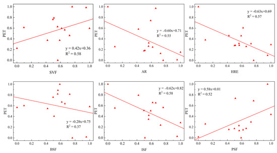
Figure 12.
Linear fitting results of normalized spatial morphology parameters and PET.
From the geometry layout view, the building density, height, and street aspect ratio can be appropriately increased. Higher degrees of enclosure with limited open space are also needed. According to Section 4.4, the high-rise building density and deep street canyons with little open space can achieve effective shading effects which greatly block solar radiation and result in a Tmrt decline. Furthermore, Ta will also decrease and is consequently conducive to the students’ outdoor thermal comfort.
From the land cover pattern view, the low-rise vegetation areas with shrubs and grass usually have weak shading effects on solar radiation with limited transpiration effects. Therefore, tall-rise trees are suggested for distribution throughout the campus space.
5. Conclusions
In this paper, a university campus in Shanghai was selected as the research area. Nine local public outdoor spaces were selected for fixed field climatic measurement on a typical summer day. A subjective questionnaire survey of 441 college students was conducted to calculate the PET thermal comfort index of the campus students. The whole university area was divided into 14 local zones, and the thermal–humid environment was measured through a mobile survey. Several main conclusions of this study were obtained as follows.
Based on the questionnaire information and the measured fixed meteorological data, the PET distributions corresponding to different TSV were obtained. A significant linear relationship between TSV and PET was revealed. A thermal neutral PET range of the college students at outdoor spaces under hot and humid climatic conditions was determined as 29.16 °C to 32.04 °C, which generally accorded with the ranges in other areas of China.
The temporal and spatial variations of PET at nine test sites varied a lot due to their diversified spatial morphology characteristics. The mobile survey measurement results at typical times illustrated the spatial–temporal heterogeneity of Ta and RH in local zones. The Ta and RH both present relatively smaller spatial differences at 9:00 and at 14:00, the distribution range was large in Ta from 33.86 °C to 37.89 °C and from 51.2% to 56.6% in RH.
Correlation analysis between the spatial morphology characteristic parameters and the local Ta and RH shows that the SVF and PSF generally had a positive correlation with Ta, and the AR, BSF, PSF, and HRE were negatively correlated with Ta. Then, the effects of the above spatial morphology characteristic parameters on RH were inverse to that on Ta. With the linear regression model expressing the relationship between PET, Ta, and RH, the averaged PET distributions in the multiple local zones were obtained. Problem zones with higher PET values exceeding the thermal neutral limit were recognized. Suggestions from both the geometry layout view and the land cover pattern view were proposed to guide spatial morphology optimization from the college students’ thermal comfort aspect.
Overall, this study indicates that the local thermal comfort of university students was affected by the spatial morphology characteristics of the university. The planning and design of campuses should consider the geometry layouts and land cover patterns. The results of this study can provide both theoretical reference and technical support for environmentally comfortable university campus design and campus planning. It should be noted that this research was conducted at a specific campus under typical summertime weather conditions. In the near future, more research covering multiple seasons and including more subjects would be conducted to supplement the research applicability.
Author Contributions
L.L. and H.Z. are the main contributors. Conceptualization, L.L. and H.Z.; methodology, L.L. and J.D.; software, Z.L.; validation, J.D.; formal analysis, Z.L.; data, J.D. writing—original draft preparation, L.L. and Z.L.; writing—review and editing, J.L. and H.Z.; visualization, L.L. and Z.L.; funding acquisition, L.L. All authors have read and agreed to the published version of the manuscript.
Funding
This work was supported by Guangzhou Science and Technology Project (Grant No. 202201010274) and Natural Science Foundation of Guangdong Province (Grant No. 2020A1515011092).
Institutional Review Board Statement
Not applicable.
Informed Consent Statement
Informed consent was obtained from all subjects involved in the study.
Data Availability Statement
Not applicable.
Acknowledgments
The authors really appreciate all the participants who have been involved in this field survey under the hot and humid climatic conditions.
Conflicts of Interest
The authors declare no conflict of interest.
Appendix A

Figure A1.
Hourly air temperature maps in the university campus region.
Figure A1.
Hourly air temperature maps in the university campus region.

Appendix B

Figure A2.
Hourly relative humidity maps in the university campus region.
Figure A2.
Hourly relative humidity maps in the university campus region.

References
- Nutsford, D.; Pearson, A.L.; Kingham, S. An Ecological Study Investigating the Association between Access to Urban Green Space and Mental Health. Public Health 2013, 127, 1005–1011. [Google Scholar] [CrossRef] [PubMed]
- Wolch, J.R.; Byrne, J.; Newell, J.P. Urban Green Space, Public Health, and Environmental Justice: The Challenge of Making Cities “Just Green Enough”. Landsc. Urban Plan. 2014, 125, 234–244. [Google Scholar] [CrossRef]
- Hajrasouliha, A.; Ewing, R. Campus Does Matter: The Relationship of Student Retention and Degree Attainment to Campus Design. Plan. High. Educ. 2016, 44, 30–45. [Google Scholar]
- Shamsuddin, S.; Bahauddin, H.; Aziz, N.A. Relationship between the Outdoor Physical Environment and Student’s Social Behaviour in Urban Secondary School. Procedia-Soc. Behav. Sci. 2012, 50, 148–160. [Google Scholar] [CrossRef]
- Hanan, H. Open Space as Meaningful Place for Students in ITB Campus. Procedia-Soc. Behav. Sci. 2013, 85, 308–317. [Google Scholar] [CrossRef]
- Rashid, M.; Obeidat, B. Students’ Static Activities in Relation to Campus Quad Design and Layout. Exploring Gender-Based Differences. J. Public Space 2020, 5, 75–94. [Google Scholar] [CrossRef]
- Alnusairat, S.; Ayyad, Y.; Al-Shatnawi, Z. Towards Meaningful University Space: Perceptions of the Quality of Open Spaces for Students. Buildings 2021, 11, 556. [Google Scholar] [CrossRef]
- Huang, Z.; Cheng, B.; Gou, Z.; Zhang, F. Outdoor Thermal Comfort and Adaptive Behaviors in a University Campus in China’s Hot Summer-Cold Winter Climate Region. Build. Environ. 2019, 165, 106414. [Google Scholar] [CrossRef]
- Lai, A.; Maing, M.; Ng, E. Observational Studies of Mean Radiant Temperature across Different Outdoor Spaces under Shaded Conditions in Densely Built Environment. Build. Environ. 2017, 114, 397–409. [Google Scholar] [CrossRef]
- Jamei, E.; Rajagopalan, P.; Seyedmahmoudian, M.; Jamei, Y. Review on the Impact of Urban Geometry and Pedestrian Level Greening on Outdoor Thermal Comfort. Renew. Sustain. Energy Rev. 2016, 54, 1002–1017. [Google Scholar]
- Achour-Younsi, S.; Kharrat, F. Outdoor Thermal Comfort: Impact of the Geometry of an Urban Street Canyon in a Mediterranean Subtropical Climate—Case Study Tunis, Tunisia. Procedia-Soc. Behav. Sci. 2016, 216, 689–700. [Google Scholar] [CrossRef]
- Liu, Y.; Li, H.; Gao, P.; Zhong, C. Monitoring the Spatiotemporal Dynamics of Urban Green Space and Its Impacts on Thermal Environment in Shenzhen City from 1978 to 2018 with Remote Sensing Data. Photogramm. Eng. Remote Sens. 2021, 87, 81–89. [Google Scholar] [CrossRef]
- Fei, F.; Wang, Y.; Yao, W.; Gao, W.; Wang, L. Coupling Mechanism of Water and Greenery on Summer Thermal Environment of Waterfront Space in China’s Cold Regions. Build. Environ. 2022, 214, 108912. [Google Scholar] [CrossRef]
- Chen, J.; Wang, H.; Zhu, H. Analytical Approach for Evaluating Temperature Field of Thermal Modified Asphalt Pavement and Urban Heat Island Effect. Appl. Therm. Eng. 2017, 113, 739–748. [Google Scholar] [CrossRef]
- Liu, X.; Cao, J.; Xin, D. Wind Field Numerical Simulation in Forested Regions of Complex Terrain: A Mesoscale Study Using WRF. J. Wind Eng. Ind. Aerodyn. 2022, 222, 104915. [Google Scholar] [CrossRef]
- Molnár, G.; Kovács, A.; Gál, T. How Does Anthropogenic Heating Affect the Thermal Environment in a Medium-Sized Central European City? A Case Study in Szeged, Hungary. Urban Clim. 2020, 34, 100673. [Google Scholar] [CrossRef]
- He, C.; Zhou, L.; Yao, Y.; Ma, W.; Kinney, P.L. Estimating Spatial Effects of Anthropogenic Heat Emissions upon the Urban Thermal Environment in an Urban Agglomeration Area in East China. Sustain. Cities Soc. 2020, 57, 102046. [Google Scholar] [CrossRef]
- Yaglou, C.P.; Minard, D. Control of Heat Casualties at Military Training Centers. AMA Arch. Ind. Health 1957, 16, 316–320. [Google Scholar]
- Ole Fanger, P. Thermal Comfort. Analysis and Applications in Environmental Engineering; Copenhagen Danish Tech. Press: Copenhagen, Denmark, 1970. [Google Scholar]
- Gagge, A.P.; Fobelets, A.P.; Berglund, L.G. Standard Predictive Index of Human Response to the Thermal Environment. ASHRAE Trans. 1986, 92, 709–731. [Google Scholar]
- Höppe, P. The Physiological Equivalent Temperature—A Universal Index for the Biometeorological Assessment of the Thermal Environment. Int. J. Biometeorol. 1999, 43, 71–75. [Google Scholar] [CrossRef]
- Jendritzky, G.; Maarouf, A.; Fiala, D.; Staiger, H. An Update on the Development of a Universal Thermal Climate Index. In Proceedings of the 15th Conference on Biometeorology and Aerobiology Joint with the 16th International Congress on Biometeorology, Kansas City, MO, USA, 28 October–1 November 2002. [Google Scholar]
- Fang, Z.; Feng, X.; Liu, J.; Lin, Z.; Mak, C.M.; Niu, J.; Tse, K.T.; Xu, X. Investigation into the Differences among Several Outdoor Thermal Comfort Indices against Field Survey in Subtropics. Sustain. Cities Soc. 2019, 44, 676–690. [Google Scholar] [CrossRef]
- Wu, J.; Liu, C.; Wang, H. Analysis of Spatio-Temporal Patterns and Related Factors of Thermal Comfort in Subtropical Coastal Cities Based on Local Climate Zones. Build. Environ. 2022, 207, 108568. [Google Scholar] [CrossRef]
- Zhang, Z.; Dong, J.; He, Q.; Ye, B. The Temporal Variation of the Microclimate and Human Thermal Comfort in Urban Wetland Parks: A Case Study of Xixi National Wetland Park, China. Forests 2021, 12, 1322. [Google Scholar] [CrossRef]
- Chen, X.; Gao, L.; Xue, P.; Du, J.; Liu, J. Investigation of Outdoor Thermal Sensation and Comfort Evaluation Methods in Severe Cold Area. Sci. Total Environ. 2020, 749, 141520. [Google Scholar] [CrossRef]
- Othman, N.E.; Zaki, S.A.; Rijal, H.B.; Ahmad, N.H.; Razak, A.A. Field Study of Pedestrians’ Comfort Temperatures under Outdoor and Semi-Outdoor Conditions in Malaysian University Campuses. Int. J. Biometeorol. 2021, 65, 453–477. [Google Scholar] [CrossRef]
- Niu, J.; Hong, B.; Geng, Y.; Mi, J.; He, J. Summertime Physiological and Thermal Responses among Activity Levels in Campus Outdoor Spaces in a Humid Subtropical City. Sci. Total Environ. 2020, 728, 138757. [Google Scholar] [CrossRef]
- Jin, H.; Qiao, L.; Cui, P. Study on the Effect of Streets’ Space Forms on Campus Microclimate in the Severe Cold Region of China—Case Study of a University Campus in Daqing City. Int. J. Environ. Res. Public Health 2020, 17, 8389. [Google Scholar] [CrossRef]
- Taleghani, M. The Impact of Increasing Urban Surface Albedo on Outdoor Summer Thermal Comfort within a University Campus. Urban Clim. 2018, 24, 175–184. [Google Scholar] [CrossRef]
- Ma, X.; Zhang, L.; Zhao, J.; Wang, M.; Cheng, Z. The Outdoor Pedestrian Thermal Comfort and Behavior in a Traditional Residential Settlement—A Case Study of the Cave Dwellings in Cold Winter of China. Sol. Energy 2021, 220, 130–143. [Google Scholar] [CrossRef]
- Lai, D.; Guo, D.; Hou, Y.; Lin, C.; Chen, Q. Studies of Outdoor Thermal Comfort in Northern China. Build. Environ. 2014, 77, 110–118. [Google Scholar] [CrossRef]
- Yang, W.; Wong, N.H.; Zhang, G. A Comparative Analysis of Human Thermal Conditions in Outdoor Urban Spaces in the Summer Season in Singapore and Changsha, China. Int. J. Biometeorol. 2013, 57, 895–907. [Google Scholar] [CrossRef] [PubMed]
- Abdollahzadeh, N.; Biloria, N. Outdoor Thermal Comfort: Analyzing the Impact of Urban Configurations on the Thermal Performance of Street Canyons in the Humid Subtropical Climate of Sydney. Front. Arch. Res. 2020, 10, 394–409. [Google Scholar] [CrossRef]
- Matzarakis, A.; Rutz, F.; Mayer, H. Modelling Radiation Fluxes in Simple and Complex Environments: Basics of the RayMan Model. Int. J. Biometeorol. 2010, 54, 131–139. [Google Scholar] [CrossRef]
- Stewart, I.D.; Oke, T.R. Local Climate Zones for Urban Temperature Studies. Bull. Am. Meteorol. Soc. 2012, 93, 1879–1900. [Google Scholar] [CrossRef]
- Liu, L.; Lin, Y.; Liu, J.; Wang, L.; Wang, D.; Shui, T.; Chen, X.; Wu, Q. Analysis of Local-Scale Urban Heat Island Characteristics Using an Integrated Method of Mobile Measurement and GIS-Based Spatial Interpolation. Build. Environ. 2017, 117, 191–207. [Google Scholar] [CrossRef]
- Oliveira, A.V.M.; Raimundo, A.M.; Gaspar, A.R.; Quintela, D.A. Globe Temperature and Its Measurement: Requirements and Limitations. Ann. Work. Expo. Health 2019, 63, 743–758. [Google Scholar] [CrossRef]
- Lam, C.K.C.; Cui, S.; Liu, J.; Kong, X.; Ou, C.; Hang, J. Influence of Acclimatization and Short-Term Thermal History on Outdoor Thermal Comfort in Subtropical South China. Energy Build. 2021, 231, 110541. [Google Scholar] [CrossRef]
- ANSI/ASHRAE ANSI/ASHRAE Standard 55-2017; Thermal Environmental Conditions for Human Occupancy. ASHRAE Inc.: Atlanta, GA, USA, 2017.
- Teitelbaum, E.; Alsaad, H.; Aviv, D.; Kim, A.; Voelker, C.; Meggers, F.; Pantelic, J. Addressing a Systematic Error Correcting for Free and Mixed Convection When Measuring Mean Radiant Temperature with Globe Thermometers. Sci. Rep. 2022, 12, 6473. [Google Scholar] [CrossRef]
- Bernard, J.; Bocher, E.; Petit, G.; Palominos, S. Sky View Factor Calculation in Urban Context: Computational Performance and Accuracy Analysis of Two Open and Free GIS Tools. Climate 2018, 6, 60. [Google Scholar] [CrossRef]
- Liu, L.; Lin, Y.; Wang, D.; Liu, J. An Improved Temporal Correction Method for Mobile Measurement of Outdoor Thermal Climates. Arch. Meteorol. Geophys. Bioclimatol. Ser. B 2017, 129, 201–212. [Google Scholar] [CrossRef]
- Liu, W.; Zhang, Y.; Deng, Q. The Effects of Urban Microclimate on Outdoor Thermal Sensation and Neutral Temperature in Hot-Summer and Cold-Winter Climate. Energy Build. 2016, 128, 190–197. [Google Scholar] [CrossRef]
- Ye, X.; Chen, F.; Hou, Z. The Effect of Temperature on Thermal Sensation: A Case Study in Wuhan City, China. Procedia Eng. 2015, 121, 2149–2156. [Google Scholar] [CrossRef]
- Liu, L.; Lin, Y.; Wang, D.; Liu, J. Quantitative Analysis of the Outdoor Thermal Comfort in the Hot and Humid Summertime of Shenzhen, China. J. Harbin Inst. Technol. 2017, 24, 30–38. [Google Scholar] [CrossRef]
- Lin, T.P.; Matzarakis, A. Tourism Climate and Thermal Comfort in Sun Moon Lake, Taiwan. Int. J. Biometeorol. 2008, 52, 281–290. [Google Scholar] [CrossRef]


Publisher’s Note: MDPI stays neutral with regard to jurisdictional claims in published maps and institutional affiliations. |
© 2022 by the authors. Licensee MDPI, Basel, Switzerland. This article is an open access article distributed under the terms and conditions of the Creative Commons Attribution (CC BY) license (https://creativecommons.org/licenses/by/4.0/).