Abstract
Anthropogenic heat (QF) is one of the parameters that contributes to the urban heat island (UHI) phenomenon. Usually, this variable is studied holistically, among other anthropogenic flux such as industrial, vehicular, buildings, and human metabolism, due to the complexity of data collection through field measurements. The aim of this paper was to weigh vehicular anthropogenic heat and its impact on the thermal profile of an urban canyon. A total of 108 simulations were carried out, using the ANSYS Fluent® software, incorporating variables such as the number of vehicles, wind speed, urban canyon orientation, and urban canyon aspect ratio. The results were compared with a database of 61 American cities in 2015 and showed that orientation is the main factor of alteration in vehicular heat flow, increasing it in a range of 2 °C to 6.5 °C, followed by the wind speed (1.2 to 2.2 m/s), which allows for decreases of 1 to 3.8 °C. The exploration of these variables and their weighing in the definition of urban street canyon temperature profiles at the canopy level of urban structures provides valuable information on the hygrothermal comfort of its inhabitants; its appropriate quantification can be an example of many urban energy balances altering processes.
1. Introduction
The urban heat island (UHI) phenomenon refers to the high-temperature peaks within a city, compared to its surrounding areas, affecting the comfort and health of the inhabitants in urbanized areas that currently amount to 54% (3888 million) of the current world population and, according to the United Nations report for the year 2050, with its demographic growth combined with migration, will be 66% (6336 million) [1].
Therefore, the study of the UHI has developed several lines of research: (a) those referring to its measurement and prediction, (b) the analysis of the influence of the variants that cause it, together with its weighting [2,3], and (c) from the perspective of the energy balance, the development of strategies and techniques to mitigate the intensity of the UHI.
Currently, large-scale measurements that focus on obtaining information from UHI isotherms have gained ground with remote sensing; however, these values are focused on the surface UHI that have served as a means of comparison for the UHI located in the canopy. Additionally, microscale studies are considered a reflection of the behavior of a city, using them to determine and measure the effectiveness of adaptation strategies in a small-scale defined area, according to the environmental conditions of a given place [4,5,6,7,8,9], where this information is taken as input for software development or predictive models.
The information collected from macro and micro-scale climate measurements provides insights into the physical phenomena affecting the built environment. It constitutes a wealth of knowledge for urban planners, whether public or private, that is necessary for research focused on current energy efficiency issues, comfort, health, and stress, as well as a thermal adaptation that affects psychological and physical aspects of the inhabitants in urban areas [4,10].
Regarding strategies or mitigation techniques, research ranges from cool materials with the characterization of their thermal properties (reflectance, albedo, thermochromic, and thermal storage capacity), vegetation systems and bodies of water using evapotranspiration, the reduction of energy inputs [11], and proposals for urban design and land use, such as those proposed in the geometry and profiles of cities harnessing natural and forced convection, as well as shade.
Parameters that weigh the thermal values of the UHI are:
- (a)
- The thermal properties of city surfaces;
- (b)
- Urban morphology ranges from land use, location, orientation, sky view factor, and building profiles to their geometric shape;
- (c)
- The synoptic meteorological parameters: dry bulb temperature, relative humidity, radiation, wind speed, and those currently studied, such as precipitation, cloud cover, fog, air pollution, and mist [3,11,12];
- (d)
- The anthropogenic heat (QF) is analyzed holistically with the heat flows of the human metabolism, industry, application of mechanical systems for comfort in interior spaces, and vehicles (QFV).
It should be noted that advective fluxes, as well as latent and sensible heat generated by these anthropogenic sources, are considered the main causes of the interaction between heat waves and UHI [13].
The first approach to the study of QFV flow was used as a synonym for energy consumption [14], where its incorporation in the urban climate simulation models was relatively simple and generally included as a constant in the energy budget equations of surface volume and control volume. One way to estimate the heat released by vehicles on a mesoscale is through statistical methods. Sailor [15] estimated heat emissions based on energy budget closure and energy models. However, according to the author, these must be validated with micrometeorological measurements. The suggestion regarding the QFV was a specific analysis that allows the creation of a modelling technique to determine the spatial profiles of the vehicles’ heat emissions.
The inclusion of QF in the energy-efficient models of buildings is generally provided by an anthropogenic heating profile of systems, such as the weather research and forecasting (WRF) model, where the values for commercial categories, high-density residential, and low-density residential are 90, 50, and 20 W m−2, respectively. In the modeling challenges of the urban heat island and its components, Mirzaei [16] confirms that the impact of different parameters, such as aspect ratio, orientation, surface properties of materials in the envelopes, and even vegetation can be analyzed through the Computational Fluid Dynamics (CFD), which uses the Navier–Stokes equations. However, due to the high computational cost, care must be taken in the domain size delimitation.
Through transient and stationary CFD simulations with experimental validations, the work of Bottillo et al. [17] addressed the issue of solar radiation and thermal parameters within urban canyons, presenting an analysis dynamic of the factors on the heat transfer coefficient and considering the equations of momentum, continuity, and heat conservation. The results of this investigation highlighted that the heat transfer coefficient in leeward walls is less accentuated than in walls exposed to the sun, increasing from 7.1 to 10.5 w/m2 k.
Another example is the study by Gagliano et al. [18], where thermal behavior was analysed using the CFD software of three urban canyons with aspect ratios H/W = 1.0. Aspects such as reflectance, wind speed, and orientation were varied. In the study, two-dimensional equations were considered: a steady-state, Reynolds-averaged Navier–Stokes (RANS) through the FLUENT code and the alternate albedo coefficients, which were 0.7 and 0.2, thus providing essential data that the high albedo coefficient adopted in the materials used in the building envelope guaranteed a decrease of 1.5 °C in the ambient temperature.
For the understanding of the thermal behavior in an urban canyon, another critical factor to consider is that of anthropogenic vehicular heat and its direct effect on diffuse radiation. Grajeda et al. [19,20] carried out different simulations with CFD and field validations. The variables used included vehicle capacity, orientation, and, in the second case, wind speed. In conclusion, the authors mentioned that vehicles increased the ambient temperature by up to 26% when the orientation of the canyons was from North to South, compared to the east–west orientation.
A work of global estimation of anthropogenic heat is the one presented by Jin et al. [21], where they analysed the relationship of QF with the net surface solar radiation and surface heat island through the methodology of the inventory approach, comparing the data between the years 1980 and 2018 of the 100 largest cities in the world. Among its conclusions, it states that there was an increase of 0.07 to 0.15 W m−2 at a global level. In the case of China, for every 1.0 W/m2 it means an increase of 0.0275 °C associated with surface temperature in urban areas.
Takahashi et al. [22] made simultaneous measurements in three areas (a commercial area with low-rise buildings, university green area, and square slab covered with concrete) to determine and validate the heat flux through the (CFD) software. They developed a model combining the exchange of surface radiation and calculation of non-steady-state heat transfer of the walls and floors of buildings. During the procedure, the air temperature, surface temperature of building walls and streets, solar radiation, long-wave radiation, sensible heat flux, and latent heat flux were considered. From the results obtained, between the measured and simulated values, the average difference in surface temperature on walls and floors was 2.1 °C, and the average difference in urban air temperature was +0.3 °C.
In China, a remote sensing and socioeconomic data study were conducted in the Yangtze River Delta region in a south-eastern region. It was stated that the amount of anthropogenic heat reached 2.38 W m−2 in 2015, thus indicating that different human activities contribute to different QF values [23].
Although the QF profiles are user-editable, anthropogenic heat data on any of its components (industry, vehicle, building, and metabolism) are not available for many cities, thus increasing the likelihood that users will use the QF profiles without changes. In some cases, the lack of these data leads urban modelers to disable QF magnitudes (e.g., [24]) or use custom profiles that neglect some key emissions components, such as the vehicle sector [25].
Using energy consumption inventory methods, some researchers have calculated anthropogenic heat estimates in the order of 10–100 W m−2 for cities as diverse as Lodz, Poland, and Philadelphia, USA [26]. Meanwhile, Chow and Sailor [27] sought to estimate these values in a more detailed way for various regions, using them with the variables of time and place, in order to generate an anthropogenic database for sustainable urban planning. The analyses of specialists such as Sailor and Lu [28] suggested that, in cities such as Houston, USA, the total heating of the vehicle sector is 300 W m−2 during the afternoon rush hour on 500 m grids located on the main streets. Finally, Sailor et al. [26] affirmed that the magnitude of QFV is a function of the spatial extension of the area of analysis, thus adding the urban forms and functions that depend on the energy consumption, traffic patterns, and microclimate.
However, there are few studies that analyze the value of QFV disassociated from the other heat fluxes, since it is considered difficult to measure and calculate because it varies with time and space [15]. This endeavor requires a large amount of official data (for example: analysis grid identifiers, total number of streets, type of vehicle, gasoline/diesel distribution, annual average daily traffic flow, daytime traffic flow profile, kilometers traveled by group of vehicles and grid, emissions function by vehicle group and road type, speed on different road classes, and fleet composition by emissions standard), such as those used in research for cities in the UK, Singapore, Phoenix, and Beijing [21,23,27,29,30,31], which are not always complete or available from government agencies in cities with smaller populations.
The importance of this research lies in the fact that the contribution of the QFV heat flux can also be analyzed in a simulated environment, being verified with field measurement, which indicates that the results have an acceptable degree of certainty, without requiring quantified global values for long periods.
It is also verified that the high contribution of QFV as a heat source towards indoor spaces must be considered in energy efficiency analyses, studies of outdoor areas that affect parameters such as the physiological equivalent temperature, and the designs of both the built envelopes and urban facilities that allow heat flows generated by anthropogenic activities to be controlled and dissipated effectively [32].
2. Materials and Methods
2.1. Study Case
At the microscale, the analyzed area is Independencia Avenue, which is the main avenue of the historic downtown of the city of Veracruz, Mexico. Its geographical location is latitude 19°10′51″ North, longitude 96°08′34″ West, and its altitude above sea level is 15 m (Figure 1). Since the 90’s, there has been a decrease in the population of the historic center towards the periphery of the urban sprawl, reaching a figure of almost 60% by the year 2010. This phenomenon has produced neglect of the urban and architectural heritage downtown, thus generating a high rate of abandoned homes but that has brought with it a growth in commercial centers, consolidating the current urban structure of downtown Veracruz, which is increasing 13% each year [33]. In the 19th and 20th centuries, buildings that presented a structural risk were demolished, so their construction system is made with contemporary materials, such as clay, concrete, steel, and glass partitions, maintaining a maximum height of 20 m in most cases [34].
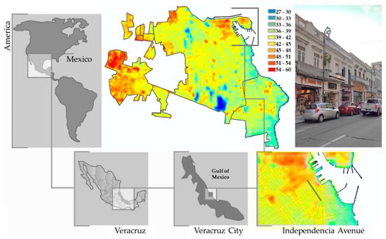
Figure 1.
Location of the case study, map of isotherms (values in °C) of the superficial urban heat island of the metropolitan area of Veracruz and Boca del Rio on 4 May 2017, and photograph of the area.
Veracruz has a tropical climate, with rain in summer, classified as Aw2 (Hot, humid climate greater than 55.3% RH) by Köppen-Geiger [35]. The average annual temperature is 28 °C, with maximums and minimums of 35 and 20 °C, the average, maximum, and minimum RH are 80%, 89%, and 67%, respectively, and a yearly average rainfall of 1516 mm/year, with maximum monthly values of 360 mm in July. Veracruz was selected because it has a predisposition for a temperature increase of 0.59 °C per decade, a deduction calculated from 30 years of measurements provided by the Gulf Basin Agency, Veracruz, Mexico, a certified center and the most important in the metropolitan area [36].
The urban canyon case was selected, due to the following factors:
- (a)
- Analysis of the Urban Heat Island with images of thermal bands 10 and 11 of LandSat 8 for one year using Tomlinson et al. [37], Anderson et al. [38], Mia et al. [39], and Grajeda et al. [40]‘s methodologies.
- (b)
- Analysis of the coating of paved surfaces [41].
- (c)
- Analysis of traffic behavior patterns with statistical information from the Center for Sustainable Transportation in Mexico [42].
- (d)
- Urban canyon aspect ratio analyses in compliance with H/W ≥ 1 = 1 or higher.
- (e)
- Determination of the area as Urban Zone 2, according to World Meteorological Organization guidelines [43].
- (f)
- Orientation of the street, which must be North to South, according to WMO [43], thus indicating the presence of shading/sunshine in streets with this orientation are preferable to those of east-west orientation for the realization of climatic measurements.
- (g)
- Determination of the period for field measurements.
2.2. Data Collected
The equipment used was the SHT75 sensor to measure temperature and relative humidity, with a precision of T = ± 0.3 °C and RH = ± 1.8%, resolution of T = 0.01 °C and RH = 0.05%, response time T = 5–30 s, and RH = 8 s with operating temperature from −40 °C to 123.8 °C, installed on a Phantom 3 drone with operating parameters from −10 to 50 °C, maximum load of 0.5 kg, maximum rate of climb and descent of 6 m/s, the maximum flight speed of 10 m/s, a flight time of 15 minutes for data collection, and with a rotary-wing type propulsion/lift system at the top [36]. In addition, measurements with the drone were specified in three positions, X, Y, and Z, to obtain hexagonal mesh type data to be compared with the simulation.
On the X-axis, the number of measurements was determined by the number of lanes; however, a minimum of three points is considered, with two located on the sides of the facades at 1.5 m and one at the middle of the street. On the Z-axis, the number is defined according to the levels; in this case, two points with a height of 1.5 and 3.0 m are considered. On the Y-axis, the number of data was determined by the length of the urban canyon and flight time of the drone, considering a measurement every 1 m giving a total of 91 data. In the end, the total of measurements between the three axes (X = 3, Z = 2 and Y = 91) per day were 546 data, values that were later taken for the validation of the model (see Figure 2).
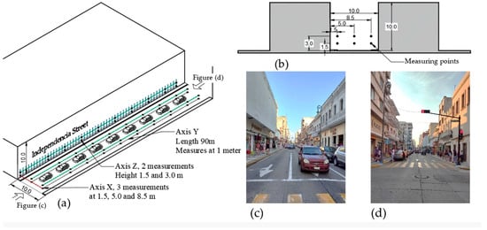
Figure 2.
(a) Isometric of the urban canyon locating the axes X, Y, and Z. (b) Section with dimensions of the “in situ” measurements. (c) View from south to north of the street. (d) North view of the street.
Measurements were taken on 19–20 May 2018 (warm period with 32 °C), and on 2–3 February 2019 (semi-warm period with 29 °C), at 13:30 h, so the western façade already had a 30-minute solar exposure. In both campaigns, measurements were carried out in a two-day period (Saturday and Sunday) to have values characterizing different vehicular traffic patterns, approximately 10 and 6 vehicles per minute, respectively.
2.3. CFD Modeling
The commercial CFD code ANSYS Fluent 15.1 [44] was used in this study to simulate the heat flux of motor vehicles and their contribution to air temperature oscillation in the urban environment, specifically in urban canyons. In addition, a sensitivity analysis was conducted to determine the impact of variations in urban canyon orientation, urban canyon aspect ratio (width/height), wind speed, and the number of vehicles on the temperature profiles of the urban canyon.
2.3.1. Computational Geometry and Grid
A 3D model was made of the urban canyon delimited by two city blocks. The computational domain is defined by dimensions of 190 × 180 × 60 m (length, width, and height); the featured rectangular prisms (city blocks) of 100 (length) × 50 m (width) have varying height values of 10 and 20 m. The width of the canyon, that is, the separation between both prisms, also varies from 10 to 20 m, resulting in two aspect ratios H/W (height of buildings divided by the width of the street) in the simulations. Additional geometry was defined for the motor vehicles (cars), with dimensions of 4.0 × 2.0 × 1.5 m3 (Figure 3a).
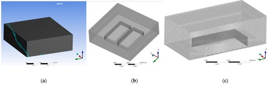
Figure 3.
(a) Computational domain (dimensions in meters); (b) computational grid (720,000 cells); (c) grid section of urban canyon.
From data obtained in the field measurements, the maximum number of cars is 20 units (100%), which is the local standard vehicle capacity per street; subsequent simulations were carried out with 10 and 0 cars to represent the quartiles of 100%, 50%, and 0%, respectively, and determine the thermal behaviour of the urban canyon. Wind speed values of 1.2 and 2.2 m/s were considered the mean and maximum values, respectively, as recorded during the field campaign. A total of 108 simulations were carried out, considering the parameters in Table 1.

Table 1.
Simulation variables and its values.
Geometry and grid generation was executed with the pre-processors design modeler and fluent meshing in the ANSYS workbench, resulting in a grid with 2,060,565 nodes, 1,994,508 elements, and 720,000 cells, respectively. The selected configuration is based on its perfect adaptation to the geometry of the simulation domain, and an example can be found in [45] (Figure 3c). The resolution of the grid went through a sensitivity analysis, in quality from coarse to fine (120,000 to 1,680,000 cells), where results show a difference of less than 0.5%. A total of 500 iterations were run to converge in the solution or have residuals less than 10−3 in the values, according to the criteria provided in the ANSYS theory references [44].
A mesh with fine relevance is selected, and slow transitions are chosen in response to the difference in surface area of the combined geometry in the model to save computational resources, without compromising accuracy in the results.
2.3.2. Boundary Conditions
The boundary conditions determined for this model were (A) inlet with a uniform profile of wind velocity, according to measured data (0, 1.2, or 2.2 m/s), with a turbulence intensity of 5% in the inlet flow- turbulent kinetic energy, and turbulence dissipation rates of 1.0 and 1.2, respectively. The thermal boundary condition at the inlet is a constant temperature equal to the annual average mean temperature of the case study, Independencia Avenue, 30 °C. (B) The walls of the computational domain were defined with the symmetry condition and modeled as no-slip walls with standard roughness. Scalable wall functions were applied. (C) Outlet plane was set with zero static gauge pressure. (D) Solid opaque materials were geometry generated for the surfaces that define the urban canyon, buildings, and pavement. (E) Within the geometry modeled for the vehicles, the car hood was set at a constant temperature of 60 °C, according to Cascetta et al. [46], which measured the internal and external temperatures of a vehicle to determine its average radiant temperature (Figure 3a,b).
The materials used in the simulations are those found in the case study: metal sheet in the auto body, hydraulic concrete for the pavement, and cement plaster for the building envelope. The physical characteristics and thermal properties are listed in Table 2.
Table 2.
Thermal properties of materials used (source: [47]).
2.3.3. Solver Settings
The present model assumes a constant isotropic heat flow with specific viscosity characteristics; therefore, the Reynolds-averaged Navier–Stokes (RANS) equations were used [44]. A steady-state simulation is determined because the input values correspond to a set moment (specific day and time), where the components are stable over time. The control volume was defined as an ideal gas.
In the simulations, two models were activated, i.e., K-ε realizable and surface-to-surface radiation (S2S). For the modeling of the canopy layer, the K-ε realizable model was considered appropriate to ensure adequate representation of wind viscosity in the model walls, as well as the application of a precise equation for the transport of the squared vorticity fluctuation. The model was validated in the works of Yuan et al. [48] and Aghamolaei et al. [49].
The radiation model surface-to-surface (S2S) calculated the direct and diffuse radiation from the solar position vector generated with the data of the case study (longitude 96.13° W y latitude 19.17° N), resulting in 884.78, 72.57, 118.56, and 99.58 W m−2 for direct, vertical diffuse, horizontal diffuse, and reflected radiation, respectively, for the date of 19 May at 13:00 h. Energy flux calculated by ANSYS FLUENT [44] is based on the sum of all reflected energy (Equation (1)) and fraction of the incident energy on one surface from another, the view factor (Equation (2)).
where:
- qout,k = energy flux leaving the surface
- εk = emissivity
- = Stefan–Boltzmann constant
- qin,k = energy flux incident on the surface from the surroundings
- Ak = surface area;
- Fjk = view factor between surface k and surface j;
- q = energy flux incident on the surface.
2.3.4. CFD Results
Temperature values were obtained through line probes, with 100 measurement points spaced equidistantly along the modeled geometry at 1.5 and 3 m in height. There were six (6) line probes in the urban canyon; four were set near the building walls (1.5 m), and two were set at the center of the urban canyon. This array allows for the analysis of the internal temperature profile of the canyon (Figure 4) [19].
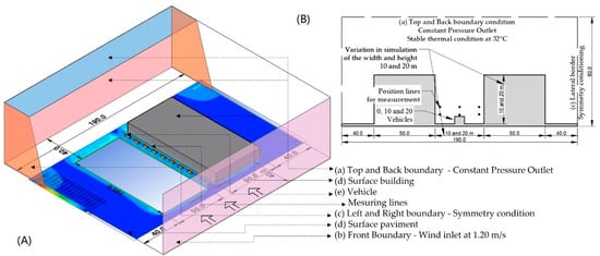
Figure 4.
(A) Isometric indicating boundary conditions. (B) Section with general measurements for data location, as well as the general volume of the domain.
2.4. Simulation Validation
The index used for the validation of the simulation data versus the field measurements is the percent mean absolute relative error (PMARE). Ali and Abustan [50] explained that the PMARE presents less ambiguity and is logical, simple, and interpretable, basing its results on quantitative and statistical methods. This index was specifically designed to validate simulation through field measurements. RMSE quantifies the dispersion between simulation and field measurements, matching it with models such as mean error (ME), mean absolute error (MAE), and root mean square error (RMSE). The range of the other index varies from 0% to ∞ (positive infinity), with 0.0 being the optimal value, and higher values indicate a more significant error; meanwhile, the PMARE could variate between 0 and hundred giving a parameter of how the agreement is. The equation used was:
where:
- PMARE = percent mean absolute relative error;
- Abs = absolute value (of the difference between observed and simulated value);
- n = number of observations;
- Oi = observed value in field;
- Pi = simulated value.
The comparison data were those of the simulation with ten vehicles, width, height of 10m, and wind speed of 1.2 m/s, against the data of the field campaign of 19 May 2018 (10 cars and wind of 1.2 m/s). From the monitored urban canyon, a section of two blocks was chosen due to its geometric properties, street width of 10 m, an average height of 10 m (aspect ratio 1: 1) and length of 86.3 m, considering 86 data for validation (Figure 5).
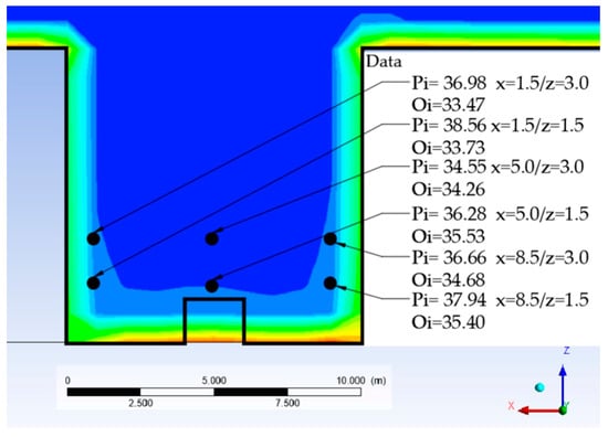
Figure 5.
Simulation section comparing simulated data (Pi) and field measurements (0i).
The Pi values were the six lines average in their different locations, at the height of 1.5 and 3.0 meters on the right sidewalk, in the middle of the street, and on the left sidewalk, as were the values for Oi, designated to the same height and distance.
The results of PMARE (%) in different positions are shown in Table 3. As shown in Figure 5, the values with the greatest difference between the simulation and the field are those located in the position X = 5.0 and Z = 1.5, because it is found above the vehicles, with the lowest value being PMARE 15.91, meaning fair.
Table 3.
Final values of PMARE for validation. PMARE rating for model validation is described in the following ranges: 0–5% is excellent, 5–10% very good; 10–15% good; 15–20% fair; 20–25% moderate; >25% is unsatisfactory.
3. Results
The final values of the simulations are noted in Table 4, expressing the mean TWA temperature (°C) of the 108 cases used for discussion and conclusions. The value represents the mean of the 900 air temperature data, divided into nine lines with one data every m along the idealized urban canyon (100 m). Within the data, it can be observed that the N–S canyons present higher temperature values because the west façade has a direct solar radiation of 1:00 p.m., in order to adapt to the measurement schedule of the case study. This due to the fact that in E–W orientation points closer to the façade facing east present higher temperatures in the morning; it also points closer to the façade facing west present higher temperatures in the afternoon, thus modifying the average values according to Grajeda et al. [36].
Table 4.
Modeled data with wind speed variations vs street orientation for each aspect-ratio [AR]. Values in °C.
3.1. Analysis in Relation to the Number of Vehicles
Based on the data in Table 4, Figure 6 is obtained, where the increase in °C is observed when including 10 or 20 vehicle units based on the urban canyons with zero cars. The four charts are divided by the two geographic orientations and width of the streets. A linear increase was observed in the canyon oriented to the N–S with a width of 10m, with an R2 = 0.90; the unfavorable case is in a canyon with the same width but with an E–W orientation.
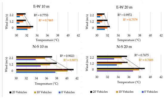
Figure 6.
The behavior of different urban canyons, in relation to the increase in the number of vehicles.
3.2. Analysis in Relation to Wind Speed
Table 5 compares the thermal behavior of TWA when the wind is parallel to the street (channeling effect) and has a speed of 1.2 and 2.2 m/s. It is concluded that the canyons with E–W orientation decrease from 1 to 2 °C, while those oriented N–S manage to decrease up to 3.8 °C, in relation to the canyons with a wind speed of 0.0 m/s.
Table 5.
Average reduction of temperature according to the mean wind speed for each orientation. Values in °C.
3.3. Analysis in Relation to the Orientation
Another important factor in the studies of urban canyons is the orientation, from which two dependent variables can be identified, shadow projection and wind behavior. The orientation, density, and aspect ratios of the canyon define the solar path, thus determining the time and angle of incidence of incoming solar radiation and increasing surface temperature, according to the amount of direct sunlight they receive [17].
Table 6 illustrates the TWA pattern in percentage, comparing the canyons with north-south orientation with the east-west ones as a base. The highest increases are in the narrowest canyons (10 m). The most significant difference is at the 20-vehicle canyon with 1.2 m/s wind speed, since the 10 m street presents a reduction of 19.4%; meanwhile, the 20 m street shows an 11.8% reduction, thus achieving a difference close to 8% between them.
Table 6.
Mean percentage of TWA increase in north–south canyons, compared with east–west canyons as a base.
Figure 7 identifies the behavior of TWA, where the highest ranges are north–south, with emphasis on the 10 m wide canyons, mainly in the 10/5, where the range goes from 33.8 (zero vehicles and wind speed of 2.2 m/s) to 41.7 °C (10 vehicles and 0.0 m/s wind speed), thus achieving a difference of almost 8 °C.
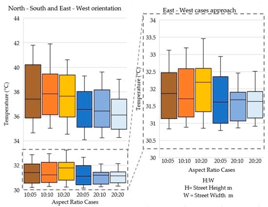
Figure 7.
Average percentage increase in north–south and east–west canyons.
4. Discussion and Conclusions
Field value measurements and those validated from the simulations were presented and contrasted against the QF database with diurnal and seasonal profiles generated by Sailor et al. [26] for a total of 61 US cities, sorted by cold and warm winters and introducing an extrapolation and statistical method of energy consumption.
From the results presented by Sailors [26] on QF and QFV, only the cities with warm winters were selected as our case study, and the percentage of the relative contribution of the QFV component that the authors calculated by averaging all cities per month.
Figure 8 shows the values used in the radiation equation to obtain the QFV in W m−2 of the TWA values obtained in the field measurements and simulation of this work, thus considering an emissivity of 0.55 (average of construction materials and vehicular auto body), i.e., a defined area of 1 m2 and σ = 5.67 × 10⁻⁸ W m−2 K−1. The values of TLOWER, in the case of field measurements, are the official temperatures of the meteorological center of the city; in the simulation, it is the value of the TWA of the homonymous urban canyon with zero vehicular units.
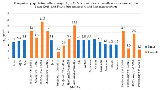
Figure 8.
Comparison of mean monthly QFV values for [26] versus the simulated (SIM) and field-measured (FM) TWA.
With the data in Figure 7 and Figure 8, in Figure 8 the average QFV values of [26], and those of this research are compared.
Field measurements were analyzed (Figure 8) in the warm period (May). An increase of 4 W m−2 was observed at the height of 1.5 m and 2.0 W m−2 at the height of 3.0 m, in relation to the data reported by Sailor et al. [26].
The simulations set in the month of June, in the warm period, with E–W orientation, are below the average for American cities; alternately, the simulations with N–S orientation showed an increase of 10 units equal to the value determined for these cities, but it was doubled (10.2 W m−2) with 20 units, that is, with a full capacity for a 100 m long urban canyon. The values in the field measurements in the month of February (semi-warm period) at the height of 1.5 m rose from 8.5 to 7.6 W m−2 (double) but were equal to the height of 3.0 m with the values of Sailor et al. [26].
Therefore, we can conclude that, at the height of 3.0 m, values were similar, and the influence of QFV, by means of the statistical estimation, did not reflect its intensity at 1.5 m height, where pedestrian movement takes place.
Regarding wind speed, researchers have determined it as an effective strategy to eliminate the UHI by calculating thresholds and limits according to several variables. For example, according to their extension, cities such as Kwangmyung (Korea), Kimagaya (Japan), Reading (England), and Hamilton (Canada) require 4.6, 5, 4–7, and 6–8 m/s to avoid the UHI, respectively [11,51], for cities with large populations. Kolokotroni and Giridharan [52] reported that London (England, population 8,500,000) required a value of 12 m/s, and Reading (England, 120,000) required values between 4 and 7 m/s.
A study that supports our findings related to the power of convection to mitigate heat flow in the urban canyon was conducted in Seoul (South Korea), supported by 54 automatic weather stations. It was evaluated that, in clear skies, the effect of the wind in the high peaks of UHI increased the wind speed results by 0.5 m/s, on average; with a decrease of 0.2 ◦C in UHI, compared to our results (Table 5), it was observed that the trend was mainly achieved in the canyons with N–S orientation (Figure 7), where reductions oscillated between 0.74, 0.52, and 0.49, respectively.
The aim of this research was to determine the weighing of one of the main factors of the formation of the UHI: vehicular anthropogenic heat (QHV), which directly affects the microclimatic variables, such as mean radiative temperature, dry bulb temperature, and relative humidity, presented in urban canyons or streets, whose effects are just a part of the thermal perception by the population’s thermal comfort.
It is concluded from the analyses of the temperature averages in the canyons that:
- The north–south orientation of the canyon (facades towards east–west) are those that represent the highest elevation in the thermal profile, since the solar path is perpendicular to the studied transect, thus causing both the horizontal area (street) and vertical area (east and west façades) to be affected by solar radiation, instead of just the horizontal area [36].
- Wind speed is a determining factor in calculating the internal temperature of the urban canyon because, in conditions of 0 m/s, temperature values are higher, although the difference in TWA offered between the speeds 1.2 and 2.2 m/s were not relevant for the streets with east–west orientation, as can be seen in Figure 6.
- The number of cars in the case studies (10 and 20 units) did not affect the decrease in temperature with wind speed at 1.2 m/s, where the E–W orientation decreased mostly by 1.5 °C and N–S-oriented lane decreased within a range of 3.3 to 4.6 °C.
- The increase in temperature inside the canyon is progressive with the increase in vehicles; however, in E–W canyons, it was proportional; that is, for every ten cars, it increased by 0.5 °C more. However, in N–S canyons, the increase was 1.6 °C; adding ten more units, it was 1.2 °C, which was, in this case, not proportional.
Given the complexity of simulating UHI in the ANSYS software, it is recommended that:
- (a)
- The domain (air volume) consistently exceeded twice the height of the highest urban element to avoid turbulence at the canopy level;
- (b)
- The mesh must adapt to the geometry of the domain, in this case tetrahedral, and have spatial treatment on smaller surfaces, such as vehicle volumes, if more precise data are required;
- (c)
- Perform a mesh sensitivity study to save simulation resources;
- (d)
- Determine the properties of materials and how they intervene in thermal and radiation processes;
- (e)
- Concerning the proposed radiation model (S2S), consider that the static simulation data represent the maximum values that can be obtained from the assigned conditions;
- (f)
- Using a realizable k-epsilon as a turbulence model is advisable because it considers pressure gradients between the walls to avoid calculation errors.
The data generated here allows for redirecting and reflecting on urban public policies, in order to seek strategies that allow for the reduction of outdoor thermal sensation for user comfort and distribution of the TWA gradient on the facades of buildings by considering the impact of planning on the dimensions of the streets and changes in the construction permit guidelines, in order to determine urban canyon heights as a function of the vehicular stream and design equipment in facades for heat gradient reduction (such as vegetation on the sidewalks or placed directly over facades) and adequate urban mobility to regulate vehicular flow.
Passive techniques should be considered, especially for N–S-oriented canyons, and avoid narrow configurations. These techniques can be: to determine a maximum vehicle capacity; to generate a constant flow or vehicular mobility; to close street circulation in overtheated hours; and, to raise awareness among users; reach a consensus so that the information is horizontally distributed and does not lead to traffic jams, which, in turn, leads to the problems that have been identified, calculated, and simulated in this work, as well as considering the constructive elements that help in heat dissipation and increase of wind turbulence.
The research encourages the subsequent analysis of mitigation techniques, such as controlled vehicular flow, through a limited or restricted number of vehicles per time unit or even temporary street closures, as well as considerations for roof design. If horizontal shading elements are to be considered, it is necessary to observe that, in addition to mitigating the radiation on pedestrians, it must allow the expulsion of heat and humidity generated by the engine combustion of vehicles.
Future research should focus on the mean radiant temperature and its modification due QFV in the thermal environment, as well as weighing it on the thermal perception of humans. Additionally, further analysis regarding different variables, such as wind speed, urban canyon ratio, and orientation, should be performed. Finally, another proposal worth investigating must be the intersection of the urban canyon and geometric form, in order to release heat flux from the buildings.
As the literature and this work have mentioned, vehicular anthropogenic heat presents many variables for its analysis and numerous considerations for data collection in the field. This manuscript and its methodology presented aids for the simplification of the number of data to obtain QFV.
Author Contributions
R.M.G.-R.: conceptualization, methodology, formal analysis, investigation, and writing—original draft preparation. E.M.A.-G.: conceptualization, formal analysis, writing—review and editing, and supervision. C.E.-D.P.: software, validation, and visualization. C.J.E.-L.: methodology, formal analysis, writing—original draft preparation, and supervision. C.S.-S.: formal analysis and writing—original draft preparation. W.M.-M.: resources and writing—review and editing. M.M.-O.: investigation, resources, and writing—review and editing. A.C.-M.: writing—review and editing and visualization. All authors have read and agreed to the published version of the manuscript.
Funding
This research received no external funding.
Institutional Review Board Statement
Not applicable.
Informed Consent Statement
Not applicable.
Acknowledgments
The first author would like to acknowledge the minister of science and technology from Mexico (CONACyT in Spanish) for the grant during her studies.
Conflicts of Interest
The authors declare no conflict of interest.
References
- United Nations. World Urbanization Prospects: The 2014 Revision, Highlights (ST/ESA/SER.A/352); United Nations: New York, NY, USA, 2014. [Google Scholar]
- He, B.J.; Wang, J.; Liu, H.; Ulpiani, G. Localized synergies between heat waves and urban heat islands: Implications on human thermal comfort and urban heat management. Environ. Res. 2021, 193, 110584. [Google Scholar] [CrossRef] [PubMed]
- He, B.J.; Ding, L.; Prasad, D. Wind-sensitive urban planning and design: Precinct ventilation performance and its potential for local warming mitigation in an open midrise gridiron precinct. J. Build. Eng. 2020, 29, 101145. [Google Scholar] [CrossRef]
- Ruth, M.; Baklanov, A. Urban climate science, planning, policy and investment challenges. Urban Clim. 2012, 1, 1–3. [Google Scholar] [CrossRef]
- Li, H.; Zhou, Y.; Li, X.; Meng, L.; Wang, X.; Wu, S.; Sodoudi, S. A new method to quantify surface urban heat island intensity. Sci. Total Environ. 2018, 624, 262–272. [Google Scholar] [CrossRef] [PubMed]
- Ramakreshnan, L.; Aghamohammadi, N.; Fong, C.S.; Ghaffarianhoseini, A.; Ghaffarianhoseini, A.; Wong, L.P.; Hassan, N.; Sulaiman, N.M. A critical review of Urban Heat Island phenomenon in the context of Greater Kuala Lumpur, Malaysia. Sustain. Cities Soc. 2018, 39, 99–113. [Google Scholar] [CrossRef]
- Strømann-Andersen, J.; Sattrup, P.A. The urban canyon and building energy use: Urban density versus daylight and passive solar gains. Energy Build. 2011, 43, 2011–2020. [Google Scholar] [CrossRef]
- Santamouris, M.; Asimakopoulos, D.N.; Assimakopoulos, V.D.; Chrisomallidou, N.; Klisikas, N.; Mangold, D.; Michel, P.; Tsangrassoulis, A. Energy and Climate in the Urban Built Environment; Routledge: Oxfordshire, UK, 2011; ISBN 9781873936900. [Google Scholar]
- Lemos, L.d.O.; Oscar Júnior, A.C.; Mendonça, F. Urban canyon in the CBD of Rio de Janeiro (Brazil): Thermal profile of avenida rio branco during summer. Atmosphere 2022, 13, 27. [Google Scholar] [CrossRef]
- Nikolopoulou, M.; Steemers, K. Thermal comfort and psychological adaptation as a guide for designing urban spaces. Energy Build. 2003, 35, 95–101. [Google Scholar] [CrossRef]
- He, B.-J. Potentials of meteorological characteristics and synoptic conditions to mitigate urban heat island effects. Urban Clim. 2018, 24, 26–33. [Google Scholar] [CrossRef]
- Ngarambe, J.; Oh, J.W.; Su, M.A.; Santamouris, M.; Yun, G.Y. Influences of wind speed, sky conditions, land use and land cover characteristics on the magnitude of the urban heat island in Seoul: An exploratory analysis. Sustain. Cities Soc. 2021, 71, 102953. [Google Scholar] [CrossRef]
- Li, D.; Bou-Zeid, E. Synergistic Interactions between Urban Heat Islands and Heat Waves: The Impact in Cities Is Larger than the Sum of Its Parts. J. Appl. Meteorol. Climatol. 2013, 52, 2051–2064. [Google Scholar] [CrossRef] [Green Version]
- Oke, T. The urban energy balance. Prog. Phys. Geogr. Earth Environ. 1988, 12, 471–508. [Google Scholar] [CrossRef]
- Sailor, D.J. A review of methods for estimating anthropogenic heat and moisture emissions in the urban environment. Int. J. Climatol. 2011, 31, 189–199. [Google Scholar] [CrossRef]
- Mirzaei, P.A. Recent challenges in modeling of urban heat island. Sustain. Cities Soc. 2015, 19, 200–206. [Google Scholar] [CrossRef] [Green Version]
- Bottillo, S.; De Lieto Vollaro, A.; Galli, G.; Vallati, A. Fluid dynamic and heat transfer parameters in an urban canyon. Sol. Energy 2014, 99, 1–10. [Google Scholar] [CrossRef]
- Gagliano, A.; Nocera, F.; Aneli, S. Computational Fluid Dynamics Analysis for Evaluating the Urban Heat Island Effects. Energy Procedia 2017, 134, 508–517. [Google Scholar] [CrossRef]
- Grajeda-Rosado, R.M.; Alonso-Guzman, E.M.; Esparza-Lopez, C.J.; Escobar-Del Pozo, C. Simulación del comportamiento térmico en exteriores urbanos correlacionando las variables de calor antropogénico vehicular y orientación. Rev. Simulación Lab. 2019, 6, 19–33. [Google Scholar] [CrossRef]
- Grajeda-Rosado, R.M.; Alonso-Guzman, E.M.; Martínez Molina, W.; Bedolla Arroyo, J.A.; Esparza-Lopez, C.J.; Chávez García, H.L. Thermal Analysis of the Urban Canyon Based on the Variables: Orientation, Wind and Vehicular Anthropogenic Heat. IOP Conf. Ser. Mater. Sci. Eng. 2020, 811, 012044. [Google Scholar] [CrossRef]
- Jin, K.; Wang, F.; Wang, S. Assessing the spatiotemporal variation in anthropogenic heat and its impact on the surface thermal environment over global land areas. Sustain. Cities Soc. 2020, 63, 102488. [Google Scholar] [CrossRef]
- Takahashi, K.; Yoshida, H.; Tanaka, Y.; Aotake, N.; Wang, F. Measurement of thermal environment in Kyoto city and its prediction by CFD simulation. Energy Build. 2004, 36, 771–779. [Google Scholar] [CrossRef]
- He, C.; Zhou, L.; Yao, Y.; Ma, W.; Kinney, P.L. Estimating spatial effects of anthropogenic heat emissions upon the urban thermal environment in an urban agglomeration area in East China. Sustain. Cities Soc. 2020, 57, 102046. [Google Scholar] [CrossRef]
- Holt, T.; Pullen, J. Urban canopy modeling of the New York City metropolitan Area: A comparison and validation of single- and multilayer parameterizations. Mon. Weather Rev. 2007, 135, 1906–1930. [Google Scholar] [CrossRef] [Green Version]
- Lin, C.Y.; Chen, F.; Huang, J.C.; Chen, W.C.; Liou, Y.A.; Chen, W.N.; Liu, S.C. Urban heat island effect and its impact on boundary layer development and land-sea circulation over northern Taiwan. Atmos. Environ. 2008, 42, 5635–5649. [Google Scholar] [CrossRef]
- Sailor, D.J.; Georgescu, M.; Milne, J.M.; Hart, M.A. Development of a national anthropogenic heating database with an extrapolation for international cities. Atmos. Environ. 2015, 118, 7–18. [Google Scholar] [CrossRef] [Green Version]
- Chow, W.T.L.; Salamanca, F.; Georgescu, M.; Mahalov, A.; Milne, J.M.; Ruddell, B.L. A multi-method and multi-scale approach for estimating city-wide anthropogenic heat fluxes. Atmos. Environ. 2014, 99, 64–76. [Google Scholar] [CrossRef] [Green Version]
- Sailor, D.J.; Lu, L. A top-down methodology for developing diurnal and seasonal anthropogenic heating profiles for urban areas. Atmos. Environ. 2004, 38, 2737–2748. [Google Scholar] [CrossRef]
- Sun, R.; Wang, Y.; Chen, L. A distributed model for quantifying temporal-spatial patterns of anthropogenic heat based on energy consumption. J. Clean. Prod. 2018, 170, 601–609. [Google Scholar] [CrossRef]
- Smith, C.; Lindley, S.; Levermore, G. Estimating spatial and temporal patterns of urban anthropogenic heat fluxes for UK cities: The case of Manchester. Theor. Appl. Climatol. 2009, 98, 19–35. [Google Scholar] [CrossRef]
- Quah, A.K.L.; Roth, M. Diurnal and weekly variation of anthropogenic heat emissions in a tropical city, Singapore. Atmos. Environ. 2012, 46, 92–103. [Google Scholar] [CrossRef]
- Santamouris, M. Urban warming and mitigation. In Urban Climate Mitigation Techn; Routledge: Oxfordshire, UK, 2016. [Google Scholar]
- Dirección de obras públicas y desarrollo social Plan Distrito Centro; Veracruz, 2019. Available online: https://distritocentro.veracruzmunicipio.gob.mx/index.html (accessed on 22 April 2019).
- Velasco Toro, J.; Félix Báez, J. Ensayos Sobre la Cultura de Veracruz: Arqueología, Etnología, Cultura Popular, Educación, Historiografía, Arquitectura, Plástica, Literatura, Ciencias Naturales, 2nd ed.; Universidad Veracruzana: Veracruz, Mexico, 2000. [Google Scholar]
- Kottek, M.; Grieser, J.; Beck, C.; Rudolf, B.; Rubel, F. World map of the Köppen-Geiger climate classification updated. Meteorol. Z. 2006, 15, 259–263. [Google Scholar] [CrossRef]
- Grajeda Rosado, R.M.; Alonso Guzman, E.M.; Esparza López, C.J. Vehicular anthropogenic heat in the physical parameters of an urban canyon for warm humid climate. In PLEA 2018—Smart and Healthy within the Two-Degree Limit: Proceedings of the 34th International Conference on Passive and Low Energy Architecture; 2018; Volume 1, Available online: http://web5.arch.cuhk.edu.hk/server1/staff1/edward/www/plea2018/home.html (accessed on 14 May 2019).
- Tomlinson, C.J.; Chapman, L.; Thornes, J.E.; Baker, C. Remote sensing land surface temperature for meteorology and climatology: A review. Meteorol. Appl. 2011, 18, 296–306. [Google Scholar] [CrossRef] [Green Version]
- Anderson, M.C.; Allen, R.G.; Morse, A.; Kustas, W.P. Use of Landsat thermal imagery in monitoring evapotranspiration and managing water resources. Remote Sens. Environ. 2012, 122, 50–65. [Google Scholar] [CrossRef]
- Mia, M.B.; Bromley, C.J.; Fujimitsu, Y. Monitoring heat flux using Landsat TM/ETM+ thermal infrared data—A case study at Karapiti (Craters of the Moon’) thermal area, New Zealand. J. Volcanol. Geotherm. Res. 2012, 235–236, 1–10. [Google Scholar] [CrossRef]
- Rosado, R.M.G.; Guzmán, E.M.A.; Lopez, C.J.E.; Molina, W.M.; García, H.L.C.; Yedra, E.L. Mapping the LST (Land Surface Temperature) with Satellite Information and Software ArcGis. IOP Conf. Ser. Mater. Sci. Eng. 2020, 811, 012045. [Google Scholar] [CrossRef]
- INEGI, Instituto Nacional de Geografía, Estadística e Informática. Inventario Nacional de Vivienda. Available online: http://www.beta.inegi.org.mx/app/mapa/INV/Default.aspx?ll=19.185135,-96.14908000000003&z=13 (accessed on 6 June 2019).
- Instituto Nacional de Ecología y Cambio Climático (INECC); Dirección de Investigación sobre la Contaminación Urbana y Regional (DGICUR); Dirección de Investigación sobre la Calidad del Aire (DICA). Estudio de Emisiones y Actividad Vehícular en el Puerto de Veracruz, Veracruz; INECC; SEMARNAT: Ciudad de México, Mexico, 2012.
- World Meteorological Organzation. Guía de Instrumentos y Métodos de Observación Meteorológicos; World Meteorological Organzation: Geneva, Switzerland, 2014. [Google Scholar]
- ANSYS, Inc. ANSYS Fluent Theory Guide; Ansys: Canonsburg, PA, USA, 2013. [Google Scholar]
- Nazarian, N.; Kleissl, J. CFD simulation of an idealized urban environment: Thermal effects of geometrical characteristics and surface materials. Urban Clim. 2015, 12, 141–159. [Google Scholar] [CrossRef]
- Cascetta, F.; Musto, M. Assessment of thermal comfort in a car cabin with sky-roof. Proc. Inst. Mech. Eng. Part D J. Automob. Eng. 2007, 221, 1251–1258. [Google Scholar] [CrossRef]
- Cengel, Y.A.; Ghajar, A.J. Heat and Mass Transfer, 4th ed.; Mc Graw Hill; Springer: Barcelona, Spain, 2011. [Google Scholar]
- Yuan, C.; Adelia, A.S.; Mei, S.; He, W.; Li, X.-X.; Norford, L. Mitigating intensity of urban heat island by better understanding on urban morphology and anthropogenic heat dispersion. Build. Environ. 2020, 176, 106876. [Google Scholar] [CrossRef]
- Aghamolaei, R.; Fallahpour, M.; Mirzaei, P.A. Tempo-spatial thermal comfort analysis of urban heat island with coupling of CFD and building energy simulation. Energy Build. 2021, 251, 111317. [Google Scholar] [CrossRef]
- Ali, M.H.; Abustan, I. A new novel index for evaluating model performance. J. Nat. Resour. Dev. 2014, 4, 1–9. [Google Scholar] [CrossRef]
- Park, H.S. Features of the heat island in Seoul and its surrounding cities. Atmos. Environ. 1986, 20, 1859–1866. [Google Scholar] [CrossRef]
- Kolokotroni, M.; Giridharan, R. Urban heat island intensity in London: An investigation of the impact of physical characteristics on changes in outdoor air temperature during summer. Sol. Energy 2008, 82, 986–998. [Google Scholar] [CrossRef] [Green Version]
Publisher’s Note: MDPI stays neutral with regard to jurisdictional claims in published maps and institutional affiliations. |
© 2022 by the authors. Licensee MDPI, Basel, Switzerland. This article is an open access article distributed under the terms and conditions of the Creative Commons Attribution (CC BY) license (https://creativecommons.org/licenses/by/4.0/).