Abstract
Aircraft-Induced Clouds (AICs), colloquially called contrails, form from the emission of soot from jet engines during cruise flight in favorable atmospheric conditions. AICs absorb, scatter, and reflect shortwave and longwave radiation. This radiative transfer has a cooling effect during the day; however, the night experiences an overwhelming warming effect, which leads to an overall warming effect on Earth, contributing to anthropogenically propelled climate change. Reducing AICs significantly mitigates aviation’s contribution to climate change by reducing the disruption in Earth’s radiation budget. Researchers have proposed AIC Abatement Programs (AAPs) to increase cruise flight levels without additional fuel burn. In order to effectively implement AAPs, it is crucial to be able to accurately identify AICs from publicly available aerial and satellite imagery. This study aims at the identification of AICs from hyperspectral imagery to help the effective implementation of an AAP and to mitigate climate change. This paper describes a method for the hyperspectral analysis of aerial images in order to accurately identify AICs through a case study based in West Virginia. The results show that both the Adaptive Coherence Estimator and the Matched Filter algorithms based on unique in-scene spectra were successful in the isolation of the AICs from other cloud types and the background. It is found that AICs can be identified with 84% confidence in this case study. The method, a case study, and future works are provided.
1. Introduction
An atmosphere conducive to the formation of AICs meets the Schmidt–Appleman criteria (≤−41.1 °C and ≥100% relative humidity) and has soot from jet engine emissions serving as cloud condensation nuclei. The atmospheric water vapor bonds to the soot particles and creates ice crystals, which may grow and replicate, forming cirrus-like anthropogenic clouds. AICs absorb, scatter, and reflect approximately 33% of longwave thermal radiation back to Earth [1]. Without AIC interference in Earth’s natural radiation budget, this radiation would be transmitted back to space, barring any interaction with natural clouds. The result is an increase in Earth’s average temperature [1]. During daytime, as a function of the solar zenith, AICs can also provide a cooling effect by reflecting approximately 23% of the incoming shortwave solar radiation back to space. It is crucial to note that AICs have a net warming effect of approximately 10%, calculated by subtracting the cooling effect from the warming effect. The lifetime of greenhouse gases such as CO2 in the troposphere is significantly longer (20–40 years) than that of AICs. An atmosphere clear of AICs may immediately reap the benefits, which indicates the climatic benefits of AAPs [2].
In the National Airspace System (NAS), AICs occur in only 15% of daily flights on average, with a maximum value of 34% of daily flights [3]. The location of an AIC is a function of atmospheric conditions, known as Ice Super Saturated Regions (ISSRs), which occur mostly over the west coast, and the southeastern and mid-Atlantic regions of the United States. After several minutes and especially several hours, the shape of an AIC transitions to a natural cirrus cloud-like appearance, called a contrail cirrus, due to the high winds of the jet streams at the altitude of the AIC. The loss of AIC linearity decreases confidence in the validation of AICs from satellite imagery. A temporal limitation is often imposed in order to increase confidence. A key objective in the remote sensing of AICs is the differentiation between a natural cirrus and a contrail cirrus. The literature shows optical and microphysical differences between a cirrus and an AIC pertaining to crystal shape (habit), particle size distribution, backscattering coefficients, and linear depolarization ratios [4,5,6,7,8]. In addition to these differences, hyperspectral nuances increase the confidence of a positive identification of AICs from hyperspectral imagery.
This paper describes a method for the hyperspectral analysis of aerial images in order to identify AICs. The method includes five steps: the elimination of bad bands, the identification and overlay of primary regions of interest, the creation of a spectral library based on in-scene spectra, running of algorithms with in-scene spectra on the image, and the isolation of clouds with histogram stretching and color table manipulation.
The process is demonstrated with an aerial image from NASA AVIRIS (Airborne Visible/Infrared Imaging Spectrometer) Classic flight f090714t01p00r08, Fernow Experimental Forest, Monongahela National Forest, West Virginia. The first set of two digits of the flight number indicates the last two digits of the year of the flight, the second set of two digits indicates the month, and the third set of two digits indicates the day. The last nine characters are unique to the specific flight line as AVIRIS flights are often conducted in a series of several proximal sites. The location of the case study is Fernow Experimental Forest, Monongahela National Forest, West Virginia, on 14 July 2009, at 15:02 UTC (11:02 EST), and the spatial resolution measured by pixel size is 16 m. The AVIRIS flight altitude is estimated to be approximately 18,288 m above Mean Sea Level (MSL), while the flight that generated the AIC is estimated to be between 9144 and 12,192 m above MSL. Images were processed using the Adaptive Coherence Estimator (ACE) and Matched Filter (MF) algorithms. Image preprocessing and analysis were completed with the L3 Harris ENVI Classic version 5.6.1.
This paper is organized as follows: Section 2 describes the overall process for generating AIC inventories from hyperspectral images and the special role of a spectral analysis. Section 3 describes the methods for spectral analysis. Section 4 provides the results of the spectral analysis of the NASA Airborne Visible/Infrared Imaging Spectrometer (AVIRIS) hyperspectral image [9]. Section 5 discusses the implications of these results and future work.
2. Data and Methodology
The main goal of AIC Abatement Programs is to use AIC inventories to mitigate the presence of AICs and thus to lower the contribution of aviation to global warming [2]. AIC inventories should be updated at regular intervals throughout the National Airspace System (NAS). The inventory ought to be based on the positive validation of AICs from remotely sensed imagery. A high spatial resolution is crucial for a positive identification and has led to the selection of hyperspectral imagery data for this case study. The current literature [10,11,12,13,14] shows significant spatial and spectral resolution constraints in machine learning for AIC identification, thereby leading to a low confidence. Specific domain skill gaps discovered by a literature review include physical tropospheric patterns, hyperspectral remote sensing, and airline threaded flight tracks as gaps.
Current methods for the AIC inventory of the NAS involve the remote sensing of hyperspectral aerial imagery and threaded airline flight tracks overlaid with Ice Super Saturated Regions (ISSRs) identified by processing of the Schmidt–Appleman criteria data [15]. Based on the Schmidt–Appleman criteria, AICs are assumed to be persistent (non-dissipating). This method is most direct. Existing methods use satellite imagery and Machine Learning (ML) in order to identify AICs. To train and validate the ML model, the satellite images with and without AICs must be semantically annotated after a visual separation of AICs and natural clouds. Satellite imagery, however, has lower spatial and spectral resolutions. The spatial resolution of the AVIRIS image used in this study is 16 m whereas the typical satellite imagery resolution is around 1 km. The spectral resolution of the AVIRIS image used in this study is 224 bands, whereas the typical satellite spectral resolution is around 16 bands. These limitations in resolution lead to a low confidence of AIC detection from satellite imagery and high rates of false positives and false negatives [10,11,12,13,14]. These limitations in spectral and spatial resolutions serve as deciding factors in the use of hyperspectral data for the methodology proposed in this paper.
Figure 1 outlines the current research scope and plan towards improving the reliability of AIC identification from remotely sensed imagery. The scope involves three primary methods of AIC verification: (1) hyperspectral remote sensing; (2) atmospheric physics to include the coexistence with ISSRs, Schmidt–Appleman criteria, and jet stream involvement; and (3) coexistence with airline flight threaded tracks. These three methods are color-coded in Figure 1 in tan, blue, and gray, respectively.
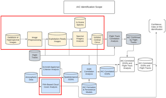
Figure 1.
AIC Identification Scope Block Diagram.
The upper row from left to right shows the conversion of hyperspectral images into exploitation-ready images for the isolation of AICs. This is accomplished using in-scene spectra and spectral imagery analysis (spectral mapping algorithms).
The lower row uses atmospheric data and flight track data, along with AIC formation and persistence models in order to predict the presence of AICs in the image. The Federal Aviation Administration (FAA) has quantitative definitions of cloud coverage determined from ground sensors at airport weather stations, as outlined in Table 1 from the FAA Aeronautical Information Manual (AIM) 7-1-29 b. 1, e. The celestial dome projected from the sensor divides the sky into octas. Each octal that has clouds is added up and categorized into five classes. Clear skies indicate 0 cloud coverage. A few clouds indicate cloud coverage between 0 and 2 octas. Scattered clouds indicate cloud coverage between 3 and 4 octas. Broken clouds indicate cloud coverage between 5 and 7 octas. Lastly, overcast skies indicate 100% cloud coverage. The last two categories are considered ceilings. [15] The method used in this research is adapted and inverted from a domed bottom-up view to a flat top-down view in order to match the sensor view from the airplane. A pixel count is to be completed in ENVI and the percentage of pixels, representative of cloud cover, will be incorporated into the confidence index in lieu of the octal system. There exists an inverse relationship between cloud cover and confidence as it is easier to identify AICs with fewer clouds in the vicinity obscuring the view. In this scenario, confirmation with atmospheric physical analysis and airline flight track data is ideal.

Table 1.
FAA quantitative definitions of cloud coverage.
The results of the remote sensing and the atmospheric physics analysis are combined, resulting in a confidence level capturing the methods’ accuracy. This study focuses on the items outlined in red boxes in Figure 1 to include all of the hyperspectral remote sensing steps.
Hyperspectral imagery analysis is a high-precision method of obtaining radiation data and spectral signatures without physical contact with the object or medium of interest. Spectral signatures are often the response of radiation to some chemical structures and physical properties of the objects being observed. Radiation and Earth’s atmosphere interact by means of absorption, scattering, extinction, and attenuation of radiation. Spectral scientists have classified several bands of the electromagnetic spectrum with similar characteristics such as the visible band and the infrared band. Hyperspectral measurements have hundreds of small bands, while multispectral measurements have several large bands. Hyperspectral sensors such as AVIRIS provide higher rates of contiguity, resolution, and precision. AVIRIS Classic is used in this analysis and offers 224 continuous bands between 0.38 µm and 2.510 µm. The spectrum of each pixel in the image is matched to the value range defined by the user in the histogram after the algorithm application is determined to be either part of the AIC.
The method for the hyperspectral analysis of AICs takes a raw NASA AVIRIS hypercube, preprocesses it, and applies the spectral analysis in order to isolate the AIC (Figure 2). This is a 5-step process:
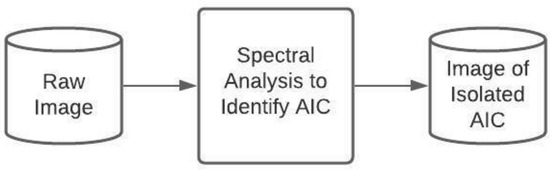
Figure 2.
Abridged Method for Hyperspectral Analysis of AIC.
- Eliminate Bad Bands
- Create and Overlay Regions of Interest
- Create Spectral Library based on In-Scene Spectra
- Run Algorithms (ACE, MF) with In-Scene Spectra on Image
- Isolate AIC with Histogram Stretching and Color Table Manipulation
Image preprocessing and analysis were completed with the Imagery Analysis Remote Sensing Tool, L3 Harris ENVI Classic version 5.6.1.
Step 1: Eliminate Bad Bands
NASA AVIRIS Classic allows for imagery analysis in a maximum of 224 bands. Using the band animation tool, every band is visually inspected one by one in order to determine if it is bad (has noise). Those bad bands are then removed from the image header file within ENVI. For this image, preprocessing identified 107 bad bands. These were removed from the hypercube, thereby leaving 117 bands used for this analysis.
Step 2: Create and Overlay Regions of Interest
In this study, six Regions of Interest (ROIs) are established as outlined in Table 2, five of which are clouds: aircraft-induced, altostratus, stratus, cirrus, and cumulus. The last ROI covers the developed areas in the scene, which is an area that may be misinterpreted by algorithms for clouds due to its proximity to the cumulus clouds and its light color. The primary ROI is the AIC in the image.
Table 2.
Regions of interest.
The preparation for exploitation-ready imagery involved creating a library of in-scene Regions of Interest (ROI), whose spectral signatures are graphed in Figure 3 and Figure 4. Figure 3 shows the spectral signatures prior to the removal of bad bands, which are generally shown by the diagonal lines. In Figure 4, the diagonal lines are replaced with gaps. The removal of bad bands allows for an increased accuracy in reading this graph as well as an increased reliability of the algorithms. The primary region of interest is the AIC in the image, followed by other cloud types.
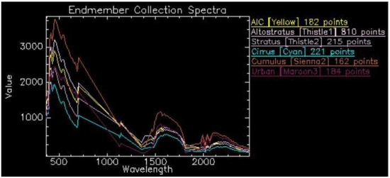
Figure 3.
ROI spectral signatures with bad bands for five cloud types and developed area.
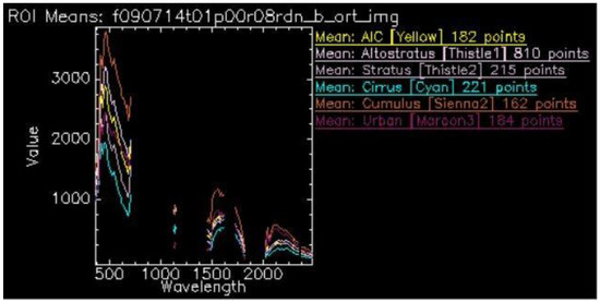
Figure 4.
ROI spectral signatures without bad bands for five cloud types and developed area.
Cirrus clouds, under which contrail cirrus clouds may be classified, tend to be mapped spectrally around 1.375 μm due to a strong atmospheric water vapor absorption [2,16]. Although this wavelength was included in the bad bands list in preprocessing and thus excluded from Figure 4, the spectral patterns between the atmospheric water vapor absorption and AIC radiance are consistent. It is important to note that Figure 4 shows the in-scene spectra from the case study prior to the partial atmospheric compensation, which is unique to the altitude of the AIC and the solar zenith angle.
Step 3: Create a Spectral Library Based on In-Scene Spectra
A spectral library is a collection of spectral patterns for different materials and is used to identify objects in the image. It is reflected as radiance or reflectance values across a fixed section of the electromagnetic spectrum. Spectrally similar substances have similar radiance levels across the electromagnetic spectrum. Figure 4 displays the layered spectra of the in-scene library adjusted for bad bands. In the visible range of the electromagnetic spectrum (0.4–0.7 µm), the ROIs are most similar. The lower extent of the AVIRIS wavelength range (380 nm) and the upper extent (2510 nm) are seen on the horizontal axis. Radiance is represented on the vertical axis. Radiance is directly measured by the AVIRIS sensor and uses the units Watt/(steradian·m2·nm).
At this time, there are no spectral libraries for clouds. This limitation does not allow for laboratory comparisons in research in the remote sensing of clouds, while they are more available in the remote sensing of Earth’s surface.
Step 4: Run Algorithms (ACE and MF) with In-Scene Spectra on the Images
The two algorithms used in this study are the ENVI Adaptive Coherence Estimator (ACE) and Matched Filter (MF). Both the ACE and MF assess composition (AICs, some AICs, or no AICs) on a pixel-by-pixel basis.
2.1. Adaptive Coherence Estimator (ACE)
ENVI ACE is a statistics-based pixel decomposition using the in-scene spectral library from Step 3. The algorithm determines the spectral composition percentage within pixels. It can be considered a cosine squared-normalized-matched filter with typically orthogonal eigenvectors. An exception to the orthogonal eigenvectors is singularity. Singularity is difficult to decompose in that it can create an issue of collinearity. Histogram values and near-target results have a direct relationship, like MF. The ACE formula for evaluating pixels in an image is expressed in Equation (1) [17].
where t is the reflectance value of the target pixel, μ represents the mean background noise, Γ represents the covariance matrix, and x is the source pixel from the ROI.
2.2. Matched Filter (MF)
The ENVI Matched Filter (MF) uses the in-scene spectral library from Step 3 in order to identify and isolate objects in the image. MF provides an output similar to ACE, however in eigenvector form. It typically works better than ACE in discarding non-target spectra. MF is a statistically based algorithm with an increased sensitivity to the target signal. Unfortunately, this characteristic has led to an elevated tendency for false positives. MF units are dimensionless real numbers between 0 and 1, inclusive. The MF formula for evaluating pixels in an image is expressed in Equation (2) [17].
where t is the reflectance value of the target pixel, μ represents the mean background noise, Γ represents the covariance matrix, and x is the source pixel from the ROI. The denominator is a non-square-rooted Mahalanobis distance.
Step 5: Isolate AICs with Histogram Stretching and Color Table Manipulations
Interactive histogram stretching, also known as input cropping, with boundaries towards higher values for ACE and MF adjusts the pixel brightness in response to the percentage value of the pixel. Histogram stretching is a user-defined linear expansion of sections of the original histogram. The intensity range occupies the full dynamic grayscale, as depicted by Equation (3). S is the user-defined pixel subset.
where r is function intensity, and L is the number of intensity levels, which is calculated by Equation (4) [18].
where k is an integer between 0 and bbp (bits by pixel). Histogram values in the user-defined range in Step 5 are included in the match where brightness is a result of pixel decomposition.
The last step is to change the scheme and to stretch the color tables. The color scheme was changed to black and white, where the AIC is shown as white, while everything else is shown as black, in the spectrally matched results of ACE and MF.
3. Results
The histogram for the ACE AIC is stretched to the range 0.009–0.785 (see Figure 5) and the histogram for the MF AIC is stretched to the range 0.095–2.374 (see Figure 6). Alongside the visual inspection of the AIC isolation in the image, the algorithm results within these quantified ranges are considered AICs. With both algorithms, the AIC was isolated from 100% of other cloud and surface types and maintained a textural nuance associated with the wake phase of AIC development. The final imagery results are shown in Figure 7. None of this texture was lost in the imagery due to the top-down view of the AVIRIS sensor or the high solar illumination that is often the case with larger clouds such as the cumulus. Despite ACE being more selective in pixel classification than MF, ACE yielded brighter results. None of the surrounding stratus clouds were mistaken by the algorithm for AICs, indicating a successful ROI selection and creation.
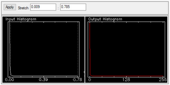
Figure 5.
ACE histogram stretched for AIC isolation.
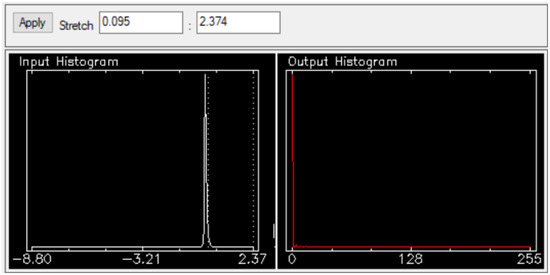
Figure 6.
MF histogram stretched for AIC isolation.
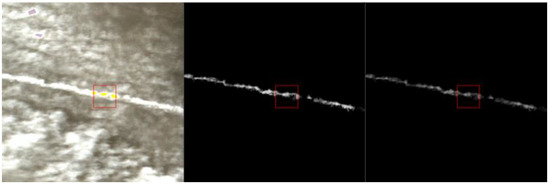
Figure 7.
True color image with ROIs, isolation of AIC with ACE, and isolation of AIC with MF results.
The images were processed using the Adaptive Coherence Estimator (ACE) and Matched Filter (MF). The main goal of this study is to use these algorithms in order to isolate AICs, specifically from other present cloud types such as the altostratus, stratus, and cirrus. The results in Figure 7 show three images in one display. The leftmost image in the display is the true color image in the red-green-blue (RGB) format where the bands are 29, 20, and 12, representing wavelengths 0.6381865 µm, 0.5503 µm, and 0.4724773 µm, respectively. Wavelengths with seven significant figures exemplify the higher quality of hyperspectral data over multispectral data. The ROIs are overlaid in the leftmost image, and their colors correspond to those shown in Figure 3 and Figure 4. The center image in the display shows the results of ACE in isolating the AIC. The rightmost image shows the results of MF in isolating the AIC. The red box in the center of each image in Figure 7 is of the same size and location in each image. The key findings in the results are the isolation of the AIC from the surrounding stratus clouds and the ground features.
4. Discussion
The AICs were successfully isolated from the rest of the contents of the imagery. AICs most closely resembled the altostratus clouds spectrally in this case study and their differentiation required additional histogram stretching. In order to accomplish this, some AIC pixels, likely with a lower optical depth, were excluded from the final results as they did not meet the threshold required to additionally exclude the altostratus clouds. The remaining results of the AIC are the majority and show promising results for the methodology, which are to be expanded through other hyperspectral images, including AICs. The AIC maintained a textural nuance associated with the wake phase of the AIC development. Despite ACE being more selective in pixel classification than MF, ACE yielded brighter results. None of the surrounding stratus clouds were mistaken by the algorithm for AICs, indicating the successful ROI selection and creation. Part of this success came from the uniform solar illumination and clean edges of this estimated relatively young AICs. Both algorithms were applied to all bands, excluding those from the bad bands list.
The AICs were entirely isolated, yielding a score of 100% in the confidence index; see Table 2. In order to estimate cloud coverage, the three cloud types present in the spatial subset of the case study were assigned bands for a false color composite; see Figure 8. The red band is assigned as AIC, the green band is assigned as altostratus clouds, and the blue band is assigned as stratus clouds. Following the FAA cloud coverage definitions from Table 1, it is estimated, based on the results from Figure 8, that local sky conditions were few (2/8 octas). Because of the inverse relationship between cloud coverage and the confidence of validation of the AIC from the image, this result is inverted from 2/8 to 6/8, which is represented as a percentage (75%). However, as seen in the red boxes in Figure 8, the AIC shadow (seen clearly in the left image) has been mistaken for a stratus cloud in the right image, slightly skewing the results. There is room for improvement here, which the authors take as a direction for further work.
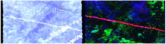
Figure 8.
Left image shows a false color image highlighting the AIC shadow on the ground. Right image shows a false color composite representing cloud coverage.
Given the age of this image, no atmospheric data (Schmidt–Appleman criteria) or airline threaded track records were found, which yielded a rating of 0 in the confidence index. Weights across all four confidence index parameters were initially equal at 25%; however, given such positive results in AIC isolation and cloud coverage, the Schmidt—Appleman criteria and threaded track weights are reduced from 25 to 2% and the AIC isolation and cloud coverage weights increased from 25 to 48%. It is with 84% confidence that the cloud identified in the case study is an AIC (Table 3).
Table 3.
Confidence index for the case study.
In addition to the improved accuracy in cloud shadow vs. cloud identification, future work in utilizing hyperspectral imagery for AIC detection and identification lies primarily in increasing the confidence index by overlaying isolated AICs with georeferenced threaded airline flight tracks, atmospheric data on the Schmidt–Appleman criteria, and jet stream patterns. There might be potential to quantify the optical depth from the algorithm output. Additional directions for further research include moving away from the octal system of cloud coverage, using the pixel count percentage of the total in the spatial subset, and defining the spatial subset distance from AICs. For additional analysis of spectral patterns, bandwidths known for their water vapor absorption, such as 1.38 μm, may be the focus for AIC isolation. This bandwidth is consistent with multispectral sensors and remote sensing analysis. The procedure developed in this study would benefit from machine learning techniques and can be implemented in the automated processing for different remote sensing systems such as MODIS data. These works are now in progress. Once the process can be automated and large amounts of data can be processed, the validation of the proposed methods should be performed with a larger dataset of images with more AICs, which could provide a statistical significance and a training model for automated processes of AIC identification. The case study here provides proof of this concept.
5. Conclusions
This paper describes a method for the hyperspectral analysis of remotely sensed aerial images in order to validate the presence of AICs. The method eliminates bad bands, identifies and overlays primary regions of interest, creates a spectral library based on in-scene spectra, runs algorithms (ACE and MF from the ENVI Classic 5.6.1 with in-scene spectra on the image, and isolates AICs with histogram stretching and color table manipulation. The process is demonstrated with an aerial image from AVIRIS Classic flight Monongahela National Forest, West Virginia on 14 July 2009, at 11:02 EST.
Both the Adaptive Coherence Estimator and the Matched Filter were successful in isolating continuous presence of the AIC, based on the in-scene spectra defined by the user. The histogram was stretched until all background was eliminated except for AICs. Both algorithms should be applied to the hyperspectral remote sensing for AICs and additionally coupled with an overlay of threaded track airline flight data and atmospheric physics pertaining to the Schmidt–Appleman criteria and jet stream patterns to bolster the confidence index. Jet streams are to be incorporated such that high windspeeds lead to the diffusion of AICs and the consequent camouflage with naturally formed clouds such as the cirrus. This camouflage in turn makes the identification of AICs from remotely sensed imagery more difficult. There exists an inverse relationship between windspeed and confidence.
Author Contributions
Conceptualization, A.T.R., L.S. and D.S.; methodology, A.T.R. and D.S.; software, A.T.R.; validation, L.S.; resources, A.T.R.; writing—original draft preparation, A.T.R.; writing—review and editing, L.S. and D.S.; visualization, A.T.R. All authors have read and agreed to the published version of the manuscript.
Funding
This research received no external funding.
Data Availability Statement
Not applicable.
Acknowledgments
The authors acknowledge the help of Ronald G. Resmini (L3 Harris) in providing access to the ENVI software and Edward J. Oughton (George Mason University) for his support.
Conflicts of Interest
The authors declare no conflict of interest.
References
- Kärcher, B. Formation and radiative forcing of contrail cirrus. Nat. Commun. 2018, 9, 1824. [Google Scholar] [CrossRef] [PubMed]
- Avila, D.; Sherry, L.; Thompson, T. Reducing global warming by airline contrail avoidance: A case study of annual benefits for the contiguous United States. Transp. Res. Interdiscip. Perspect. 2019, 2, 100033. [Google Scholar] [CrossRef]
- Iwabuchi, H.; Yang, P.; Liou, K.N.; Minnis, P. Physical and optical properties of persistent contrails: Climatology and interpretation. J. Geophys. Res. Atmos. 2012, 117, D06215. [Google Scholar] [CrossRef] [Green Version]
- Song, S.; Schmidt, K.S.; Pilewskie, P.; King, M.D.; Heidinger, A.K.; Walther, A.; Iwabuchi, H.; Wind, G.; Coddington, O.M. The spectral signature of cloud spatial structure in shortwave irradiance. Atmos. Chem. Phys. 2016, 16, 13791–13806. [Google Scholar] [CrossRef] [PubMed] [Green Version]
- Yang, P.; Hong, G.; Dessler, A.; Ou, S.; Liou, K.; Minnis, P.; Harshvardhan, H. Contrails and Induced Cirrus: Optics and Radiation. Bull. Am. Meteorol. Soc. 2010, 91, 473–478. [Google Scholar] [CrossRef]
- Febvre, G.; Gayet, J.-F.; Minikin, A.; Schlager, H.; Shcherbakov, V.; Jourdan, O.; Busen, R.; Fiebig, M.; Kärcher, B.; Schumann, U. On optical and microphysical characteristics of contrails and cirrus. J. Geophys. Res. Atmos. 2009, 114, D02204. [Google Scholar] [CrossRef] [Green Version]
- Finger, F.; Werner, F.; Klingebiel, M.; Ehrlich, A.; Jäkel, E.; Voigt, M.; Borrmann, S.; Spichtinger, P.; Wendisch, M. Spectral optical layer properties of cirrus from collocated airborne measurements and simulations. Atmos. Chem. Phys. 2016, 16, 7681–7693. [Google Scholar] [CrossRef] [Green Version]
- Sherry, L.; Thompson, T. Primer on Aircraft Induced Clouds and Their Global Warming Mitigation Options. Transp. Res. Rec. 2020, 2674, 827–841. [Google Scholar] [CrossRef]
- AVIRIS—Airborne Visible/Infrared Imaging Spectrometer, NASA. Available online: https://aviris.jpl.nasa.gov/ (accessed on 1 June 2022).
- Burkhardt, U.; Kärcher, B. Global radiative forcing from contrail cirrus. Nat. Clim. Change 2011, 1, 54–58. [Google Scholar] [CrossRef] [Green Version]
- Kaiser, M.; Rosenow, J.; Fricke, H.; Schultz, M. Tradeoff between Optimum Altitude and Contrail Layer to Ensure Maximum Ecological En-Route Performance Using the Enhanced Trajectory Prediction Model (ETPM). In Proceedings of the 2nd International Conference on Application and Theory of Automation in Command and Control Systems; Association for Computing Machinery: New York, NY, USA, 2012; pp. 127–134. [Google Scholar]
- Kärcher, B.; Kleine, J.; Sauer, D.; Voigt, C. Contrail Formation: Analysis of Sublimation Mechanisms. Geophys. Res. Lett. 2018, 45, 13547–13552. [Google Scholar] [CrossRef]
- Newinger, C.; Burkhardt, U. Sensitivity of contrail cirrus radiative forcing to air traffic scheduling. J. Geophys. Res. 2012, 117, D10205. [Google Scholar] [CrossRef] [Green Version]
- Schröder, F.; Kärcher, B.; Duroure, C.; Ström, J.; Petzold, A.; Gayet, J.F.; Strauss, B.; Wendling, P.; Borrmann, S. On the Transition of Contrails into Cirrus Clouds. J. Atmos. Sci. 2000, 57, 464–480. [Google Scholar] [CrossRef]
- Federal Aviation Administration. Meteorology. Aeronautical Information Manual 2022. Available online: https://www.faa.gov/air_traffic/publications/atpubs/aim_html/chap7_section_1.html (accessed on 1 June 2022).
- Avila, D.; Sherry, L. Method for Analysis of Ice Super Saturated Regions (ISSR) in the U.S. Airspace. In Proceedings of the 2016 Integrated Communications Navigation and Surveillance, Herndon, VA, USA, 19–21 April 2016; IEEE: Piscataway, NY, USA, 2016; pp. 10B2-1–10B2-9. [Google Scholar] [CrossRef]
- Manolakis, D. Detection Algorithms for Hyperspectral Imaging Applications: A Signal Processing Perspective. In Proceedings of the IEEE Workshop on Advances in Techniques for Analysis of Remotely Sensed Data, Greenbelt, MD, USA, 27–28 October 2003; pp. 378–384. [Google Scholar]
- Gonzalez, R.; Woods, R. Intensity Transformations and Spatial Filtering. Digit. Image Process. 2008, 3, 126–220. [Google Scholar]
Publisher’s Note: MDPI stays neutral with regard to jurisdictional claims in published maps and institutional affiliations. |
© 2022 by the authors. Licensee MDPI, Basel, Switzerland. This article is an open access article distributed under the terms and conditions of the Creative Commons Attribution (CC BY) license (https://creativecommons.org/licenses/by/4.0/).