Abstract
Population and industrial growth in Mexico’s Bajío region demand greater electricity consumption. The production of electricity from fuel oil has severe implications on climate change and people’s health due to SO2 emissions. This study describes the simulation of eight different scenarios for SO2 pollutant dispersion. It takes into account distance, geoenvironmental parameters, wind, terrain roughness, and Pasquill–Gifford–Turner atmospheric stability and categories of dispersion based on technical information about SO2 concentration from stacks and from one of the atmospheric monitoring stations in Salamanca city. Its transverse character, its usefulness for modeling, and epidemiological, meteorological, and fluid dynamics studies, as suggested by the models approved by the Environmental Protection Agency (EPA), show a maximum average concentration of 399 µg/m3, at an average distance of 1800 m. The best result comparison in the scenarios was scenery 8. Maximum nocturnal dispersion was shown at a wind speed of 8.4 m/s, and an SO2 concentration of 280 µg/m3 for stack 4, an atypical situation due to the geography of the city. From the validation process, a relative error of 14.7 % was obtained, which indicates the reliability of the applied Gaussian model. Regarding the mathematical solution of the model, this represents a reliable and low-cost tool that can help improve air quality management, the location or relocation of atmospheric monitoring stations, and migration from the use of fossil fuels to environmentally friendly fuels.
1. Introduction
The field of environmental management and healthcare has focused attention on air quality, this focus revolves around the common problem experienced by a significant number of cities around the world due to the effects of atmospheric pollutants [1]. Studies in these fields have essentially focused on industrial cities whose dynamics imply an increase in pollution that is main produced by industry and motor vehicles [2]. Air pollution is considered a serious phenomenon due to its global character and a public health problem [3]. Therefore, these studies have permanently highlighted technical and epidemiological factors.
It is important to increase the knowledge related to atmospheric emissions, their causes, dispersion mechanisms, and effects on the environment and health [1,4,5]. Yearly air quality reports by the World Health Organization (WHO) indicate that permissible limits of regulations are being exceeded, especially in Southeast Asia, Latin America, and the Caribbean [6]. To a greater extent, this is due to a lack of economic resources and effective strategies to repeatedly deal with atmospheric pollutants, which is alarming. In 2016, Mexico ranked second in deaths due to air pollution in Latin America, with around 9300 deaths. Brazil ranked second, with 23,000 deaths in the same period [7]. Table 1 shows the normative values stated in the WHO’s Mexico Guidelines and their regulatory SO2 standard.

Table 1.
Normative values for SO2 standard WHO’s Mexico guidelines.
Population and industrial growth in Salamanca city and some surrounding cities, which are part of the industrial corridor, the Bajío area, have caused an increase in electricity demand. However, the polluting gases emitted impact the environment and health [9]. According to Pacsi [10], more than half of the population are exposed to high pollution levels up to 2.5 times those recommended by WHO. The ProAir program (Swegon, las Rozas Madrid, Spain), at different times, has managed to implement strategies to decrease such industrial emissions. However, such strategy is challenged by the frequent environmental pre-contingencies that occur periodically. Among the criteria, the most common pollutants present in the air from the power generation industry are SO2, NO2, CO, and PM10 [11]. The last update on Guanajuato State Pollutants Criteria and Precursors Inventory revealed the importance of monitoring the electricity generation industrial sector to assess its impacts and possible steps to be take in the short- to medium-term to protect the population’s health against harmful pollutants. At the state level, in 2017, Salamanca city registered 87.8% of SO2 emissions, which is equivalent to 16,661 ton/year, of which 15,778 and 781 ton/year corresponded to the petrochemical industry and the electricity generation sector, respectively [12].
According to Guanajuato’s Ecology State Institute [13], non-compliance with SO2 and PM10 regulatory standards is the principal factor that causes environmental pollution precontingencies in industrialized municipalities with considerable mobility, such as the region studied. The national air quality report [14] indicated that, in Salamanca, the minimum number of days that exceeded some norm between 2000 and 2017 was 48, and the maximum was 175. In the same way, this indicates that in 2017, the number of pollutants that exceeded the maximum on 1, 2, and 3 days simultaneously was 77, 13, and 3, respectively. Sulfur dioxide (SO2) is a colorless gas with an irritating odor. Practically, 50% is deposited on the surface, presenting a short half-life in the atmosphere. Its reducing power converts it into SO3, which, due to its high solubility with air humidity, transforms into sulfuric acid (H2SO4), an acid rain component [15]. Because of its potential hazard, it belongs to the pollutant category criteria [16]. According to Economic Commission for Latin America and the Caribbean (ECLAC 2004), the fuel for thermal power plants (TPPs) required for electricity production processes contains between 3.5% and 4% sulfur. According to data from the most recent update of Guanajuato’s pollutant inventories, the principal source of SO2 emissions was the oil and petrochemical sector, with 90.9% of the total emissions, followed by the electricity generation industry, with 4.5% of the total emissions [17]. Figure 1 shows the historical SO2 emissions in Salamanca city from 2000 to 2017 monitored by Red Cross Station. The trend of the daily data is presented through the 10th and 90th percentiles, average and the maximum during the analysis period mentioned [18].
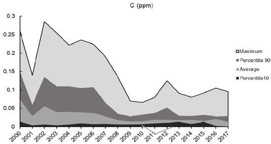
Figure 1.
Emissions of SO2 in Salamanca 2000–2017. Source: Adapted from INECC [18]. Note: Upper light gray indicates the maximum level of SO2 emission, dark gray shows the percentile 90th; the band gray below shows the average and finally the dark band indicates the 10th percentile of emissions registered by the red cross station during the signal period.
In this context, this study aimed to simulate SO2 dispersion from TPP chimneys to analyze the concentration profile from the emission point to the urban area, thus providing an approximation of the risk factors relating to health and the environment. The industrial chimneys of the Salamanca TPP are slender structures constructed with different materials, geometries, and dimensions for the evacuation of gases and fumes during the chemical process. This ensures the dispersion of SO2 effluents into the atmosphere to comply with the environmental regulations of the area where the source is located. NMX-AA-107-1988 established a minimum height for chimneys, which must not exceed the elevation of the formed turbulence zone of the surroundings due to the effects of wind on buildings or mountains and trees near the installation [18,19]. The same standard recommends that the inner diameter regulates the exit speed of gases to be between 15 and 25 m/s [20].
In the area of effluent pollutant dispersion, it is common to use the term plume or plumes to designate the column or cloud of effluent that exits a stack and is incorporated into the atmosphere [21]. Dispersion is the diffusion of atmospheric pollutants emitted by industrial processes. Its intensity is associated with various technical factors, such as the diameter and height of chimneys; speed and temperature of the gas effluent; meteorological factors, such as pressure, atmospheric temperature, wind speed, and direction [22]; and, finally, it is also a function of the topographic conditions (space) of the emission source and time [23], as shown in Table 2.
Table 2.
Geoenvironmental parameters.
The forms of pollution control suggested by the Environmental Protection Agency (EPA) include monitoring, which is diverse in terms of fixed or mobile technology [24], inventories, and modeling. Atmospheric dispersion models are an important tool for air quality management [25]. Simulation includes the latest knowledge on atmospheric dynamics to estimate the dissipation patterns, chemical reactions, and removal of such pollutants [26,27]. The numerical simulation of such phenomena models the dispersion and transport processes starting from data from the emitting sources. Other approaches employ advanced techniques, such as machine learning methodologies from different urban areas [28]. The mathematical description of pollutant transport in the atmosphere can be achieved using a parabolic-type second-order partial differential equation. In probability and statistics, the Gaussian distribution is used to analyze real events. In this particular case, the pollutant plume concentration depends on two longitudinal dimensions: the wind direction and the height of the plume. The mathematical model’s solution is a function of the technical parameters of the stack and atmospheric emissions, meteorological factors (wind speed, atmospheric temperature, and pressure), and ground roughness [29].
2. Gaussian Model Application (Simulation Method)
Simulation of 8 different SO2 dispersion sceneries of 4 chimneys was performed in the Salamanca TC. It was performed by applying a Gaussian model, by means of the function of the x-distance, measured from the stack base in the motion direction of the pollutant plume.
3. Study Area
Salamanca’s municipality and city are part of Guanajuato State’s most important industrial region, in the El Bajío industrial corridor. Economic relevance lies in the petrochemical industry, including a refining, chemical, automotive, and thermoelectric power plant. It has an area of 756.54 km2 and is located at 20° 34 13″ N latitude and 101° 11 50″ W longitude at an altitude of 1721 m above sea level. According to the Instituto Nacional de Estadística, Geografía e Informática, INEGI, it has 273,271 inhabitants [30]. The ONU HABITAT indicated that Salamanca’s municipality is in the basic index of prosperous cities but faces serious problems of atmospheric pollution due to emissions from the oil refining and electric power generation industries [31]. The Red Cross area also shows a high soil and water pollution ranking as one of the most polluted areas in Salamanca, Mexico (See Figure 2). Figure 3 shows the Red Cross Station location and the TPP. The tract and dispersion are indicated by the redline at which meteorological data and SO2 concentrations were obtained [32].
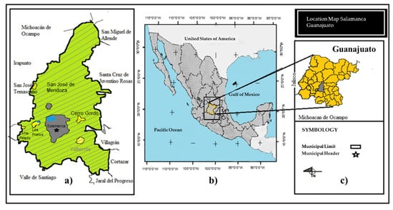
Figure 2.
(a) High soil and water pollution of the Salamanca entity, (b), Guanajuato location in the Mexican Republic Map (c) Salamanca, the most Polluted entity area in Guanajuato. Source: Adapted from Google Earth (2020) [32].
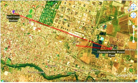
Figure 3.
Tract and dispersion of SO2 are indicated in the closest neighborhood on Salamanca’s Map from the TTP emission source monitored by the Red Cross station. Source: Adapted from Google Earth (2020) [32].
4. The Gaussian Model
Based on the assumption of the flux of matter per unit area and per unit time, Fick’s first law for molecular diffusion is used as follows:
where:
J = Mass flux of the pollutant (ML−2 T−1).
∂C = Concentration variation of the pollutant (ML−3).
∂x = Distance variation (L).
K = diffusion coefficient (L2 T−1).
The material balance assumes the following:
The solution of this one-dimensional equation is:
where Mo is the mass deposited at t = 0. The following formula is used:
where σx = turbulent dispersion coefficient (L).
It follows that:
In this one-dimensional equation, the concentration C is in units of mass per unit length (M/L).
For three-dimensional flow, the relationship must be extended by defining the turbulent dispersion coefficients σx, σy, and σz for the x, y, and z directions, respectively, such that:
Equation (6) solves the emission of a point source and allows the pollutant mass to be identified using Gaussian distribution equations. When it comes to an industrial chimney discharge, the phenomenon is studied in two dimensions. When dispersion is placed on the x axis, this can be ignored, since on this axis, only transport of pollutants due to the effects of wind occurs, although it would be interesting to study the dynamics of atmospheric turbulence in the y and z directions. For a 2-dimensional scattering processes involving the horizontal direction (y axis) and vertical direction (z axis), the equation is reduced to:
Along the horizontal axis (y axis), mass is assumed to be unproblematic for particle deposition, but on the vertical axis (z axis), it is deposited at a height H called the effective emission height; therefore, an axis shift must be performed using the following equation:
Furthermore:
The mass Mo can be determined by the relationship:
where:
Q = emission rate of the gaseous pollutant (MT−1).
U = average wind speed (LT−1).
After making the substitution, the above equation results in a mathematical expression of the two-dimensional Gaussian model:
The concentration at ground level is of significant interest in this study, so it is considered at y = 0 and z = 0. Therefore, Equation (11) is expressed as:
For the solution of Equation (12), some considerations were made:
Theoretical considerations.
- The stack is a point source of emission.
- The terrain where the dispersion of pollutants takes place is flat.
- The pollutant flow is incompressible.
- Turbulent flows are related to the gradients of the average concentrations.
- Pollutant diffusion is passive.
- Longitudinal diffusion and molecular diffusion are minimal and can be neglected.
- Both lateral and vertical wind speeds are considered to be zero.
- The location of the emission chimney, EC, stack is rural, according to its geographic coordinates and the shortest distance to the population.
- It is assumed that the transport of pollutants occurs in a straight line, instantaneously, in the wind direction.
Some considerations were also made to obtain the dispersion coefficients (σy and σz).
Table 3 shows that σy and σz are a function of the atmospheric stability category (ASC), and the distance on the x-axis, measured from the base of the stack in the direction of the plume [29].
Table 3.
Pasquill–Gifford dispersion coefficients of Briggs’s interpretation.
The Gaussian distribution indicates y = 0, where the pollutant is most concentrated is in the transverse y coordinate, since it coincides with the wind direction or studies related to the dispersion of stationary sources (see Figure 4).
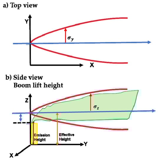
Figure 4.
Dispersion coefficients. (a) Top view of dispersion σy, (b) dispersion z exe, σz. Source: own elaboration and adapted from the two-dimensional Gaussian model [29].
There are two ways in which the dispersion coefficient can increase, which mathematically represents the width of the Gaussian bell, which means that the concentration of the pollutant decreases due to atmospheric dilution: when the x-distance, measured from the foot of the chimney increases, and when the atmospheric instability increases. This means that turbulence facilitates the dispersion of pollutants. So, at night and in rural areas, the dispersion coefficients are smaller [21].
Wind speed considerations:
For heights less than 10 m, wind speed is affected by friction and must be corrected by the following equation:
where:
Uz = wind speed at the height of the emitting source (m/s).
U10 = wind speed at the 10 m height (m/s).
h = height of the emitting source (m).
p = atmospheric exponential coefficient of the urban or rural environment according to the stability category (see Table 4).
Table 4.
Correction for wind speed.
Considerations for the effective height H:
To obtain the effective emission height (H), it is necessary to consider the plume height (Δh) plus the stack height (h) as indicated in the following equation:
The calculation of Δh requires other atmospheric parameters (temperature and pressure) and stack data, such as the diameter and pollutant exit velocity. Δh can be obtained using Holland’s equation [33]:
where:
Vs = pollutant exit velocity (m/s).
D = diameter of the chimney (m).
P = atmospheric pressure (mbar).
Ts = SO2 outlet temperature (°K).
Ta = atmospheric temperature (°K).
2.68 × 10−3 = constant (1/m mbar).
Plume height correction (Δh) is achieved using the Paquill–Gifford–Tunner factor shown in Table 5.
Table 5.
Factors of plume elevation.
5. The Origin of the Data
The statistical average was obtained from Red Cross station environmental data historical values of the variables, temperature, and atmospheric pressure at the Secretary of Environment and Territorial Planning of Guanajuato official site in 2017 [34]. Validation of the results was performed using the four thermal power plant stacks. The SO2 concentrations, technical data regarding the dimensions, and pollutant emissions were obtained from the same source [14].
6. Meteorological Data and SO2 Concentration Data
The historical Red Cross Station quality data were analyzed [34] to calculate the monthly and annual average pressure, temperature, wind speed, and direction. Figure 5a shows the monthly average 24 h pressure, which varies between 621.3 and 624.8 mmHg, while the temperature under the same conditions ranges from 17.8 to 22.5 °C in 2017. In Figure 5b, the monthly average SO2 concentrations range between 2.64 and 14.96 μg/m3. Meanwhile, the maximum and minimum values were recorded in the warm and cold seasons, respectively.
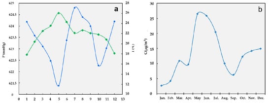
Figure 5.
(a) 24 h average atmospheric pressure and room temperature and (b) 24 h SO2 average concentration. Source: own elaboration.
The predominant wind direction through the WRPLOT View by Lakes Environmental Software (Waterloo, Ontario, Canada) is in a westerly direction, right at the Red Cross station (RCS). The monthly average wind speed varies between 0.45 and 8.34 m/s, according to the historical data reported by the official site, as shown in Figure 6.
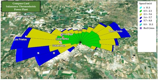
Figure 6.
Wind at the RC station Google Earth. Source: Adapted from Google Earth 2020.
Figure 7 shows the meteorological conditions (room temperature, barometric pressure, wind speed, time of day, and atmospheric stability conditions) that were considered in the modeling approach.
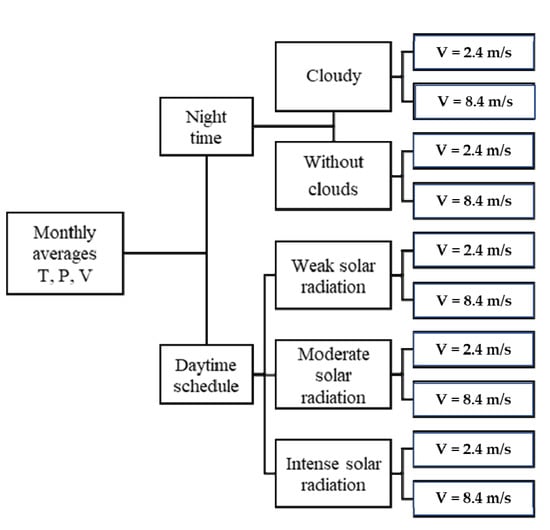
Figure 7.
Modeling sceneries.
The daytime and nighttime dispersion categories of Pasquill–Gifford–Turner were using to establish the modeling sceneries, as shown in Table 6. The SO2 concentrations and meteorological conditions, including room temperature and wind speed, were obtained from the data already mentioned in this section.
Table 6.
Pasquill–Gifford–Turner dispersion categories.
The Gaussian model assumes that meteorological conditions do not change over a considerable period of time. So, the model scenery approaches a set of conditions with an average minimum and maximum annual wind speed of 2.4 and 8.4 m/s, respectively, in Salamanca city.
Regarding temperature, the monthly average during the day and night was 24.2 and 19.2 °C, respectively. Moreover, three types of solar irradiation were contemplated: strong, moderate, and light. The Pasquill–Gifford–Turner ASCs were A, B, and C, respectively. During the night (cloudy and cloudless), the ASC scenarios were E and F. For a maximum average wind speed of 8.4 m/s, three types solar irradiation were considered based on the following Pasquill–Gifford–Turner ASCs: C and D. During the night (cloudy and cloudless), the only anticipated ASC scenario was D. Based on the total emissions obtained, the sum of the four stacks’ SO2 concentration was assumed to be representative of an annual cycle (see Table 7).
Table 7.
Scenarios and conditions of the modeling variables according to ASC.
Table 8 shows the modeling variables and technical SO2 emission and design data for the four stacks, which considered the information from the application of the model.
Table 8.
Stack data, emissions, and geographic and meteorological conditions.
7. Results
In agreement with the literature results [26,27,35], the importance of health risk management in highly industrialized cities is highlighted in in all models. The variation in the SO2 concentration from the base of the stacks up to 5000 m shows that at larger distances, SO2 pollution is reduced by dispersion. These results are demonstrated by the SO2 concentrations in the Gaussian model for the proposed scenarios.
The modeling of scenario 1 (Figure 8a) shows ASC A with strong and moderate irradiation at a wind speed of 2.4 m/s during the day in the 4 stacks: stack 1 recorded an SO2 concentration of 490 μg/m3 at 1000 m while stacks 2 and 3, with the same dimensions, reached a maximum value of 551 μg/m3 at 900 m. Finally, at 700 m, stack 4 reached a concentration of 355 μg/m3. With respect to the scenario modeling 2 with ASC B, the maximum SO2 concentrations (μg/m3) for stacks 2 and 3, 1, and 4 were 467 μg/m3 at 1500 m, 413 μg/m3 at 1500 m, and 301 μg/m3 at 1300 m (see Figure 8b), respectively. The results were above the limits established in the Official Mexican Standard, 2010 (NOM-DOF 2010).
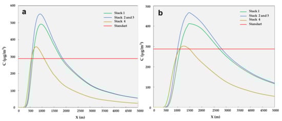
Figure 8.
(a) Scenario 1 and (b) scenario 2. Source: Author’s elaboration.
Figure 9a shows the results of the modeling scenario 3, ASC B, and the SO2 concentrations for stacks 2 and 3, 1, and 4 were 409 μg/m3 at 3000 m, 368 μg/m3 at 3000 m, and 280 μg/m3 at 2000 m, respectively, which are slightly below the maximum limits established in the Official Mexican Standard, 2010 (Official Mexican Norm Published officially in 2010) NOM-DOF 2010. For sceneries 4 and 5, ASC E and F, the SO2 concentrations, under partly cloudy and clear sky conditions and a relatively calm wind speed (2.4 m/s), were not detected in the Gaussian model due to an inherent flaw [29]. However, the detection of these concentrations using adequate models that precisely coincide with the worst conditions, which present greater risk, is relevant [22]. For scenario 6, ASC C, a wind speed of 8.4 m/s during the day was observed, and the maximum SO2 concentrations for stacks 2 and 3, 1, and 4 were 659 μg/m3 at 1000 m, 506 μg/m3 at 1100 m, and 380 μg/m3 at 900 m, respectively. These results are higher than the limits established in the Official Mexican Standard, NOM-022-SSA1-2010 (see Figure 9b).
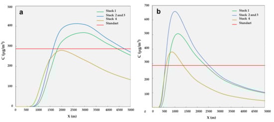
Figure 9.
(a) Scenery 3 and (b) scenery 4. Source: Author´s elaboration.
Figure 10a shows the results of scenario 7, ASC D, for a daytime wind speed of 8.4 m/s. The SO2 concentrations (μg/m3) for stacks 2 and 3, 1, and 4were 413 at 2000 m, 285 at 3000 m, and 242 at 1500 m, respectively. Finally, the modeling results of scenario 8, which corresponds to ASC D, at a velocity of 8.4 m/s during the night yielded the following SO2 concentrations (μg/m3) for stacks 2 and 3, 1, and 4: 412 at 2000 m, 285 at 3000 m, and 280 at 3000 m, respectively (see Figure 10b). Some authors in the literature have reported a decrease in the maximum concentrations of gaseous pollutants as the atmospheric instability decreases [29,36].
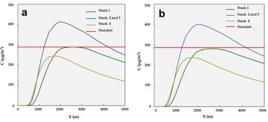
Figure 10.
(a) Scenary 7 and (b) scenery 8. Source: Author’s own elaboration.
Table 9 shows the profile of the maximum concentrations in the Gaussian modeling sceneries. The distances in the direction of the pollution plume at which the maximum SO2 concentrations were reached are reported.
Table 9.
Profile of the maximum SO2 concentrations at a distance (d) from the emission sources.
Regarding the wind trajectory, in all stacks, the emissions behavior exceeded the standard value (288 µg/m3) and was decreased by 12.15 %, 35.7 %, and 68.4 % at an average distance of 1,800 m, respectively. Larger distance values were found between 700 and 2000 m. Meanwhile, lower distance values were found at 3000 m. Finally, stacks 2 and 3 exceeded the emissions, reaching 485 µg/m3 at an average distance of 1933 m.
The vertical emission length did not represent a risk to the city due to the complete profile of the emission plume, which tended to descend as the horizontal distance increased. Overall, the Gaussian model showed that the average maximum SO2 concentration is 399 µg/m3, which is above the standard value (indicated by the maximum limits established in the NOM-022-SSA-010), at a distance of 1800 m. This considers the Red Cross (RC) monitoring station’s location at 3000 m. The best SO2 dispersion was obtained in scenario 8, corresponding to nighttime and at a relatively high speed 8.4 m/s and a concentration of 280 µg/m3, which are optimal values for a geographical site where, historically, wind conditions are calm. Concerning daytime, the best dispersion occurred in scenario 7 with high wind speed and strong solar irradiation. These results are similar to previously reported results [21,35]. Validation was performed based on the relative error in the SO2 emissions as shown by Equation 16:
where:
Er = relative error.
Cm = station concentration value (μg/m3).
Ce = estimated value (μg/m3).
The estimated value obtained for the stacks with the concentrations added at 3000 m was 1198 µg/m3, which was located at the RC station point. TPP emissions corresponded to 4.1% of the total SO2 emissions in the Salamanca municipality in 2017 [34]. Hence, the total emissions were 29,146 µg/m3. On the other hand, the measured value reported by the RC station was 34,191 µg/m3 and the absolute error was 14.7%. The model predicted more accurate values for the daytime dispersion phenomenon at moderate velocities between 2 to 3 m/s. This type of validation could be related to the pollutant stacks considered [37].
8. Discussion
Modeling is a valuable engineering tool for technology development for atmospheric monitoring, and its estimation. Its application to emission stacks allows for real-time air quality monitoring and control. Medium-term projections provide information for management evaluation strategies, which aim to comply with the national standards established by WHO. The maximum SO2 concentration profile results from the model revealed that during the day and night, the emission focus was the four chimneys of the Salamanca TPP where the concentrations reached residential areas. When the stability decreased in ASC A, B, and C, the maximum SO2 concentration also decreased.
The Gaussian model applied yielded an error close to 15%, representing a valuable mathematical tool for the generation of scientific evidence of the complex phenomenon of atmospheric pollutant dispersion to ground level. The model handles multiple variables (geographical, meteorological, such as temperature and atmospheric pressure, wind speed and direction) and design characteristics of the chimneys (height and diameter, and the type of fuels used on an industrial scale). Using this modeling process, some theoretical considerations, and others specific to the physical area where the study was carried out, allowed us to show the SO2 dispersion scenarios.
The findings show that, in a terrain of simple roughness, low wind speed, and ambient temperatures that are not extreme, as is the case of Salamanca city, SO2 dispersion in the horizontal path direction along the Gaussian plume exceeds the concentrations allowed during the day. A comparison with the calculation of the atmospheric dispersion coefficients employed in other mathematical formulations, such as Turner, Hosker, McMullen, or the Industrial Source Complex Short Term, ISCST models, CALPUFF model (California integrated Lagrangian PUFF modeling system), is suggested. It is important to broaden the spectrum to study three dimensions to completely analyze the atmospheric dispersion phenomenon. This information could be useful for the activation of transversal projects of a technical or epidemiological nature, using cleaner fuels, such as natural gas, to reduce SO2 and PM10 emissions (pollutants that trigger the activation of environmental pre-contingencies) from the effluents of TC chimneys, thus reducing health risks in the population.
9. Conclusions
The production of electricity from fuel oil showed severe implications on climate change and the health of inhabitants due to SO2 emissions, which require greater vigilance. The atmospheric monitoring station in Salamanca city, Red Cross (RC), found that meteorological conditions do not change over a considerable period of time and that the model scenery is related to gradients, such as the wind speed, dispersion, and the concentration of particulate material, such as SO2, which are related to the atmospheric stability category. The maximum average SO2 concentration was 399 µg/m3 at an average distance of 1800 m. In the scenarios comparison, scenery 8 showed better results. The nocturnal dispersion showed a maximum wind speed of 8.4 m/s and an SO2 concentration of 280 µg/m3 for stack 4, which is an atypical situation due to the geography of the city. From the validation process, a relative error of 14.7% was obtained, which indicates the reliability of the applied Gaussian model. Regarding the mathematical solution of the model, this represents a reliable and low-cost tool that can help improve air quality management, the location or relocation of atmospheric monitoring stations, and migration from the use of fossil fuels to environmentally friendly fuels.
Author Contributions
Data curation: A.E.V.G.; Formal analysis: R.d.J.P.C. and M.A.Y.C.; Funding acquisition: L.A.D.L.; Methodology: R.d.J.P.C. and M.A.Y.C.; Project administration: W.E.S.G. and J.d.C.Z.L.; Resources: J.d.C.Z.L. and L.A.D.L.; Software: R.d.J.P.C.; Supervision: W.E.S.G.; Validation: M.A.V.; Visualization: W.E.S.G., J.C.C. and E.G.V.; Writing – original draft: A.E.V.G.; Writing – review & editing: M.A.Y.C. All authors have read and agreed to the published version of the manuscript.
Funding
This research received no external funding.
Institutional Review Board Statement
Not applicable.
Informed Consent Statement
Not applicable.
Data Availability Statement
Not applicable.
Acknowledgments
The authors would like to thank the SMAOT of the government of the state of Guanajuato for their support in obtaining data for this study.
Conflicts of Interest
The authors declare not conflicts of interest.
References
- Etchie, T.O.; Etchie, A.T.; Adewuyi, G.O.; Pillarisetti, A.; Sivanesan, S.; Krishnamurthi, K.; Arora, N.K. The gains in life expectancy by ambient PM2.5 pollution reductions in localities in Nigeria. Environ. Pollut. 2018, 236, 146–157. [Google Scholar] [CrossRef] [PubMed]
- Molepo, K.M.; Abiodun, B.J.; Magoba, R.N. The transport of PM10 over Cape Town during high pollution episodes. Atmos. Environ. 2019, 213, 116–132. [Google Scholar] [CrossRef]
- Matus, P. Contaminación atmosférica: La composición química incide en su riesgo. Rev. Médica De Chile 2017, 145, 7–8. [Google Scholar] [CrossRef] [PubMed]
- Salini, G.A.; Medina, E.J. Estudio sobre la dinámica del material particulado PM10 emitido en Cochabamba, Bolivia. Rev. Interam. De Contam. Ambient. 2017, 33, 437–448. [Google Scholar] [CrossRef]
- Borrego, C.; Ginja, J.; Cuotinho, M.; Ribeiro, C.; Karatzas, K.; Simouis, T. Assessment of air quality microsensors versus reference methods: The EuNetAir Joint Exercise - Part II. Atmos. Environ. 2018, 193, 127–142. [Google Scholar] [CrossRef]
- WHO. Air Pollution. Obtenido de WHO Global Ambient Air Quality Database (Update 2018). Available online: https://www.who.int/airpollution/data/cities/en/ (accessed on 20 July 2019).
- CEMDA. Los Derechos Humanos y la Calidad de Aire en México; Hewlett Fundation: Ciudad de México, México, 2016. [Google Scholar]
- GREENPEACE. El aire que respiro. In El Estado de la Calidad del Aire; Obtenido de Greenpeace México A.C.: Ciudad de México, México, 2018; Available online: https://storage.googleapis.com/planet4-mexico-stateless/2018/11/ff412966-ff412966-aire_que_respiro_ok_emr.pdf (accessed on 11 November 2018).
- Ubilla, C.; Yohannssen, K. Contaminación atmosférica. Efectos en la salud respiratoria en el niño. Rev. Médica Condes 2017, 28, 111–118. [Google Scholar] [CrossRef]
- Pacsi, S. Análisis temporal y espacial de la calidad del aire determinado por material particulado PM10 y PM2,5 en Lima Metropolitana. Rev. An. Científicos 2016, 77, 273–283. [Google Scholar] [CrossRef]
- SEMARNAT. Comisión Federal Para la Protección Contra Riesgos Sanitarios. Obtenido de Clasificación de los Contaminantes del Aire Ambiente. Available online: https://www.gob.mx/cofepris/acciones-y-programas/2-clasificacion-de-los-contaminantes-del-aire-ambiente (accessed on 31 December 2017).
- SMAOT. Calidad del Aire. In Obtenido de Inventario 2017 de Emisiones de Contaminantes Criterio; Grandeza de Mexico: Guanajuato, Mexico, 2017; Available online: https://smaot.guanajuato.gob.mx/sitio/calidad-del-aire/4/Inventario-de-Emisiones-de-Contaminantes-Criterio (accessed on 16 October 2019).
- Instituto de Ecología del Estado. Informe de Estado y Tendencia; IEE: Guanajuato, México, 2016. [Google Scholar]
- CEPAL; ONU; SEMARNAT. Evaluación de las Externalidades Ambientales de la Generación Termoeléctrica en México; SEMARNAT: Ciudad de México, México, 2004. [Google Scholar]
- Instituto Para la Salud Geo Ambiental. El Dióxido de Azufre; 2020. Available online: https://www.saludgeoambiental.org/dioxido-azufre-so2?gclid=Cj0KCQiA8dH-BRD_ARIsAC24umaweBsq3109-VP_QODT9EtDklh9gYOPGgpeacfzs2N-PT8exkUjC8MaAjXIEALw_wcB (accessed on 5 January 2020).
- Ziberth, J.; Cedilnik, J.; Praznikar, J. Particulate matter (PM10) patterns in Europe: An exploratory data analysis using non-negative matrix factorization. Atmos. Environ. 2016, 132, 217–228. [Google Scholar] [CrossRef]
- Economic Commission for Latin America and the Caribbean (ECLAC). Economic Survey of Latin America and the Caribbean; (LC/G.2619-P); ECLAC United Nation Publication: Santiago, Chile, 2014. [Google Scholar]
- INECC. Informe Nacional de Calidad del Aire 2017, México. Coordinación General de Contaminación y Salud Ambiental, Dirección de Investigación de Calidad del Aire y Contaminantes Climáticos; INECC: Ciudad de México, México, 2018. [Google Scholar]
- Granados, A.S. Avances en el Análisis y Diseño de Chimeneas Industriales; UNAM: Ciudad de México, México, 2018. [Google Scholar]
- Legislación Ambiental. Norma Mexicana, Calidad del Aire. Estimación de la altura efectiva de chimenea y de la dispersión de contaminantes-método de prueba. Obtenido De Cent. De Calid. Ambient. 2020. Available online: http://legismex.mty.itesm.mx/normas/aa/aa107.pdf (accessed on 12 December 2020).
- Pereira-Peláez, D. Simulación de la dispersión de contaminantes en la atmósfera de una planta de generación de electricidad a biomasa. Acta Nova 2017, 8, 376–396. [Google Scholar]
- Trosic, T.; Filipcic, A. Multiple Linear Regression (MLR) model simulation of hourly PM10 concentrations during sea breeze events in the Split area. Naše More 2017, 64, 77–85. [Google Scholar] [CrossRef]
- Wang, C.Y.; Hsu, C. How critical is geometrical confinement? Analysis of spatially and temporally resolved particulate matter removal with an electrostatic precipitator. RSC Adv. 2018, 8, 30925–30931. [Google Scholar] [CrossRef]
- McKercher, G.R.; Salmond, J.A.; Vanos, J.K. Characteristics and applications of small, portable gaseous air pollution monitors. Environ. Pollut. 2017, 223, 102–110. [Google Scholar] [CrossRef] [PubMed]
- Gibson, M.; Kundu, S.; Satish, M. Dispersion model evaluation of PM2.5, NOX, and SO2 from point and. Atmos. Pollut. Res. 2013, 4, 157–167. [Google Scholar] [CrossRef]
- Amable, I.; Méndez, J.; Bello, B.; Benítez, B.; Escobar, L.; Zamora, R. Influencia de los contaminantes atmosféricos sobre la salud. Rev. Médica Electrónica 2017, 39, 2470–3610. [Google Scholar]
- Kelly, J.T.; Jang, C.J.; Timin, B.; Gantt, B.; Reff, A.; Zhu, Y.; Long, S.; Hanna, A. A system for developing and projecting PM2.5 spatial fields to correspond to just meeting national ambient air quality standards. Atmos. Environ. X2 2019, 2, 100019. [Google Scholar] [CrossRef] [PubMed]
- Alimissis, A.; Philippopoulos, K.; Tzanis, C.G.; Deligiorgi, D. Spatial estimation of urban air pollution with the use of artificial neural network models. Atmos. Environ. 2018, 191, 205–213. [Google Scholar] [CrossRef]
- Cruz-López, C.A. Implementación de un Modelo de Dispersión Atmosférica y Cálculo de Dosis en la Liberación de Efluentes Radiactivos en el Centro Nuclear. Tesis; IPN: Ciudad de México, México, 2015. [Google Scholar]
- INEGI. INEGI. 2017. Available online: http://www.inegi.org.mx/ (accessed on 12 December 2020).
- ONU HABITAT. Available online: http://infonavit.janium.com/janium/Documentos/57878.pdf (accessed on 11 August 2016).
- Google Earth. Localización de Salamanca, Gto. 2020. Available online: https://earth.google.com/web/@20.56991452,101.17962351,1711.86259827a,3811.42382427d,35y,0h,0t,0r.34 (accessed on 12 December 2020).
- Molano, L.G.; Díaz, C.J. Análisis y verificación del modelo gaussiano de dispersión: Métodos teóricos y experimentales. Rev. De Investig. 2019, 12, 31–43. [Google Scholar] [CrossRef]
- SMAOT. Datos Históricos de la Calidad del Aire. 2020. Available online: https://smaot.guanajuato.gob.mx/sitio/seica/historicos/salamanca (accessed on 12 December 2020).
- Li, P.; Peng, L.; Yao, X.; Cui, S.; Hu, Y.; Yuo, C.; Chi, T. Long short-term memory neural network for air pollutant concentration predictions: Method development and evaluation. Environ. Pollut. 2017, 231, 997–1004. [Google Scholar] [CrossRef] [PubMed]
- Zambrano, M.E. Análisis de Dispersión de Contaminantes Emitidos por Motores Que Utilizan Petróleo Crudo Como Combustible; Health Universitat de Barcelona: Informe Barcelona, España, 2017. [Google Scholar]
- Madrazo, J.; Clappier, A.; Belalcazar, L.C.; Cuesta, O.; Contreras, H.; Golay, F. Screening differences between a local inventory and the Emissions Database for Global Atmospheric Research (EDGAR). Sci. Total Environ. 2018, 631–632, 934–941. [Google Scholar] [CrossRef] [PubMed]


Publisher’s Note: MDPI stays neutral with regard to jurisdictional claims in published maps and institutional affiliations. |
© 2022 by the authors. Licensee MDPI, Basel, Switzerland. This article is an open access article distributed under the terms and conditions of the Creative Commons Attribution (CC BY) license (https://creativecommons.org/licenses/by/4.0/).