A New Look into the South America Precipitation Regimes: Observation and Forecast

Abstract

South America is a vast continent characterized by diverse atmospheric phenomena and climate regimes. In this context, seasonal climate predictions are helpful for decision-making in several relevant socioeconomic segments in this territory, such as agriculture and energy generation. Thus, the present work evaluates the performance of ECMWF-SEAS5 in simulating the South American precipitation regimes by applying a non-hierarchical clustering technique. In addition, the study describes the main atmospheric systems that cause precipitation in each cluster and updates a previous work performed in South America in 2010. As a result, ECMWF-SEAS5 simulates (with good correspondence) the eight climate regimes identified in the analysis of precipitation from the Climate Prediction Center (CPC). Moreover, ECMWF-SEAS5 has a satisfactory ability in representing the rainfall regime in low and medium climate predictability regions, such as central and southern South America. ECMWF-SEAS5 has good performance in the climate characterization of South America and it gives us confidence in using its seasonal climate predictions throughout the continent.

1. Introduction

South America (SA) is a continent with a wide meridional extension (12° N–55° S) and complex topography [1]. Moreover, SA owns heterogeneous geography, enfolding the existence of particular features (e.g., the Andes Cordillera and the Amazon Forest) and dry regions (e.g., the Atacama Desert and the semiarid Northeast of Brazil) (Figure 1). Such aspects favor the occurrences of different atmospheric systems and climate contrasts in its vast territory, as described by Reboita et al. [1].

The Andes has the longest cordillera in the world, and it extends across the western SA from Patagonia to Venezuela, encompassing a variety of climate features, such as humid conditions in the tropics and western Patagonia in the extratropics, and dry conditions in the subtropics, as in the Atacama Desert [2,3]. Moreover, the Andes concentrate more than 99% of all tropical glaciers [4], of which 71% are in Peru and 20% in Bolivia [5], supplying biodiversity and ecosystem services, such as fresh water to about 90 million people in seven countries (Venezuela, Colombia, Ecuador, Peru, Bolivia, Chile, and Argentina) [3,6]. Likewise, Andean countries, such as Bolivia and Peru, have considerable dependence on the glacier mountains for the feasibility of various socioeconomic activities, including the supply of water to hydropower plant reservoirs and the development of tourism [7,8,9,10,11]. However, the Andes are particularly vulnerable to climate change effects, urbanization, deforestation, and land-use changes [7,8,9,10,11,12,13,14].

The Amazon rainforest is another crucial sector of South America. The Amazon biome is the largest tropical rainforest in the world and comprises more than 35% of SA territory [15], besides providing about 20% of all the world’s fresh water [16] and playing an essential role in global energy, moisture, and carbon balances [17,18]. The Amazonian region also hosts the greatest biodiversity globally [19] and has an enormous cultural and ethnic richness composed of around 450 Indigenous groups and more than 250 languages [20]. Despite its paramount importance, the biome is susceptible to climate change and other threats, such as fires, grazing intensification, and deforestation [21]. After a decline during the early 21st century [22], deforestation and fires have increased, reaching almost a fifth of the territory [18,23]. Consequently, the Amazon rainforest is prone to a biophysical tipping point, a threshold exceeded due to anthropogenic pressures, such as fires and deforestation, and indirect pressures through climate variability, which can transform a tropical and biodiverse ecosystem into a drier or savannized environment [21,22,23,24,25,26,27].

SA presents prominent meridional and zonal variations in climate regimes [15]. The northern and central parts of SA have tropical patterns, the western portion of the continent owns arid and steppe climates, the southeast is considerably temperate, and the southwestern edge has a polar tundra climate [28]. SA also shows expressive climate contrasts, exemplified by the existence of both one of the wettest areas (Colombian region) [29] and driest regions on the planet, such as the Atacama Desert in western Chile [30,31] and the semiarid northeast of Brazil [32,33,34].

SA also has remarkable seasonal variability in precipitation, with a large band from south Amazon to southeast Brazil experiencing a wet, warm summer (DJF) and a dry, mild period in the winter (JJA) [35,36,37,38,39,40,41,42,43,44,45,46,47,48,49,50,51,52]. Because most of the precipitation is concentrated in DJF, the climate of this area is classified as a monsoon. It is worth mentioning that through the classical definition of a monsoon pattern, based on seasonal wind reversal [53], SA would not be considered a monsoon region since this continent does not show seasonal reversal of winds between January and July [54]. However, through the modern definitions that consider the difference in precipitation between winter and summer, SA is classified as a monsoon climate region, and the combination of atmospheric systems responsible for the precipitation is called the South American Monsoon System (SAMS) [1,35,36,37,38,39,40,41,42,43,44,45,46,47,48,49,50,51,52,54]. SAMS has two well-defined seasons: the rainy season from November to March and the dry season from May to September. Different circulation systems at upper and lower levels of the atmosphere characterize these two periods [1,35,36,37,38,39,40,41,42,43,44,45,46,47,48,49,50,51,52,54].

The wet phase of SAMS begins to emerge from the austral spring when there is an intensification of solar energy received in the Southern Hemisphere and, as a consequence, convection becomes stronger. Additionally, the trade winds intensify and transport more moisture from the tropical North Atlantic to the Amazon Basin [45,55,56]. Due to the surface heating and convective activity, an area of high pressure is formed at high levels over the continent, known as the Bolivian High (BH) [57,58]. Downstream of the BH, a trough develops between northeast Brazil and the Atlantic Ocean, called the Northeast Trough (NT) [57,58]. In the wet phase of SAMS, at the low troposphere, two low-pressure centers are formed east of the Andes Mountains, the Chaco low (CL) and the northwestern Argentinean low (NAL), influencing weather conditions mainly in north-central Argentina, southern Bolivia, and Paraguay [59,60]. Similarly, these lows are crucial for the South American low-level jet (SALLJ) east of the Andes configuration, as they produce a horizontal pressure gradient with the Amazon region [60]. SALLJ is responsible for transporting moisture from the Amazon Basin to the southeastern region of SA, which includes northern Argentina, Paraguay, Uruguay, and southern/southeastern Brazil [61,62].

The coupling of the summer local convection with the warm and moist air from the tropics to the subtropics by the SALLJ and by the northeast winds of the South Atlantic subtropical anticyclone (SASA) [63] originates the South Atlantic convergence zone (SACZ) [38,64,65,66] (Figure 2a). SACZ corresponds to a band of clouds extending from the Amazon to southeastern Brazil and reaches the South Atlantic Ocean, configuring one of the most relevant systems for maintaining rainfall over SA during the monsoon’s wet phase. In periods without or with weak SACZ activity, SALLJ generally transports moisture to the southeast of SA or northern Argentina (Figure 2b), influencing precipitation in the La Plata Basin (LPB) [45,67]. On the other hand, when the SALLJ is directed towards southeastern Brazil, it activates the SACZ [65]. Figure 2 illustrates a schematic representation of these systems in SA, considering two scenarios: when SACZ occurs and without SACZ.

The realistic representation of South American climate features remains a challenge for numerical models [15,68,69,70,71,72,73,74,75]. Global climate models (GCMs) reproduce and predict the main characteristics of precipitation, temperature, and circulation over the continent. Nevertheless, they fail in simulating regional climate over terrains with a complex topography and still show systematic rainfall biases in regions such as tropical SA, Andes, and La Plata Basin (LPB) [15,68,69,70,71,72,73,74,75]. In the SACZ region, limitations persist since summer rain predictability over the SACZ area is lower over the continent than in the ocean [76,77]. Furthermore, GCMs are unsuitable for reproducing the ocean–atmosphere coupling associated with SACZ and the Intertropical Convergence Zone (ITCZ) activity [77].

Since SA has many peculiarities in its climate, Reboita et al. [1] summarized the SA rainfall regimes based on the annual cycle of precipitation pattern, distributing the continent into eight regions with symmetric seasonality. However, these authors employed qualitative and visual evaluations of the SA climate based on precipitation data from 1931 to 1960 without an objective assessment method. So, there is still a gap in the literature for redoing this work with statistical methods, such as cluster analysis. Until now, studies involving a precipitation clustering process focused only on specific regions of the continent, such as the tropical SA [78], Bolivia [79], Argentina [80,81,82,83], Chile [84], Colombia [85], Ecuador [86], Brazil [87,88], and Brazilian sectors, such as the northeast [89,90,91,92,93,94], south and southeast [95,96,97], central-west [98], and the Amazonian portion [99].

In this scenario, the present study’s relevance is justified not only for identifying homogeneous rainfall regions in SA considering a recent period (1993–2016) and an objective methodology but also by evaluating the skill of last generation climate predictions provided by ECMWF for South American continent.

Given the background, the goals of this work were: (a) to apply a clustering technique to monthly rainfall data from the Climate Prediction Center (CPC) and European Centre for Medium-Range Weather Forecasts—System 5 (ECMWF-SEAS5) for the South American continent; (b) to validate the ECMWF-SEAS5 predictions through the assessment of its capability in simulating distinct rainfall patterns of SA and; (c) to describe the different groups obtained according to the main atmospheric systems that cause precipitation. The study’s novelty is that it applies an objective analysis, using two recent datasets provided by rainfall analyses (CPC) and state-of-the-art seasonal climate predictions (ECMWF-SEAS5), to describe the precipitation regimes over the whole continent and discuss the performance of ECMWF-SEAS5.

2. Materials and Methods

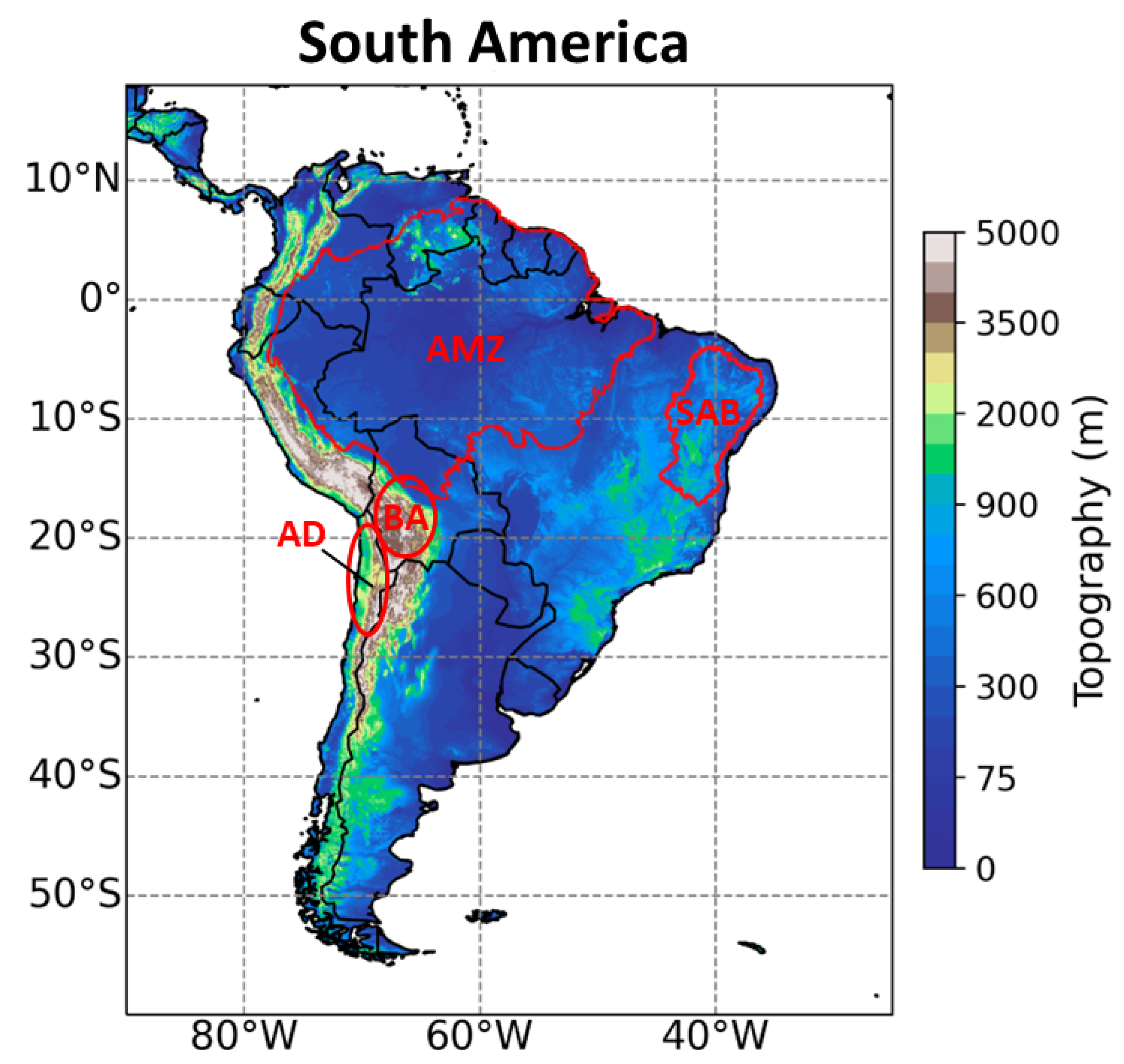
2.1. Study Area

The study area is illustrated in Figure 1 and comprises the South American continent. SA has a large meridional extension, located in tropical, subtropical, and extratropical latitudes, which gives the continent a complex climate diversity. In the same way, its heterogeneity of topography and vegetation reinforces the existence of different precipitation regimes in the SA territory.

2.2. Data

2.2.1. ECMWF-SEAS5

ECMWF-SEAS5 is the latest generation of seasonal climate predictions from the European Centre for Medium-Range Weather Forecasts and has been in operation since 2017. The present study used seasonal precipitation predictions (total accumulated rainfall every 24 h since the start of the forecast) provided by hindcasts from 1993 to 2016.

Following the operational seasonal forecasting methodology, the hindcasts (the system’s climatological model constituted by predictions of past conditions) were initialized on the first day of each month and were composed of a 25-member ensemble (whilst the operational forecast ensemble owns 51 members). The ensemble was created using perturbations to the atmospheric and oceanic initial conditions, sea surface temperature (SST), and activation of stochastic physics [100]. The ensemble technique is essential because it quantifies the effects of errors due to the model’s limitation and uncertainties in the initial conditions and provides information about the forecasts’ reliability [100]. Here, the arithmetic means of all ensemble members were used to compute monthly rainfall predicted by ECMWF-SEAS5.

Forecasts were integrated for seven months, but only the second month of prediction (a 1-month lead time) was used in this work. For instance, for a forecast initiated on January 1, only the prediction of February mean rainfall is used. The first month of prediction is discarded due to the spin-up time, which is the time required for a coupled model to reach an equilibrium state under the applied forcing [101].

Seasonal climate predictions from ECMWF-SEAS5 are available with a horizontal resolution of 1° (accessible at https://cds.climate.copernicus.eu/cdsapp#!/dataset/seasonal-original-single-levels?tab=form, accessed on 13 May 2020). However, despite the resolution of data publicly available, the system’s dynamical processes (including the physical parameterizations) were solved on a grid of approximately 36 km² [100].

2.2.2. CPC and ERA5 Data

The Climate Prediction Center Gauge-Based Analysis of Global Daily Precipitation (CPC-Global) [102] generated by the National Oceanic and Atmospheric Administration/Climate Prediction Center (NOAA/CPC) was used to validate the ECMWF-SEAS5 predictions. CPC-Global is derived from thousands of rain gauges across the globe, cooperative observation networks, and meteorological agencies [103]. Data quality control is carried out through comparisons with historical records, surface measurements, radar and satellite observations, and predictions from numerical models [102]. Daily CPC data from 1993 to 2016 (available at https://ftp.cpc.ncep.noaa.gov/precip/CPC_UNI_PRCP/GAUGE_GLB/RT/, accessed on 12 August 2020) were used in this work. Since the CPC analysis has a horizontal resolution of 0.5°, data were interpolated to the spatial resolution of ECMWF-SEAS5 by the bilinear method [104].

ERA5 [105] data were used to represent the seasonal atmospheric circulations at lower and upper levels. These data include monthly zonal and meridional wind data at 200 hPa and 850 hPa for 1993–2016.

2.3. Cluster Analysis

The goal of cluster analysis is to statistically classify the elements of a sample (into groups) so that the elements belonging to the same group are similar to each other concerning the measured variables.

Clustering analysis methods can be hierarchical and non-hierarchical. A disadvantage of hierarchical methods is that they do not allow the relocation of points that have been misclassified in some previous stage. Clustering methods that enable the relocation of elements as the analysis proceeds are called non-hierarchical. Non-hierarchical methods start the process from an initial partition of items in groups or a set of initial centroids. Both methods group data according to a distance measure in the k-dimensional element space [106].

In the hierarchical method, small biases in the variables may propagate, inducing larger deviations in the subsequent steps since the relocation of the clustered data is not allowed. In contrast, the non-hierarchical method, being a continuously divisible process, is less likely to be affected by noises in the data [107]. On the other hand, a disadvantage of non-hierarchical clustering is the need to choose the number of clusters a priori [108]. In any manner, despite the diversity of approaches, there is no clustering technique universally judged to be the best, and different algorithms can provide different groupings [89].

In general, cluster analysis studies of precipitation in SA regions use hierarchical methods [78,80,81,82,85,87,89,90,91,92,93,94,95,96,97,98,99], given that these techniques provide satisfactory results and have a variety of clustering methods and several dissimilarity metrics to categorize the variables into homogeneous groups [91]. Considering the non-hierarchical method, the few existing studies in SA examine specific regions of the continent, such as Bolivia [79], Argentina [83], Chile [84], and Ecuador [86]. Whilst there is a scarcity of works using the non-hierarchical clustering for the whole SA, studies that employed the method in Africa [107] and Europe [108] concluded that the methodology guarantees good results and is appropriate for analyzing precipitation regimes.

One of the most popular ways of non-hierarchical clustering is the K-means method. Examining hierarchical and non-hierarchical clustering methods, Zhang et al. [107] concluded that the K-means method results better than hierarchical techniques (low WSS, high intra-correlations, and low intercorrelations) and is more suitable for cluster analyses of complex climate datasets.

The K-means method computes the centroids for each cluster and then calculates the distances between the data vector and each centroid, grouping the vector to the cluster whose centroid is closest to it. This process is repeated until all vectors are grouped into a cluster whose members are closer to the centroid than the other clusters’ average [106].

From the definition of the initial k number of clusters, the K-means method proceeds according to the following steps:

(1)

Compute the centroids for each cluster;

(2)

Group the elements according to the most similar centroid;

(3)

Recalculate the centroid for each cluster that receives the new element and for the cluster that loses the element;

(4)

Repeat steps 2 and 3 until all elements converge.

This procedure produces k clusters with the k cluster mean or centroids, and the within-cluster sum of square errors (WSS) will be minimized according to Equation (1):

$$\mathrm{the} \mathrm{WSS}={\displaystyle \sum }_{\mathrm{j}}^{\mathrm{k}}{\displaystyle \sum }_{\mathrm{g} \in \mathrm{j}}{\left({\mathrm{t}}_{\mathrm{g}}-{\overline{\mathrm{t}}}_{\mathrm{j}}\right)}^2$$

(1)

where $\mathrm{WSS}$ is the sum of the squared errors between the time series at each grid point $\mathrm{g}$ (${\mathrm{t}}_{\mathrm{g}})$ in cluster $\mathrm{j}$ ($\mathrm{g}\in \mathrm{j})$ and the average time series in cluster $\mathrm{j}$ (${\overline{\mathrm{t}}}_{\mathrm{j}}$, known as the mean or centroid) and then summed for all $\mathrm{k}$ clusters [106,107]. WSS measures the variability of elements within each cluster, which means that a cluster with a low WSS is more compact than a cluster with a large WSS.

Despite the non-hierarchical method objectiveness, the choice of k is still a subjective task. One way to evaluate the number of clusters is through the Elbow method, which evaluates the performance of WSS related to the increasing k number of clusters [107,109]. However, the Elbow method can be problematic in fields such as hydroclimatology, where many point grids are considered, but a relatively small number of clusters is desired [107]. Using the Elbow method and a verification suggested by Zhang et al. [107], we obtain k = 8 clusters, the same number defined empirically by Reboita et al. [1].

In this way, the K-means cluster execution involves the following steps:

(1)

Calculations of precipitation monthly means between January and December (1993–2016) derived from daily CPC data and predictions of daily accumulated rainfall for the 1-month lead time of ECMWF-SEAS5 seasonal climate forecasts;

(2)

Organization of the data giving a matrix of 1581 grid points per 12 months;

(3)

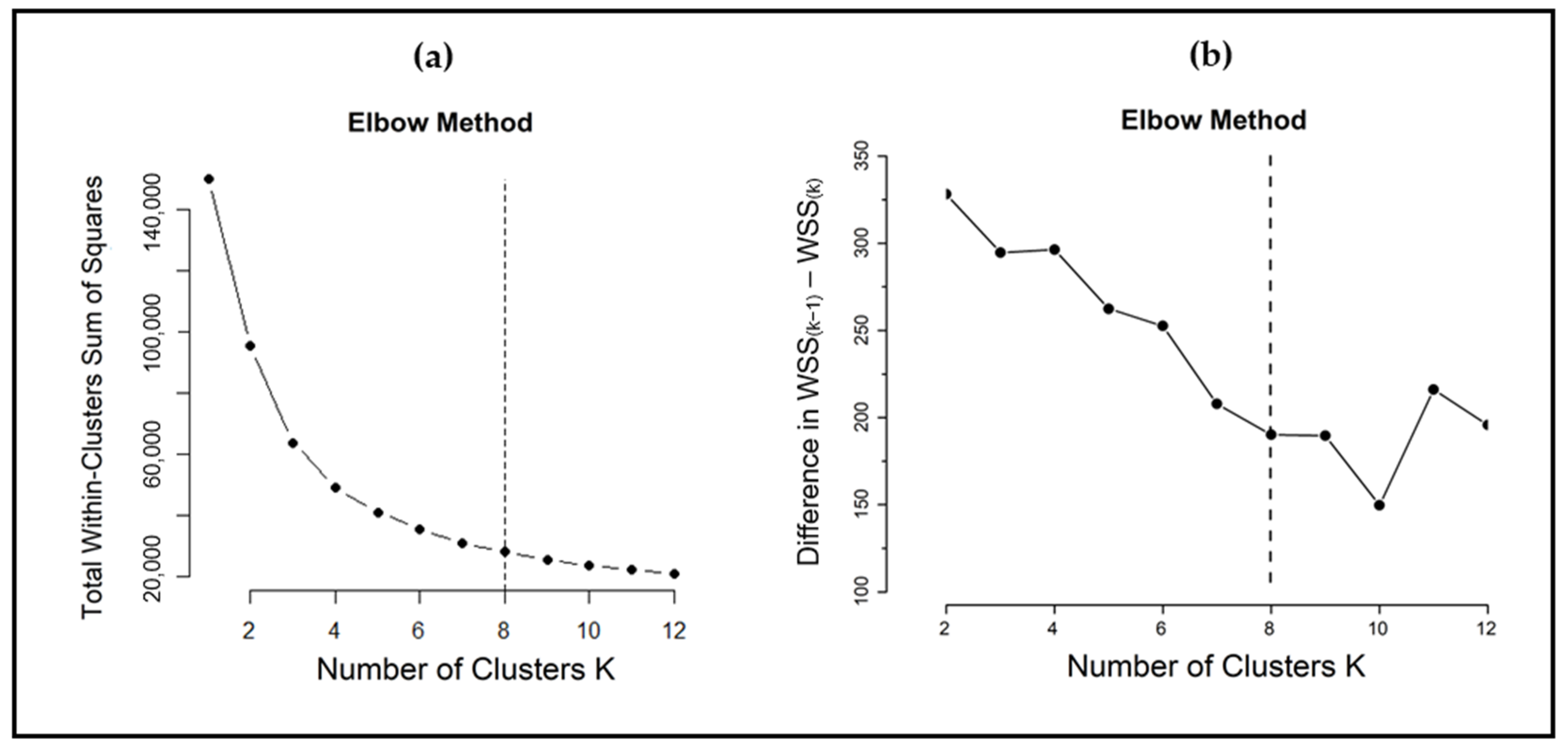
Application of the Elbow method and its derivation proposed by Zhang et al. [107];

(4)

Execution of the K-means algorithm through the Scikit-Learn library from the Python language [110].

After performing the preceding steps, it was possible to evaluate the clusters’ spatial distribution from both datasets and the correspondence of the obtained groups to the regions previously identified [1].

3. Results and Discussion

3.1. Elbow Method

The Elbow method evaluates how WSS behaves according to the increase in the number k of clusters to examine the percentage of variance explained as a function of the number of clusters. The number k of clusters is plotted linearly to identify when changes in WSS values are no longer expressive. At a given point, the marginal gain decays substantially and forms an angle in the graph. The optimal k number of clusters is chosen at this point, distinguished by forming an “elbow” in the plotted curve. Zhang et al. [107] state that the Elbow method is not the most suitable for this case since there is no well-established elbow due to a large number of point grids and the small number of desired clusters. This characteristic is evident in Figure 3a, which shows the curve obtained by the Elbow method derived from the K-means cluster analysis applied to CPC data for the entire SA region.

It was observed that the plotting of total WSS according to different k numbers of clusters does not evidence an optimal point for the selection of the groups’ quantity. Similar behavior was also obtained by Zhang et al. [107] when searching for the best number of clusters for the regionalization of seasonal precipitation in western Ethiopia. Furthermore, it was noticed that the curve presents a major inflection at k = 3, which may be due to a more compact classification of the algorithm when distributing precipitation in SA into tropical, subtropical, and extratropical domains. However, k = 3 is not a value of interest for application in the present study, given that it generalizes precipitation regimes into notoriously geographical groups and disregards the particularities of different precipitation patterns in SA.

An alternative way to evaluate the performance of WSS is calculated through the differences in WSS_k−1 e WSS_k [107]. Figure 3b illustrates the results provided by this method and indicates apparent points of change in the curve’s slope as the descending elbows at k = 3, k = 5, k = 7, k = 8 and k = 10, and the ascending ones at k = 4, k = 6, k = 9 and k = 11. Unlike the typical Elbow method, such an approach scrutinizes the decreasing rates of difference in WSS_(k−1)−k to locate the optimal k number, so that abrupt changes in the WSS_(k−1)−k curve can be captured [107].

Figure 3b indicates that the differences between WSS_k−1 and WSS_k for each k are relevant, pointing to considerable decay of WSS_(k−1)−k between k = 7 and k = 9. Since the other “elbows” (k = 3, k = 5, and k = 7) are not convenient numbers for the clustering objectives of the present study, k = 8 is considered a reasonable value to represent the main SA seasonal precipitation patterns. Moreover, it is supported by the previous work of Reboita et al. [1].

Figure 3 presents the Elbow method evaluation applied to the CPC data, but the same analysis was performed with ECMWF-SEAS5, which provided similar results. However, for brevity and because CPC represents the ground observed data in this work, only its results are presented.

Thus, given the K-means clustering performed with k = 8, the seasonal precipitation patterns were analyzed according to the different spatial clusters obtained. The following section discusses the main atmospheric systems that modulate the seasonal rainfall variability of South American regions resulting from the clustering analysis.

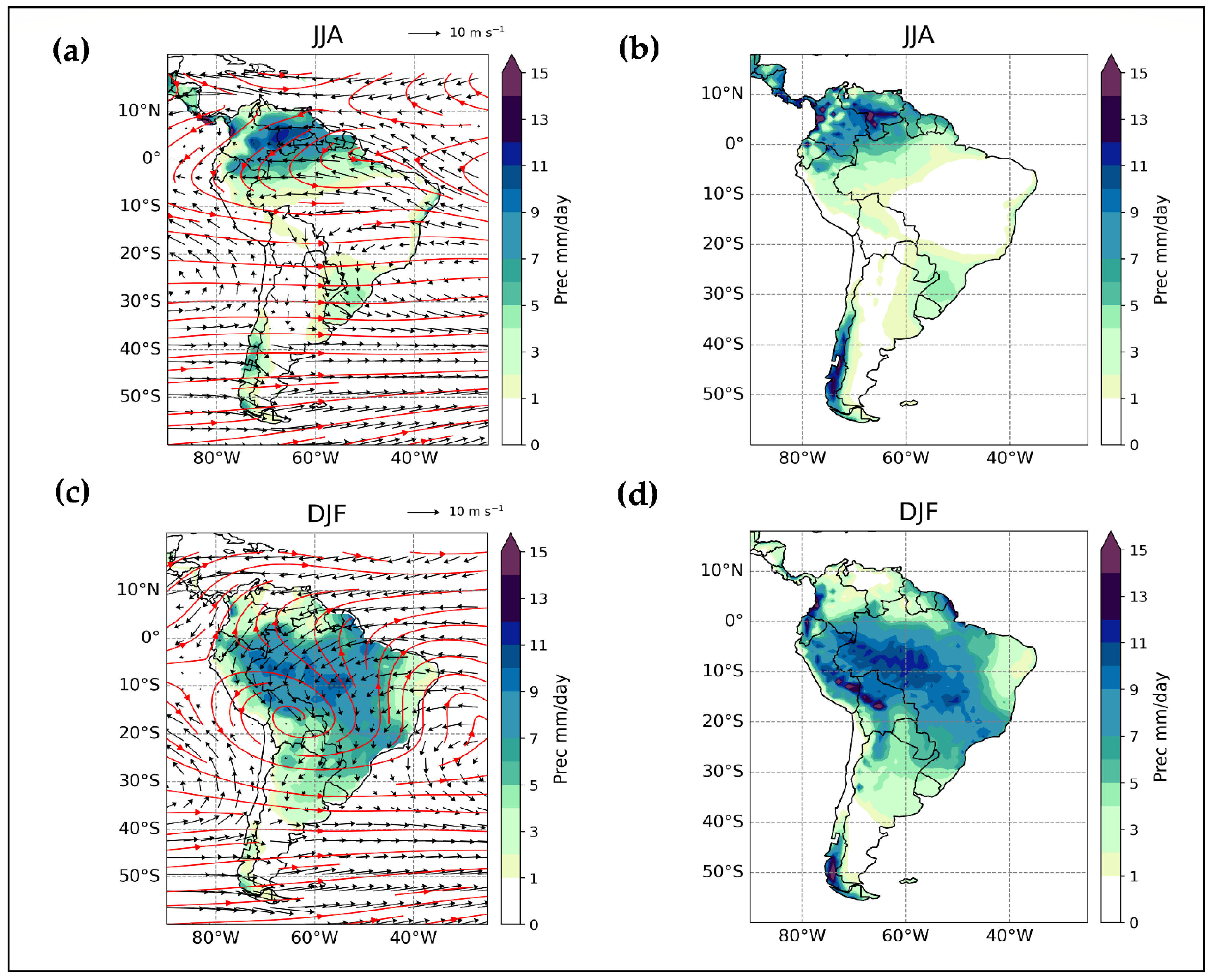
3.2. Climatological Features

Before the clustering results analysis, a brief presentation of the seasonal rainfall patterns and atmospheric circulation in SA is given. Then, it is possible to demonstrate some of the aforementioned atmospheric systems and evaluate the climatological precipitation simulation in the South American continent by ECWMF-SEAS5.

Figure 4a,b illustrate the mean climate patterns in SA during winter, characterized by maximum rainfall in the equatorial region of the continent (including northern Brazil and northern SA countries) and less precipitation over most of central and northeast Brazil, Argentina, Bolivia, and portions of Paraguay and Peru.

By comparing the rainfall outputs from the CPC with the ECMWF-SEAS5 hindcasts, it is observed that both have similar features, indicating a wetter pattern in northern SA and drier ones in the central and southern parts of the continent. However, despite correspondence between the results, it is noted that ECMWF-SEAS5 overestimates the rainfall volumes in the extreme south of SA (southwestern Argentina and southern Chile) and underestimates the variable in northeastern Brazil. During winter, SASA is located in its westernmost position, influencing the atmospheric circulation in the southeast and south of Brazil and sectors of Argentina, Bolivia, Paraguay, and Uruguay (Figure 4a). At upper levels, westerlies are zonally configured (Figure 4a).

Figure 4c,d present the mean climate patterns in SA during summer, indicating increased rainfall totals in central SA, including most of Brazil, northern Bolivia, and eastern Peru. The well-configured representation of the SACZ is evident, characterized by a band of greater precipitation that extends from the south of the Amazon region to the Atlantic Ocean, passing through the central–west and southeast of Brazil. Moreover, it is noted that portions of SA, such as southern Brazil and Uruguay, have less spatial and seasonal rainfall variability, as rainfall totals do not indicate substantial changes in the winter and summer seasons. Regarding the atmospheric circulation, Figure 4c shows the SALLJ acting and the eastward displacement of SASA, which contribute to the transport and higher moisture concentration in the SACZ region. There is a high-pressure region over Bolivia (Bolivian High) at upper levels, and downstream a trough is formed over northeastern Brazil (Northeast Trough). Figure 4c shows the seasonal climatology, including SACZ and non-SACZ days. The climatology only for SACZ is slightly different in atmospheric circulation, as shown in Figure 2a.

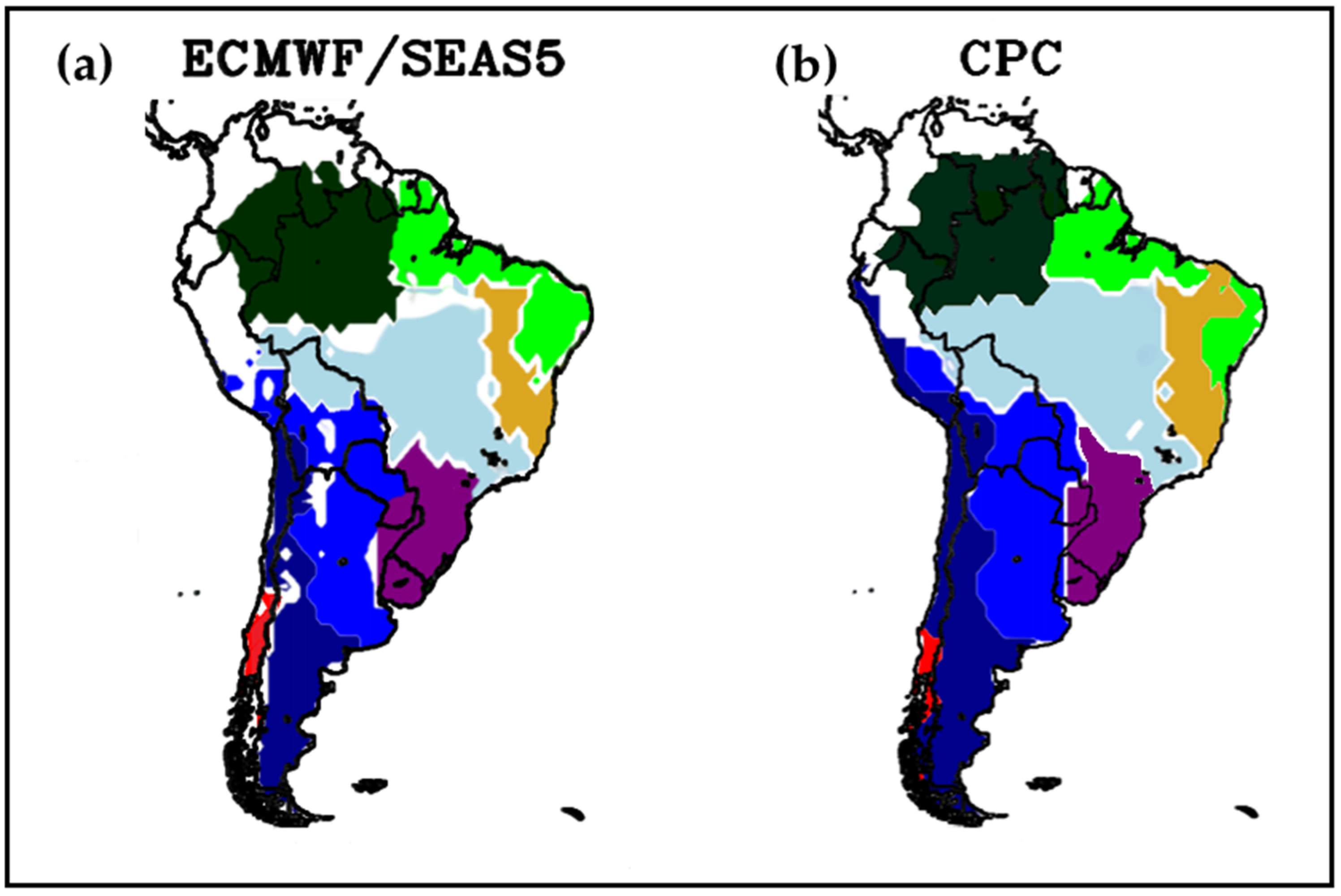
3.3. Regional Precipitation Clusters in South America

Figure 5 illustrates the eight clusters provided by the K-means method applied to the ECMWF-SEAS5 and CPC precipitation data for the South American continent. The clusters show spatial correspondence, with slight distinctions in regions such as northern Argentina and north-central Brazil, where ECMWF-SEAS5 indicates a little fragmented distribution. In addition, some sectors, such as northern Peru and northern SA, present considerable variability in the rainfall regime and miscellany of groups. As the purpose of this study was a synoptic scale view of the precipitation, we preferred not to show the cluster diversity to avoid a discussion about local climate features. Nevertheless, ECMWF-SEAS5 indicates a fair representation of the different groups that compose precipitation regimes in SA. Moreover, the homogeneous regions of rainfall identified in the present study corroborate the sectors found by the subjective approach of Reboita et al. [1] and the hierarchical clustering of Gubler et al. [111]. The following subsections describe the annual cycle of precipitation and the dominant atmospheric systems acting in each cluster.

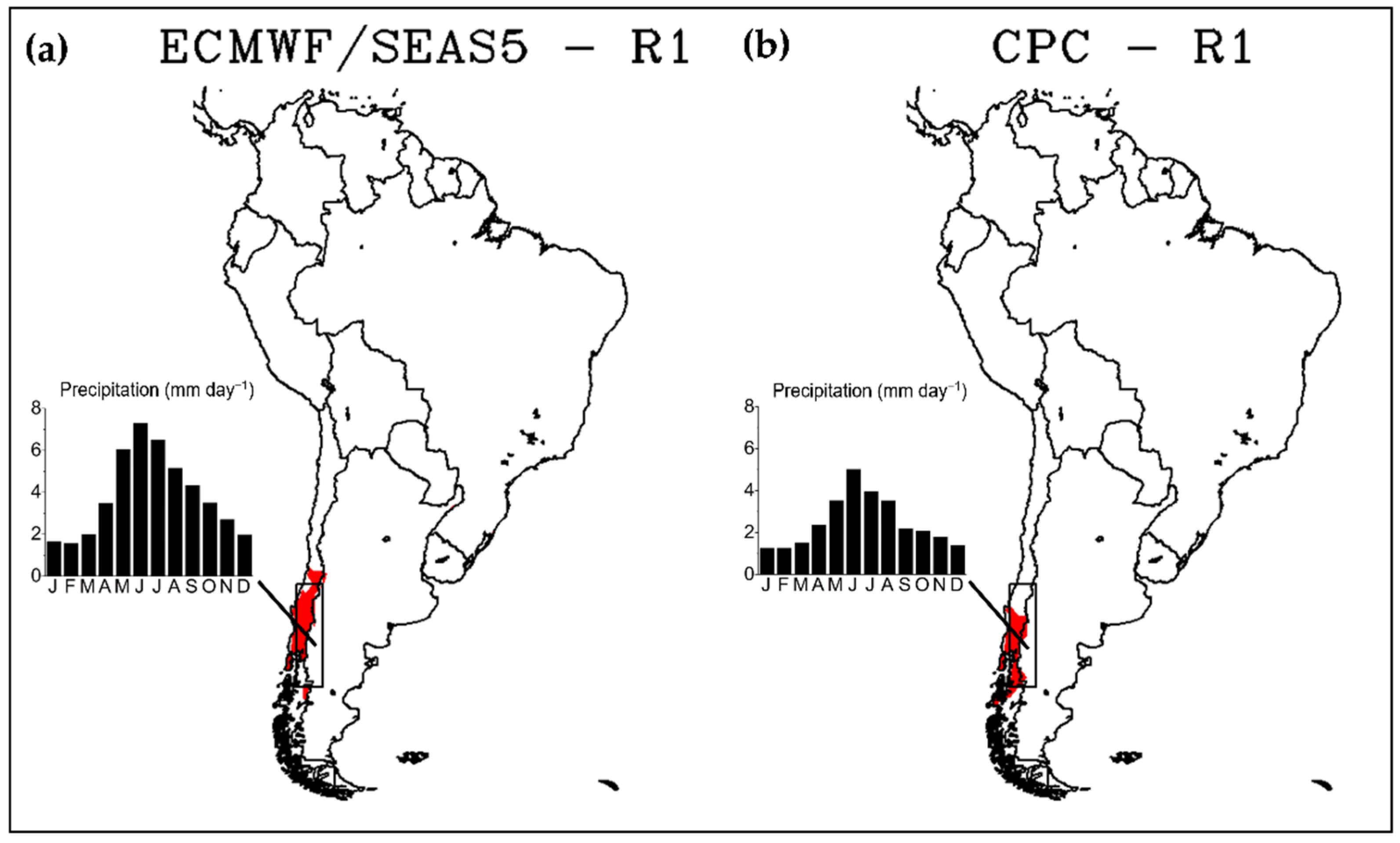
3.3.1. Cluster 1—Region 1 (R1)

Region 1 (R1), delimited by Cluster 1, comprises the sectors of south-central Chile and the far west of south-central Argentina (Figure 6). This region has an annual precipitation cycle with a maximum in winter and a minimum in summer. A crucial atmospheric system that influences precipitation in R1 is the South Pacific subtropical anticyclone (SPSA), a quasi-permanent center of high atmospheric pressure developed over the southeast Pacific Ocean as a function of the general atmospheric circulation (subsidence movement of the Hadley cell) [1,112,113].

The spatial pattern of the clusters for R1 is similar in ECMWF-SEAS5 (Figure 6a) and CPC (Figure 6b). The annual precipitation cycle (centered at 35° S–45° S and 70° W–73° W) obtained by the two datasets indicates that ECMWF-SEAS5 adequately represents the seasonal rainfall variation in the region, with maxima in the austral winter and minima in the summer, but overestimates precipitation by up to 2.5 mm day⁻¹ in the rainy season months (May to September). GCM limitations in simulating precipitation in the Andes are associated with the coarse spatial resolution, which restricts the representation of mesoscale circulation features and topographic forcing acting on the complex terrain of the mountain range [3,114]. GCMs also present a wet bias south of 35° S, mainly along the Andes mountains and southern Chile, where such models can exceed precipitation values by up to 100 mm during the rainy season in winter [70].

During austral winter, SPSA moves to lower latitudes, showing central latitude around 28° S [113], which allows the westerlies in its southernmost position to reach the Andes, being forced to ascend the topographic barrier and favoring precipitation on the western side of the mountains [113,115,116,117]. In addition, transient systems such as fronts and extratropical cyclones that move eastward embedded in the midlatitude westerlies reach R1, producing substantial precipitation in Chile’s central and southern portions [118]. An increase in the number of coastal low-level jet events (southerly winds along the west coast of subtropical SA influenced by the SPSA and essential to the coastal ocean climate) was found in the region during winter associated with changes in pressure centers and increased frequency of extratropical migratory cyclones reaching the southern coast of SA [119].

On the other hand, during austral summer, SPSA is located in its southernmost position, so the subsiding movements from the anticyclone’s southeastern flank inhibit the development of cloudiness and the passage of transient systems over R1 [1]. Furthermore, besides SPSA expanding over the Southeast Pacific, in the summer there also occurs the southward displacement (50° S–55° S) of the storm track, restricting the passage of low-pressure systems over R1 and, consequently, the occurrence of rainfall in this sector [118,120].

Low-frequency mechanisms, also called teleconnection patterns or modes of climate variability, can disrupt the annual precipitation cycle in R1. However, assessing how the climate variability (in their various timescales) impacts precipitation in R1 (and the other sectors of SA) is beyond the purposes of this work. Within this context, Reboita et al. [121] present an extensive and detailed description of the climate variability modes that most influence precipitation and atmospheric circulation in several regions of SA. Notwithstanding, studies indicate that the SPSA intensification is associated with the weakening of the Pacific Decadal Oscillation (PDO) positive phase and the strengthening of the Southern Annular Mode (SAM) positive phase in recent decades [14,121,122,123,124,125,126,127,128,129,130,131]. Furthermore, these factors are related to the reduced rainfall in Chile’s central and southern sectors [124,128,129,130]. In any case, only the natural climate variability does not justify the negative trends in precipitation. Approximately a quarter of the rainfall decrease in central Chile is due to anthropogenic forcing, which has contributed to the persistent drought in the region in recent years [129].

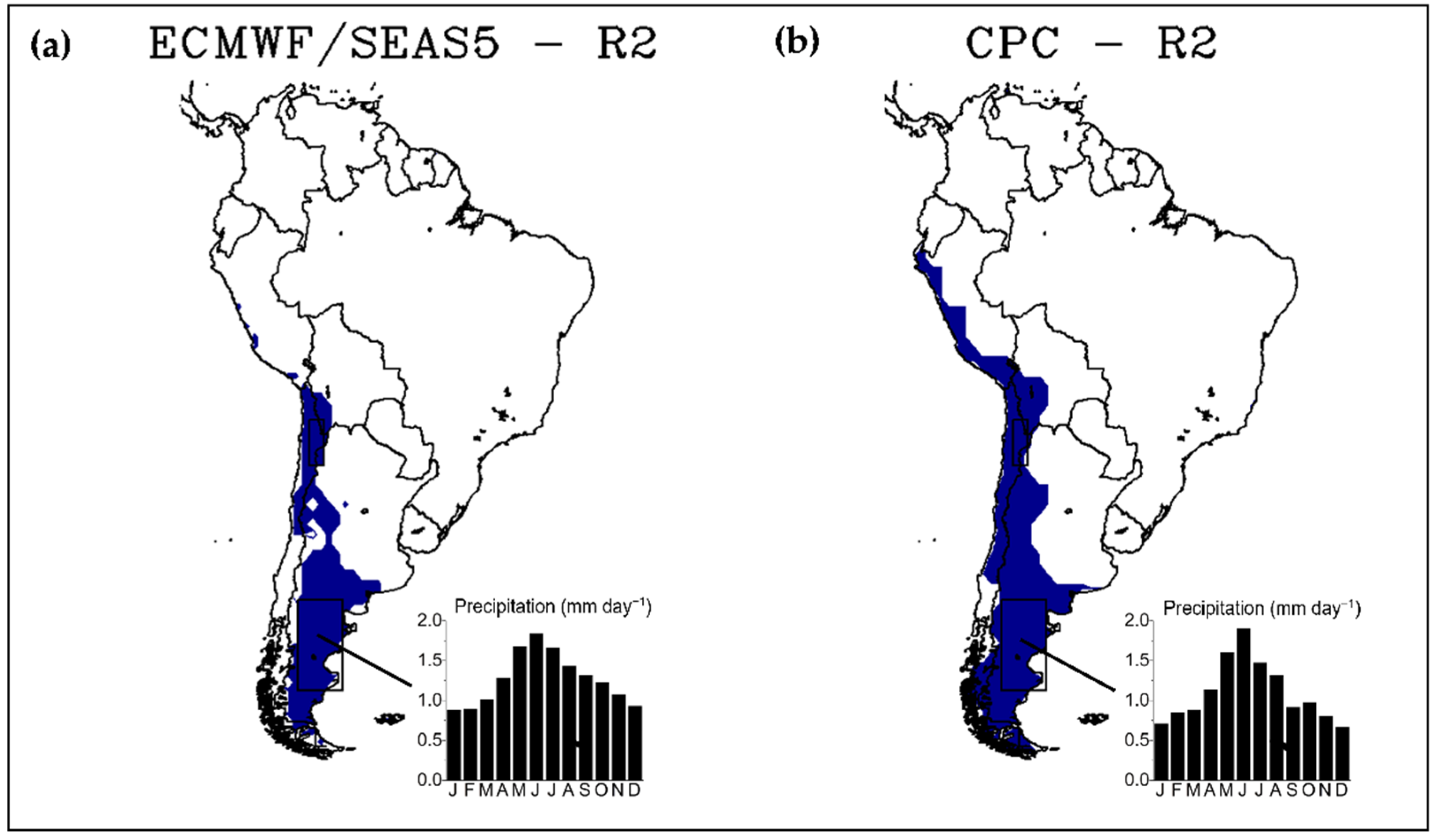
3.3.2. Cluster 2—Region 2 (R2)

Region 2 (R2), provided by Cluster 2, is formed by northern Chile and south-central and northwestern Argentina. Despite its considerable meridional extent (20° S–55° S), R2 has a similar annual cycle with low rainfall [1].

The spatial distribution of the clusters (Figure 7) has some differences between CPC and ECMWF-SEAS5. The CPC cluster comprises areas of south-central Chile, southwestern Bolivia, and the entire coast of Peru that ECMWF-SEAS5 does not include. Considering southern Argentina (centered on 45° S–50° S and 66° W–72° W), ECMWF-SEAS5 appropriately simulates the annual cycle of precipitation, with rainfall maxima from May to August, although it has a slight overestimation from September to December.

Regardless of its latitudinal extension, R2 presents low rainfall totals; different mechanisms acting in the northern and southern zones justify the slight precipitation in the region [1]. In the R2 northern portion, subsiding movements of SPSA restrict the occurrence of convection and rain in the Andean Altiplano’s western sector, propitiating one of the world’s driest areas, the Atacama Desert, which covers portions of Chile, Argentina, Bolivia, and Peru [30,31,84]. However, factors other than the SPSA’s subsidence act on the configuration of the Atacama aridity, including local features, such as the steep coastal topography, adjacent cold ocean, and local descending circulations forced by the warming of the Andean slopes [131]. Additionally, modeling studies that reduce the Andes’ height do not indicate wetter conditions over the Atacama, which continues under strong subsidence and the action of dry and cold air from the Pacific [115]. Conversely, the region east of the Andes is influenced by the moist and warm easterly winds from the Amazon Basin that feed convective storms during austral summer [84,117,123].

Despite its hyperaridity, heavy precipitation events have occurred in several areas of the Atacama Desert. According to Veloso [132], these events are associated with at least three distinct patterns: cold fronts, subtropical cutoff lows (COLs), and summer monsoon. COLs are synoptic-scale systems formed when a high-level trough amplifies towards subtropical latitudes so that a cyclonic anomaly disaggregates from the extratropical westerlies [133]. COLs are relevant in R2 [134,135,136,137] since they are responsible for up to 30% of the annual precipitation in northern Chile, contributing to annual rainfall averages of up to 50 mm in the northern semiarid region, besides having the ability to produce localized and intense events [118].

Although COLs favor the occurrence of rain in an arid and stable region, they can also cause floods, material damage, and human losses. An impressive example occurred in March 2015, in which a COL was responsible for one of the most impactful natural disasters in Chile, with rainfall accumulations of up to 100 mm over three days, floods that destroyed several cities, billions of dollars in economic damage, and the deaths of 50 people [118,132].

Southern R2 comprises the south-central and southwestern sectors of Argentina. Since this region is located leeward of the Andes, the westerlies that cross the mountain range arrive with little moisture at the eastern side, given that topography induces precipitation windward of the Andes in R1 [1,116,117]. Therefore, rainfall in this sector is mainly due to frontal and cyclonic systems that cross the region in its southern portion [1].

Southern R2 is a frontogenesis region due to different factors, such as the incursion of cold air masses that move from the South Pole to lower latitudes and the confluence of currents from Brazil (warm current) and Malvinas (cold current) [1,115]. During autumn and winter, the weakening and northward displacement of the SPSA allows greater passage of frontal systems originating from the Pacific Ocean, contributing to an increase in rainfall of up to 65 mm in this sector of R2 [138]. The southern region of Argentina (35° S–45° S) has a maximum frontal frequency in all seasons, with an annual average of 51–61 cold fronts [139]. In addition, synoptic chart analyses and objective tracking indicated an annual (seasonal) average of approximately 100 (24) cold front passages at Rio Gallegos, in the south of Argentina (51° S–69° W) [140].

The southeast coast of Argentina (45° S–50° S) is also considered a cyclogenetic zone [141,142,143,144,145,146,147], with an average incidence of 62 cyclogeneses per year (the result was computed by a cyclone tracking algorithm through cyclonic relative vorticity) [146]. This feature results from the regeneration of systems moving from west to east after crossing the Andes and high-level troughs arising from the baroclinic instability of the westerlies [141,142,143,144,145,146,147]. The jet stream position and occurrence of potential vorticity streamers also contribute to a more baroclinic environment in the region, especially in the summer [147].

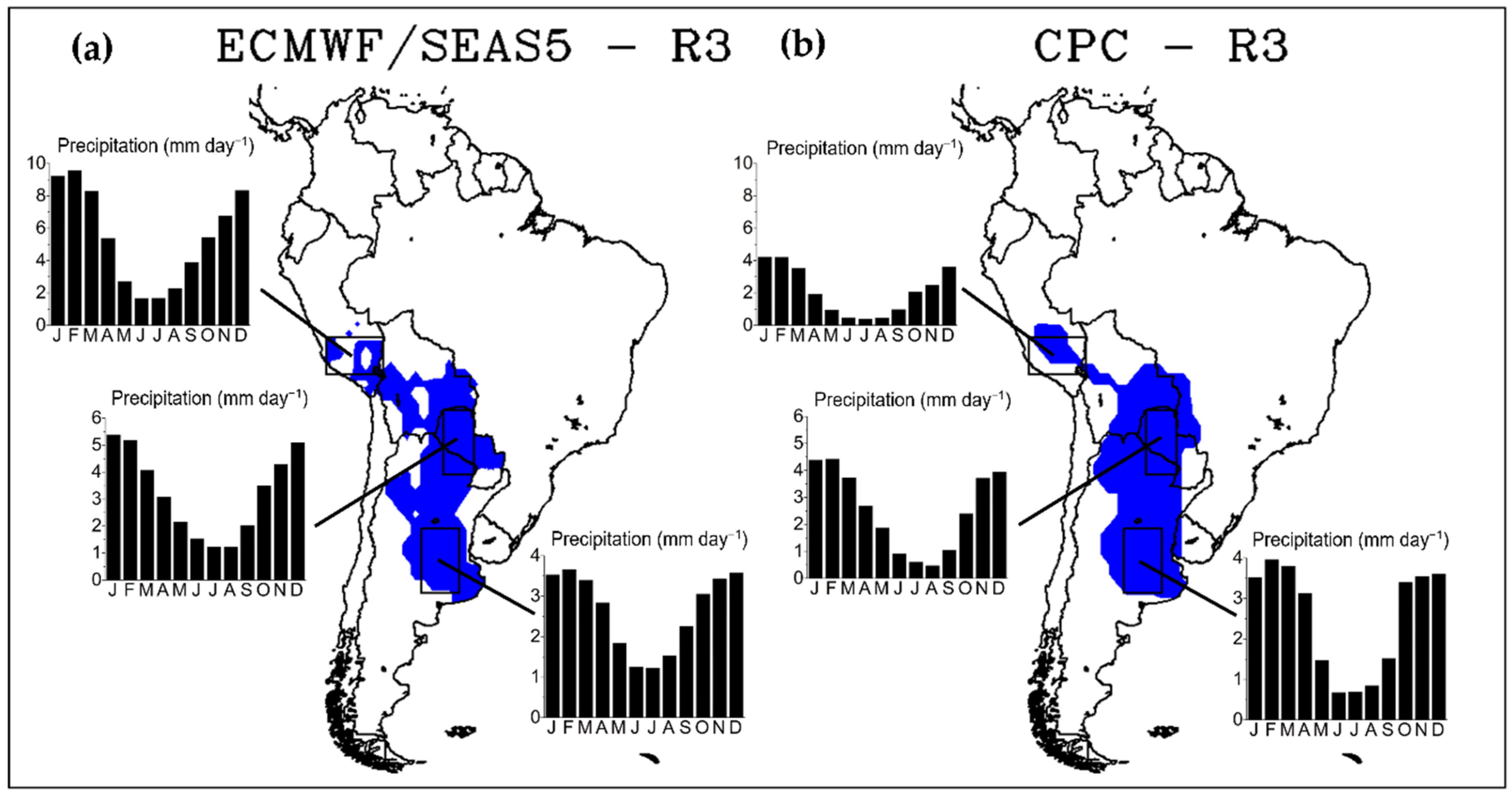
3.3.3. Cluster 3—Region R3 (R3)

Region 3 (R3), provided by Cluster 3, groups the sectors of southwestern Peru, western/southern Bolivia, central–northern Paraguay, and northern/central–eastern Argentina. This portion of SA has its annual cycle of precipitation typical of a monsoon, with two well-defined seasons, characterized by a higher rainfall in the summer and lower rainfall in the winter [1]. However, SACZ does not act in R3, and the region registers lower precipitation values than those recorded in central SA and Southeastern Brazil [1]. In the summer, the intense heating of the earth’s surface resulting from the availability of solar energy favors convective development throughout the R3. Moreover, this region receives moisture and warm air from tropical latitudes by SALLJ mainly in the summer, which justifies the maximum rainfall recorded in this season [1].

Although the clusters obtained by the two datasets indicate similar spatial distributions, ECMWF-SEAS5 has a more fragmented distribution to the east of the subtropical Andes (Figure 8a).

At the northern R3 (centered at 18° S–25° S and 58° W–62° W), ECMWF-SEAS5 simulates the phase of the seasonal precipitation cycle similar to CPC but overestimates monthly precipitation totals throughout the year, presenting an annual mean up to 2.5 times higher than CPC. The coarse spatial resolutions of the GCMs limit their ability to simulate precipitation, particularly over the eastern Andes and the Andes–Amazon transition zone [114]. Physical processes related to the complex topography of the Andes are still too smoothed in global models, so a more refined resolution (2–20 km) is required for better representing the Andean topography and simulating the orography–atmosphere and land–atmosphere interactions [3,114]. In addition, simulated precipitation in this region is poorly validated due to the scarcity of rain gauges in the region and the precipitation estimate limitations by satellites [3,148,149]. In this scenario, the low densities of stations and measurements on complex terrain restrict data acquisitions for model validation and may lead to misinterpretation of performance [150].

ECMWF-SEAS5 simulates the annual precipitation cycle phase in the central and southern sectors of R3 (Figure 8a) and minor discrepancies between the predicted and observed precipitation compared with the annual cycle obtained in the northern R3. For the center of R3 (coordinates 31° S–38° S and 60° W–65° W, located in the north-central part of the La Plata Basin—LPB), simulations indicate an adequate representation of the annual cycle of rainfall, with higher (lower) volumes in the summer (winter). However, ECMWF-SEAS5 overestimates precipitation throughout the year, with larger biases in the spring and summer months. Studies relate the wet behavior of GCMs in this region of SA [151,152], which stems from their coarse resolution and misrepresentation of the steep terrain and the large zonal gradients of topography between the Equator and 40° S [151]. Despite moderately simulating the grid–scale interaction of moisture and dynamics, GCMs are less suitable for representing intense precipitation originating from frontal systems at extratropical and subtropical latitudes [152,153].

The essential role of SALLJ in moisture transport to the south of LPB in austral summer [154] is also a critical issue for GCMs, as the models’ simulations of low-level circulation indicate they underestimate the northerly flow and its transport of warm and moist air to the southeast of SA, which is reflected in lower precipitation estimates [152]. Such bias is evident in the annual cycle derived from ECMWF-SEAS5 for the southernmost sector of R3, showing lower volumes of rainfall from October to March (Figure 8a).

In particular, the region east of the Andes in Peru and Bolivia records some of the highest orographic precipitation values in the world, especially during the summer [155], and has one of SA’s lightning hotspots, Chimoré, Bolivia [156]. Nonetheless, a part of these winds moves towards the subtropics with speeds greater than 12 ms⁻¹, configuring the SALLJ and transporting moisture to regions of Bolivia, Paraguay, south-central Brazil, Uruguay, and Argentina [1,2,61,62,154]. Researchers have found an increase in frequency, intensity, and moisture flux by SALLJ in most seasons during the last decades, impacting precipitation in sectors of SA, such as the R3 and southeastern region of Brazil [157,158]. In the LPB region, SALLJ modulates precipitation producing rainfall volumes 32% greater than events without SALLJ participation [153].

SALLJ also favors the development of mesoscale convective systems (MCSs) over the R3 territory. MCSs are characterized by an agglomerate of convective clouds that present an area with continuous precipitation, which may have various forms, such as partially stratiform or partially convective [159]. Subtropical MCSs in SA are larger and have a longer lifetime than those found in North America, around 14 h [160], and occur on about 41% of days with SALLJ activity [161]. The south-central part of R3—which includes northern Argentina, northwestern Paraguay, and southern Bolivia, comprising portions of LPB—has its spring and summer rainfall variability strongly related to MCSs [162]. Furthermore, central R3 is a hotspot for MCSs, where they contribute to more than 40% of the rainfall in the warm season, besides being associated with severe events [14,162,163]. Indeed, the region is known for some of the most intense storms ever recorded [164].

Additionally, southeastern R3 is located near a cyclogenesis hotspot, around 35°S in Uruguay [141,142,143,144,145,146]. Some aspects contributing to this feature include the westerlies’ baroclinic instability, subtropical COLs crossing the continent, the lee effect induced by the Andes, and moisture transport from Amazon by SALLJ [141,143]. As a result, this region provides an annual average of 37 cyclogeneses, although GCMs may underestimate this number because they are less suitable for simulating cyclogeneses associated with diabatic heating of moisture convection and local circulation processes, such as air–sea interactions [146].

Frontal systems also impact R3. In the locality of Bahía Blanca (38° S–62° W), on the southeast coast of Argentina, an annual average of 70 cold front passages was identified through synoptic charts [140]. The frequency of these systems diminishes as the latitude decreases.

A peculiar climate feature in R3 is the northwestern Argentinean low (NAL), characterized by a thermal–orographic low-pressure over northwestern Argentina [60,165,166,167]. Datasets with coarse horizontal resolutions commonly connect NAL with the Chaco low (CL), showing an erroneously unique thermal low. However, NAL is distinct from CL in several aspects related to its dynamic and thermodynamic structure [60]. NAL is a depression of a thermal–orographic origin, marked by the heating of the low/middle troposphere promoted by the superficial fluxes of sensible heat; thus, a quasi-permanent system during summer [60]. In addition, NAL can have intermittent activity in the winter when its genesis has a more baroclinic origin, caused by the adiabatic compression of subsidence movements leeward of the Andes, associated with the displacement of a COL from the Pacific to the Atlantic Ocean [60,167]. NAL and CL create low-level pressure gradients with tropical latitudes favoring the SALLJ displacement to R3.

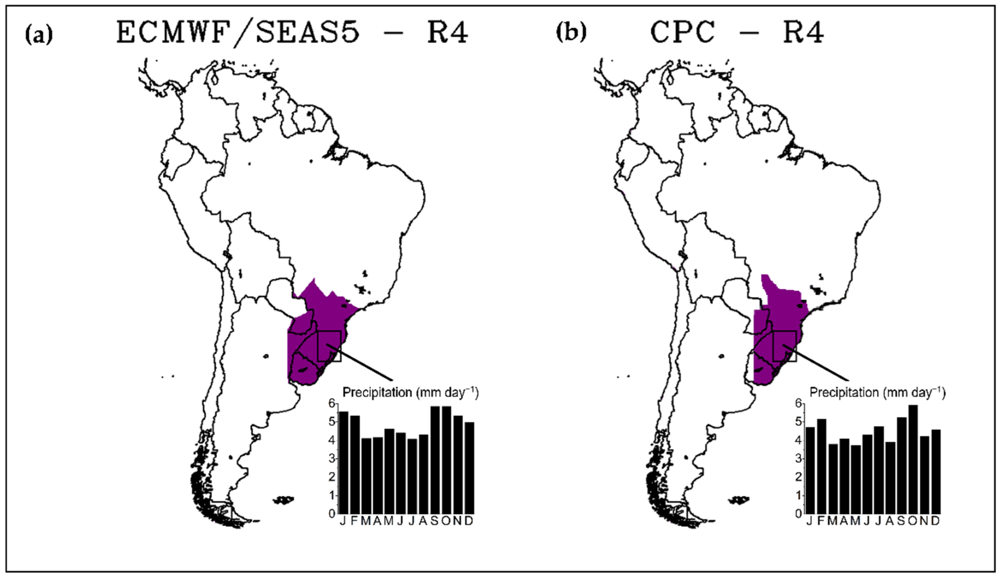
3.3.4. Cluster 4—Region 4 (R4)

Region 4 (R4), delimited by Cluster 4, encompasses Uruguay, southern Paraguay, and southern Brazil (Figure 9). This area locates between the tropics and middle latitudes, favoring contrasts in its climate regime. R4 has well-distributed precipitation throughout the year, with higher rainfall totals on the southwest border of Brazil and Paraguay [1].

The spatial pattern of the clusters obtained by the two datasets (centered at 27° S–31.5° S and 50° W–53.5° W) shows a slight difference since the area is more expanded northward in ECMWF-SEAS5. Moreover, many atmospheric systems that act on R3 also occur in R4, so it is suggested that the model biases are due to previously mentioned issues. These aspects include the deficiency in simulating the precipitation from frontal systems and orographic processes, misrepresentation of physical processes involved in developing convective conglomerates, limitations in the reproduction of the cyclogenesis associated with diabatic processes and air–sea interactions, and underestimation of the moisture flux promoted by SALLJ, among other points.

During austral winter, there is an increasing latitudinal gradient of temperature, enhancing the baroclinic instability and promoting cyclogenesis and greater penetration of cold fronts in the southern R4, which explains its considerable rainfall in the cold season [1,138,168,169]. Therefore, cold fronts are crucial systems in R4, as they contribute substantially to the rainfall totals and are associated with more severe conditions such as strong winds and intense precipitation [169,170].

Diverse methodologies of cold front detection provide different results. For instance, studies with tracking algorithms using observed data and reanalyses indicate an average of 55 cold fronts per year [169] and seasonal averages of 11 and 13 cold fronts in the winter and spring, respectively [139]. On the other hand, analyses of cold front incursions in southern R4 using synoptic charts result in an average of 43 to 48 cold fronts per year in Porto Alegre, southern Brazil [140,168], with seasonal averages of 14 and 12 occurrences in the winter and spring, respectively [140].

In R4, there are also frequent cyclones (mainly in the winter and spring) since the region is surrounded by two cyclogenetic hotspots to the south and east [1,141,142,143,144,145,146]. Several aspects propitiate cyclogenesis in R4. Among these factors, there are baroclinic waves from the westerlies penetrating in subtropical latitudes [141,142,143,144,145,146], the presence of COLs that form over (or enter) the region [142,147], the Andes contributing to the lee cyclogenesis [142], advection of warm and moist air from the Amazon by SALLJ [144], enhancement of baroclinic instability by the strong SST gradient caused by the confluence of the Malvinas current (cold) with the Brazil current (warm) [145], advection of heat and moisture by the SASA northerly flow [144], the influence of the upper-level subtropical jet, and potential vorticity streamers [147].

The cyclogenesis identification by objective methods indicates an annual average of 37 cyclogeneses south of R4 [146], with a higher frequency in May, approximately 27 cyclogeneses [142], and in the austral winter, with a seasonal average of 11 cyclogeneses [145]. According to Reboita et al. [142], the most regular seasons for cyclogenesis in SA are the summer in southern and southeastern Brazil and the winter in the LPB, which reiterates previous results [141]. It is emphasized that these values are dependent on the methodology used, including data sources, model types, period and domain of the analysis, and detection method. Regardless, it is stressed that GCMs may underestimate these values since many cyclogeneses in the region develop through diabatic processes and local circulation, which are not always well captured by the models, being more appropriate for using dynamical downscaling with regional models [142,146].

The cyclogenetic region more to the northeast of R4 [142] registers an annual average of 26 cyclogeneses [146], a seasonal average of 7 cases in the summer [145], and a higher frequency in December [142]. Reboita et al. [171] verified a positive trend of cyclone occurrence in R4 (on the coast of Uruguay) for the period 1980–2012, as well as a projection of increased cyclogenetic activity in the near (2020–2050) and far (2070–2099) futures [172,173], besides a positive trend of explosive extratropical cyclones, which form mainly on the coast of Uruguay and are associated with extreme winds and severe precipitation [174]. According to the authors, the increase in cyclogenetic activity near Uruguay may be a consequence of the intensification of the subtropical jet at upper levels and the moisture input at lower levels promoted by anomalous northeast–easterly winds from the South Atlantic Ocean [173].

MCSs are also mechanisms for precipitation all over the R4. MCSs acting in R4 have peculiarities concerning those found in other subtropical regions of SA. MCSs in R4 last longer (+3 h) and are 50,000 km² larger [175], besides having as sources of moisture for their genesis both the vapor transported by SALLJ and that advected by the SASA northern flow [159,160,161,162,163,175,176,177,178]. During the winter, MCSs can form with the passage of frontal systems in the region, as the propagation and intensification of convection occur along cold fronts, contributing to MCSs development [176].

Subtropical COLs are also atmospheric systems with notable action in R4. Studies show that the southeast of SA (including portions of the R4 such as Uruguay and southern Brazil) is the region with the highest frequency of these systems when considering the entire continent and adjacent oceans [133,134,135,136,137,147,179,180,181]. Besides propitiating the formation of cyclones, COLs are relevant in R4 because, depending on their positions, they can contribute to rainy or dry conditions in the region [1].

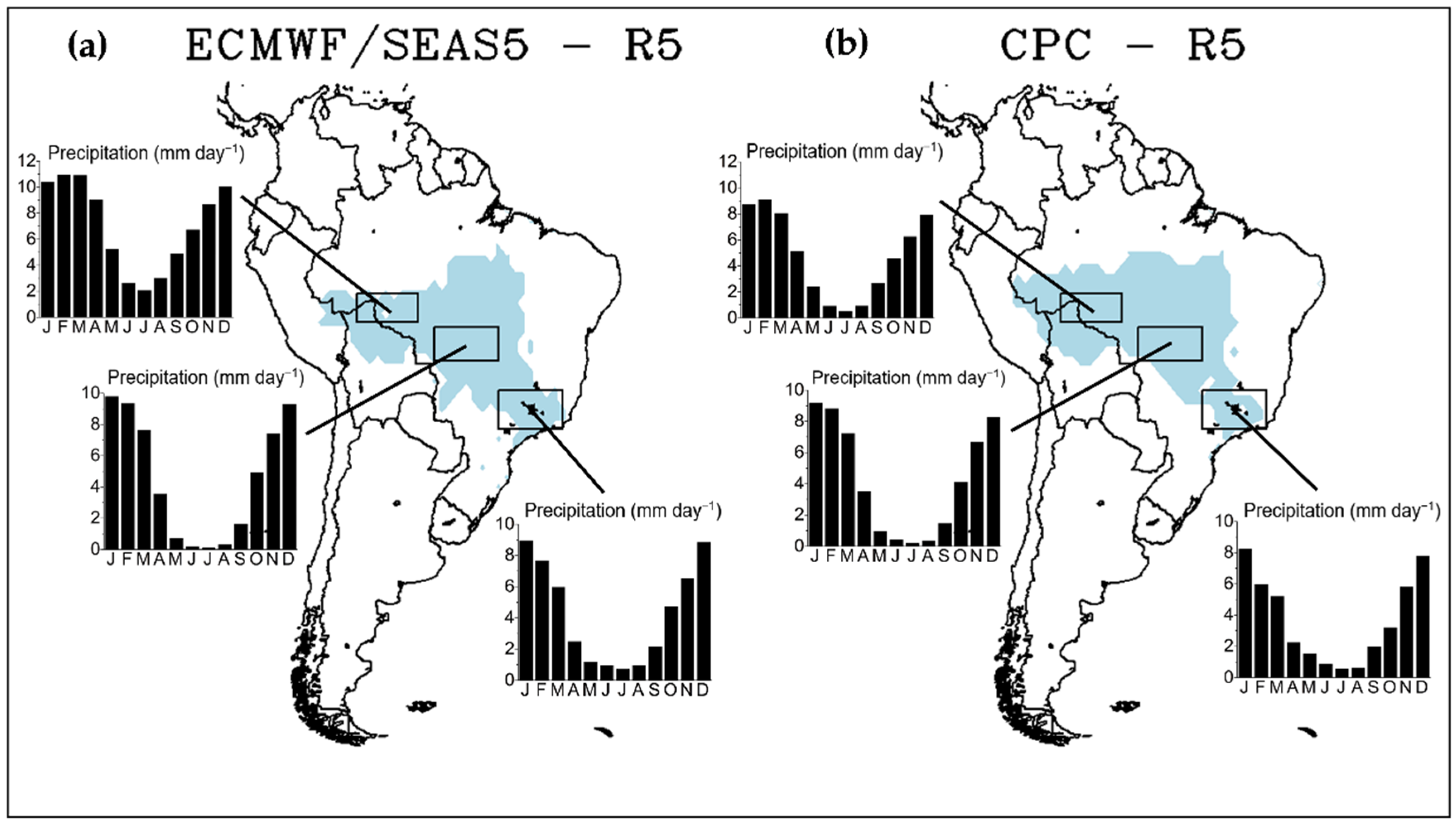
3.3.5. Cluster 5—Region 5 (R5)

Region 5 (R5), delimited by Cluster 5, comprises a broad territory that extends from the south of the Brazilian Amazon to southeastern Brazil, passing through central–western Brazil and northern Bolivia (Figure 10). In this sector, the maximum rainfall occurs in the summer and the minimum in winter. Therefore, both clusters show a similar spatial distribution and comprise the central regions of SA with maximum rainfall during the summer, as illustrated in Figure 10a,b. Furthermore, the spatial distribution from the two datasets resembles the SA portion where SACZ is most influential, as described in Section 3.2. So, this is the typical monsoon area of SA [51].

The annual rainfall cycle of ECMWF-SEAS5 in Southeastern Brazil—SEB (centered at 19° S–23° S and 42° W–50° W)—is similar to CPC, although with a wet bias throughout the year with larger overestimates in October and February. However, the model’s ability to represent regional rainfall is noteworthy, considering that this R5 sector is inserted in a spatial range of low climate predictability, given its variety and variability of atmospheric systems and their transient nature [182].

SACZ plays a pivotal role in the SEB rainy season. However, one of the major SACZ consequences in SEB is the effect of heavy rainfall, causing natural disasters in the region. For example, SACZ is related to about 47% of the SEB natural disasters with intense precipitation between 1960 and 2005 [183]. Therefore, a natural disaster in the SEB has a 24% chance of occurring in the SACZ presence, with higher chances of SACZ disasters in the states of Espírito Santo and Minas Gerais [184]. Generally, in the São Paulo and Rio de Janeiro regions, other systems concomitant to SACZ, such as cold fronts, are associated with natural hazards [185,186].

For instance, in the state of São Paulo, 35% of extreme precipitation events were associated with the SACZ presence [37], while for Rio de Janeiro, 48% of SACZ events cause intense precipitation in the region [187]. Moreover, over Rio de Janeiro, a well-configured cyclone on the southeast Atlantic coast was associated with SACZ during extreme events [187], a condition similarly verified by Reboita et al. [188] when there were occurring disasters in southern Minas Gerais. Recently, extreme precipitation from SACZ caused some of the deadliest natural disasters in Minas Gerais [189] and Petrópolis (Rio de Janeiro state) [190], causing more than 200 deaths and thousands of homeless.

Cold fronts are also relevant in natural disasters over SEB, being associated with 53% of the extreme precipitation events in the region [183] and up to 47% of these events in the state of Rio de Janeiro [191]. The identification of cold fronts by an automatic method resulted in a seasonal average of five to nine cases in the winter and spring [139]. Additionally, synoptic charts give annual averages of approximately 24 [140] and 25 [168] cold fronts in the region. Conjointly, the localities of São Paulo and Rio de Janeiro record the highest occurrences of baroclinic troughs, about 11 systems per year, which distinguish themselves from classical cold fronts by presenting cloudiness, precipitation ahead of the system, and weak horizontal temperature gradient [168]. Despite being more frequent in the rainy season, baroclinic troughs also affect SEB at the end of the dry season and are responsible for about 40% (60%) of the rainfall in the rainy (dry) season in SEB [168].

During the winter, the low rainfall totals relate to SASA being zonally extended, reaching its westernmost position, with establishment mainly over the SEB [63]. Under the SASA in winter, SEB experiences weather with clear skies, weak winds, and subsidence movements, the blocking of the synoptic system’s passage and inhibition of cloud formation, and developing thermal inversions in the atmosphere. All these conditions are unfavorable to the dispersion of pollutants in the most urbanized Brazilian region [192,193].

Regarding the metropolitan region of Rio de Janeiro, about 88% of the days in which particulate matter (PM₁₀) concentrations violate air quality standards have the SASA presence over the sector, and 60% of these days occur from May to September [194]. For the metropolitan region of São Paulo, the maximum concentrations of ozone (O₃) and PM₁₀ are also associated with the SASA well-configured over the SEB, generally from April to October [195]. In this period, precipitation usually occurs when frontal systems and subtropical/extratropical cyclones surpass the SASA, besides other atmospheric systems, such as MCSs, breezes, and atmospheric blockings [1]. Still, on air pollution in the SEB, the sea and land breezes have a fundamental role in contributing to the dispersion of pollutants from the metropolitan regions [196].

It was believed that the Atlantic Ocean basin is a climatologically unfavorable environment for developing tropical cyclones due to its strong vertical wind shear and cold SST [197]. Nonetheless, in March 2019, the first purely tropical cyclone (since the satellite era) was recorded, named Iba; its synoptic and meteorological attributes were analyzed by Reboita et al. [198]. The authors found that the cyclogenesis possessed typically tropical characteristics, such as weak vertical wind shear and warmer SST. In addition, Iba presented high precipitation associated with the SEB coast, such as approximately 62 mm on March 22 at the São Mateus station in Espírito Santo. Furthermore, Silva and Reboita [199] evaluated the potential for tropical cyclogenesis in the Atlantic Ocean; their results indicate that there are potential conditions conducive to the formation of tropical cyclones in the region, mainly along the coast of Bahia and Espírito Santo, with maximum intensity between February and March, when it also reaches the southern coast of Brazil (R4).

The annual cycle of rainfall from ECMWF-SEAS5 in Midwestern Brazil (MWB)—centered at 12.5° S–16° S and 50° W–58° W—represents well the seasonal rainfall pattern, despite overestimating (underestimating) in August through December (May and June). Nevertheless, the model’s performance in representing rainfall in a region of low climate predictability [182] is notable.

Some cold fronts with large meridional displacement can contribute to the incursion of cold air into the tropics, affecting the Amazon and the local population with a substantial reduction in air temperature and humidity, a phenomenon known as “friagens” [1,200,201,202]. Although they are more associated with the Amazon in the literature [200], friagens can also reach the northern MWB [202]. In this sense, Escobar et al. [202] examined the frequency of friagens in the northern MWB and identified 217 cases in the 1961–2012 period.

Northern Brazil (NB) presents spatial and seasonal heterogeneity of rainfall, with maximum precipitation in the western sector [1,201]. ECMWF-SEAS5 simulates the pattern of the annual cycle in northern R5 (centered at 9° S–12° S and 60° W–67.5° W), despite its wet bias with larger deviations in the rainy months.

Local convection is an important driver of precipitation in this region. MCSs also contribute to precipitation in the NB, but their development is different from those in R4, i.e., in NB, they are driven by thermal heating of the surface, promoting moisture convergence and convection [1,203,204,205,206]. In general, MCSs are more frequent from December to July, and their development is more prominent in the afternoon and early evening, with an average speed of 14 ms⁻¹, enhanced by the sea breeze [205]. Their average coverage area is approximately 40,000 km² (with the largest MCSs possessing about 80,000 km²), an average lifetime of 3 h, and they rarely move beyond 1500 km within the coast [206]. Additionally, MCSs respond to 40% of the annual precipitation in the coastal belt from the state of Maranhão up to the Guyanas [205].

NB can eventually be reached by friagens, which decrease temperature due to a frontal system penetration in the northern Brazilian region. An average of 2.3 incursions per year is estimated over NB, with two-thirds occurring in austral winter [201]. Despite the low frequency, friagens promote intense precipitation in NB, with up to 40 mm day⁻¹ and a temperature decline of up to 2 °C in the central and southern parts [201]. Furthermore, in this cold incursion situation, the moisture flux from the south of the basin to the subtropics is reduced, increasing the convergence of moisture flow over the NB and contributing to convective activity in the region [201].

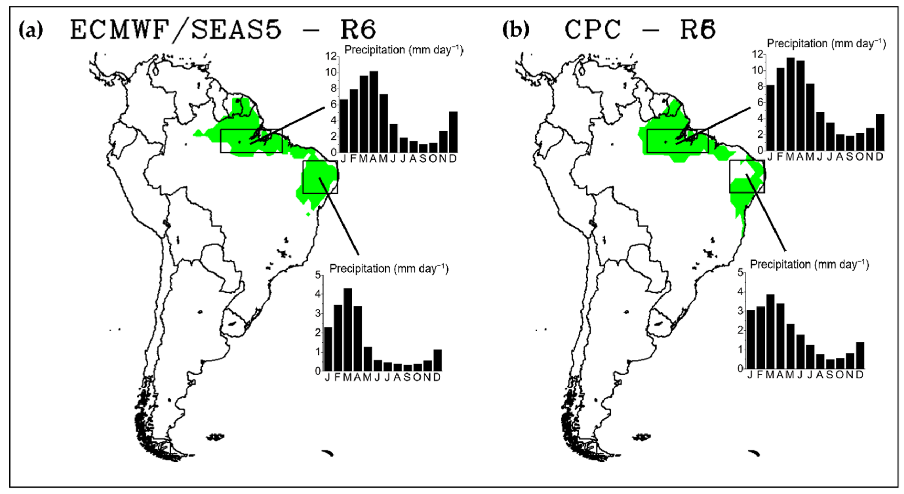
3.3.6. Cluster 6—Region 6 (R6)

Region 6 (R6), composed of Cluster 6, comprises the northern region of northern Brazil (NB) and the coast of northeastern Brazil (NEB). Figure 11 illustrates the clusters provided by the two datasets, indicating a good representation of the annual cycle of rainfall in the regions by ECMWF-SEAS5. In the northern sector of the NB (centered at 0°–4° S and 46° W–57.5° W), the model underestimates the monthly precipitation totals throughout the year. In the coastal sector of R6 (centered at 5° S–10.5 °S and 35° W–42° W), ECMWF-SEAS5 shows more evident underestimates, with larger dry biases in May through November. The system’s ability to reproduce rainfall in the first semester, especially from March to May, stands out, which may be associated with the good predictability of the strong relationship between the tropical Atlantic SST and rainfall over the NEB in this period [121,207,208,209,210,211].

ITCZ is the most relevant atmospheric system in the northern NEB and semiarid region. In the rainy season between February and May, ITCZ is in its southernmost position, around 4° S, thus being the primary dynamic mechanism responsible for the rainfall [1,207,208,209,210,211,212]. However, ITCZ migrates northward in the other seasons, and its southernmost descending branch reaches R6, inhibiting precipitation in the sector [1].

Radiative heating is also crucial for convective activity at R6 [1]. In this process, convective activity can enhance the development of tropical MCSs, which are responsible for intense precipitation in R6 [1,205,213]. MCSs form themselves mainly at night (between 19 UTC and 03 UTC), with an average total area of 120,000 km²; about 83% of the cases happened over the continent, which is justified by the major influence of synoptic systems over the continental region [213]. Likewise, the higher occurrence of MCSs in the warmer seasons is associated with the ITCZ displacement to the south of its climatological position, so the large-scale system acts as a driving mechanism for the formation of mesoscale systems [214].

Since R6 has a large coastal strip, sea breezes in the region are frequent [1]. Under these conditions, the sea breeze transports moisture to the R6 inland, which interacts with the trade winds producing squall lines that enter the continent [1,215,216,217]. Squall lines are MCSs that begin their formation north of the R6 in the late afternoon or early evening when convective cells agglomerate, forming a linear band of clouds parallel to the coast [216]. Squall lines occur all year round but have a maximum frequency in the autumn when ITCZ reaches its southernmost position, directly affecting the instability conditions in the northern R6 [216]. In general, squall lines can contribute up to 45% of the precipitation during the rainy season in eastern Pará state (northern sector of the R6) [203].

Germano et al. [217] evaluated the occurrences of sea, land, and river breezes in the northern R6 and observed that sea breeze is more frequent in the austral spring, while land breeze is more present in the autumn. A higher frequency of sea breeze in the spring is favored by the enhanced SASA northern flow that contributes to the breeze penetration perpendicular to the coast. On the other hand, the land breeze is propitiated by the maximum displacement of the ITCZ to the south during autumn so that its intense convection attenuates the mean flow, reducing the intensity of the winds that enter the coast, and favoring the land breeze incursion [217]. Regarding the diurnal cycle, the sea breezes occur more in the period 09 UTC to 21 UTC, while the land breezes are more frequent in the period 00 UTC to 09 UTC [217].

On the east coast of R6, other atmospheric systems, such as fronts, easterly wave disturbances (EWDs), and tropical COLs, also act [1]. For example, EWDs are disturbances with a quasi-periodic behavior of 3–5 days and wavelengths between 2000 and 4000 km that reach the eastern NEB coast and have an associated development over the tropical South Atlantic Ocean [1,218,219,220,221,222]. Climatological analysis of EWDs indicated 518 occurrences of the system (for 1989–2009), most frequently between April and August, of which 97% reached the coast of R6, and 64% were naturally convective [220]. The evaluation of the associated synoptic patterns showed that the primary systems originating the EWDs are cold fronts (72%), the west coast of Africa (10%), the ITCZ (6.3%), and tropical COLs (1.5%), as well as the interaction of the ITCZ with cold fronts (3%) [220].

Tropical COLs form around R6 between mid-spring and autumn, when the atmospheric conditions of SA are characterized by the well-configured BH and the presence of a trough in the NEB (Northeast Trough—NT) [223]. Tropical COLs are systems that may cause wet or dry conditions on the R6, depending on their position [223,224]. Because the COL’s center is generally cloudless, the region of R6 under this portion of the vortex experiences clear sky conditions, subsidence currents, and inhibition of convective activity. In contrast, regions under the COL’s edges have conditions favorable for rising motions and convection [1,223,224,225]. Climatological analyses of tropical COLs in R6 reveal their highest frequency in the summer [224]. In addition, they have preferential movement to the west but can also exhibit erratic movement [224,225], an average lifetime of 2 to 4 days, and an average distance traveled of 2000 km [224,226]. Generally, when tropical COLs are positioned over the Atlantic Ocean, they provide rainfall in R6, but when they are more inland, depending on their positions, they may cause dry or rainy conditions in different parts of R6 [224]. There are even rarer cases of tropical COLs that manage to move as far as north Brazil [224,225].

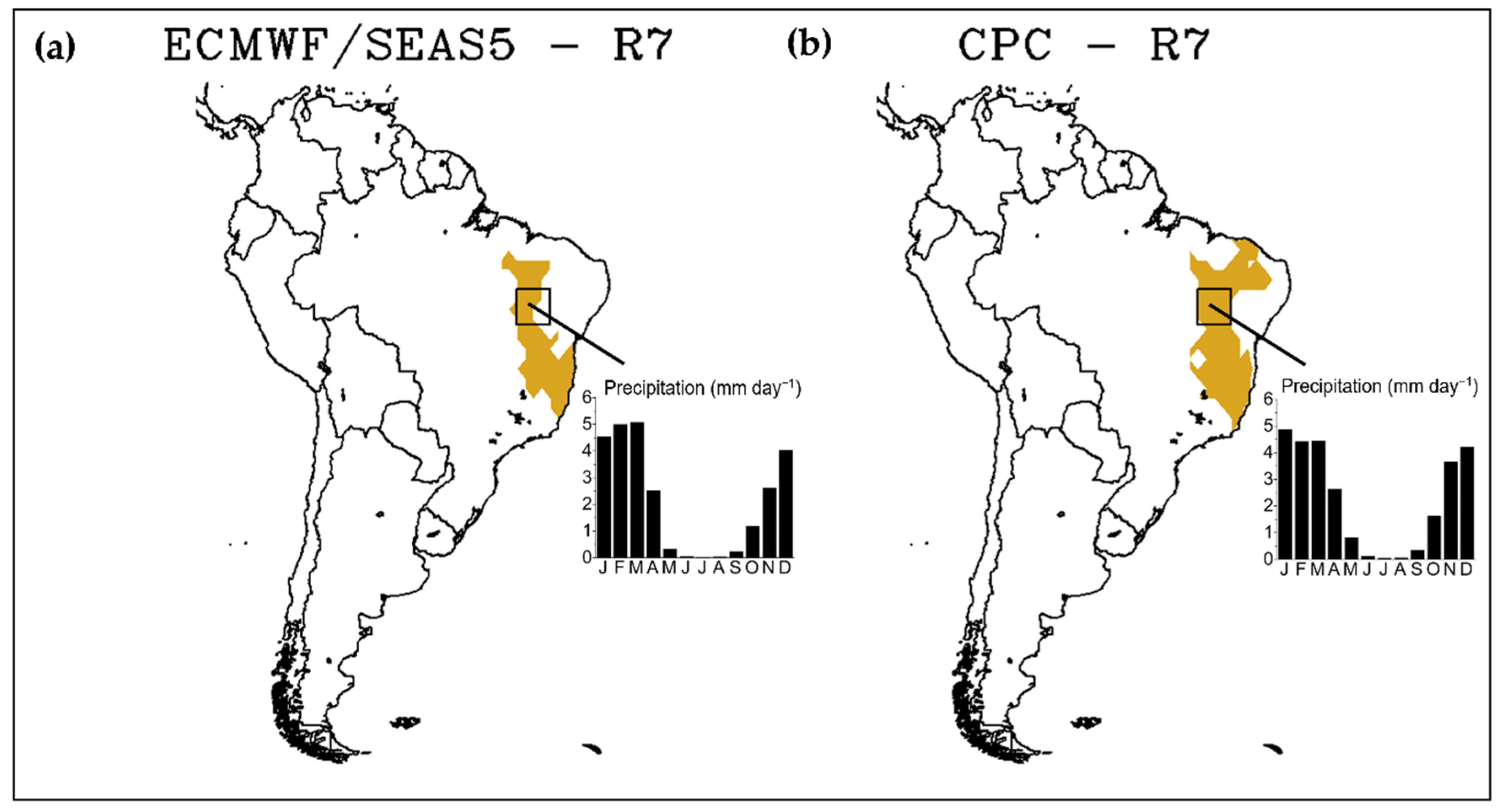
3.3.7. Cluster 7—Region 7 (R7)

Region 7 (R7), delimited by Cluster 7, includes the northeastern drylands of Brazil, a region of low rainfall totals but with an annual cycle pattern similar to R5. Considering the clusters, CPC encompasses areas of the northern NEB coast that ECMWF-SEAS5 does not group (Figure 12). However, the annual cycle of precipitation simulated by ECMWF-SEAS5 (centered at 8° S–11.5° S and 42° W–46° W) has a similar phase to CPC.

In the summer and autumn, the southward position of ITCZ favors precipitation in the region, while in winter, precipitation is inhibited by the subsidence movements of the system that is more displaced to the north [1,227,228] and also by the descending movements of the convective activity that occur in the west–northwest Amazon [1]. Besides the ITCZ, other atmospheric systems can act on R7, such as frontal systems (mainly on the coast) and tropical COLs [1,227,228].

R7 presents a remarkable interannual rainfall variability, with arid and rainy years [33,34]. Such variability is attributed to teleconnection mechanisms, such as the SST variation in the tropical Pacific and Atlantic. Additionally, during El Niño events, the subsidence cell acting on the region inhibits convective activity over the western tropical Atlantic and reduces precipitation in the NEB [32,33,34,93,207,211,228,229,230].

Reboita et al. [32] examined the causes of semiaridity in R7 through vertical profiles of the Walker and Hadley circulation cells, centered on the Borborema Plateau, to verify the topographic influence on the region’s climate. The zonal Walker circulation cell showed that the eastward flow ascends to the windward of the plateau and subsides to the leeward, promoting air heating by diabatic compression and reducing humidity on the west side of the plateau. The southern Hadley cell indicated a similar profile with air ascending to the south–southeast of the plateau and subsiding to the north, but with less intensity compared to the Walker cell. Notwithstanding, the hypothetical absence of the Borborema Plateau revealed that the temperature and moisture gradients would be less pronounced. Thus, it is inferred that subsidence downwind of the plateau couples with descending movements of the general circulation cells, intensifying the dry conditions of R7, especially in the winter [32]. Although the influence of the subsidence motions from the general circulation cells predominates over the orographic conditions of R7, it is suggested that the causes of semiaridity in R7 result from a complex interaction of regional topographic elements and large-scale dynamical mechanisms.

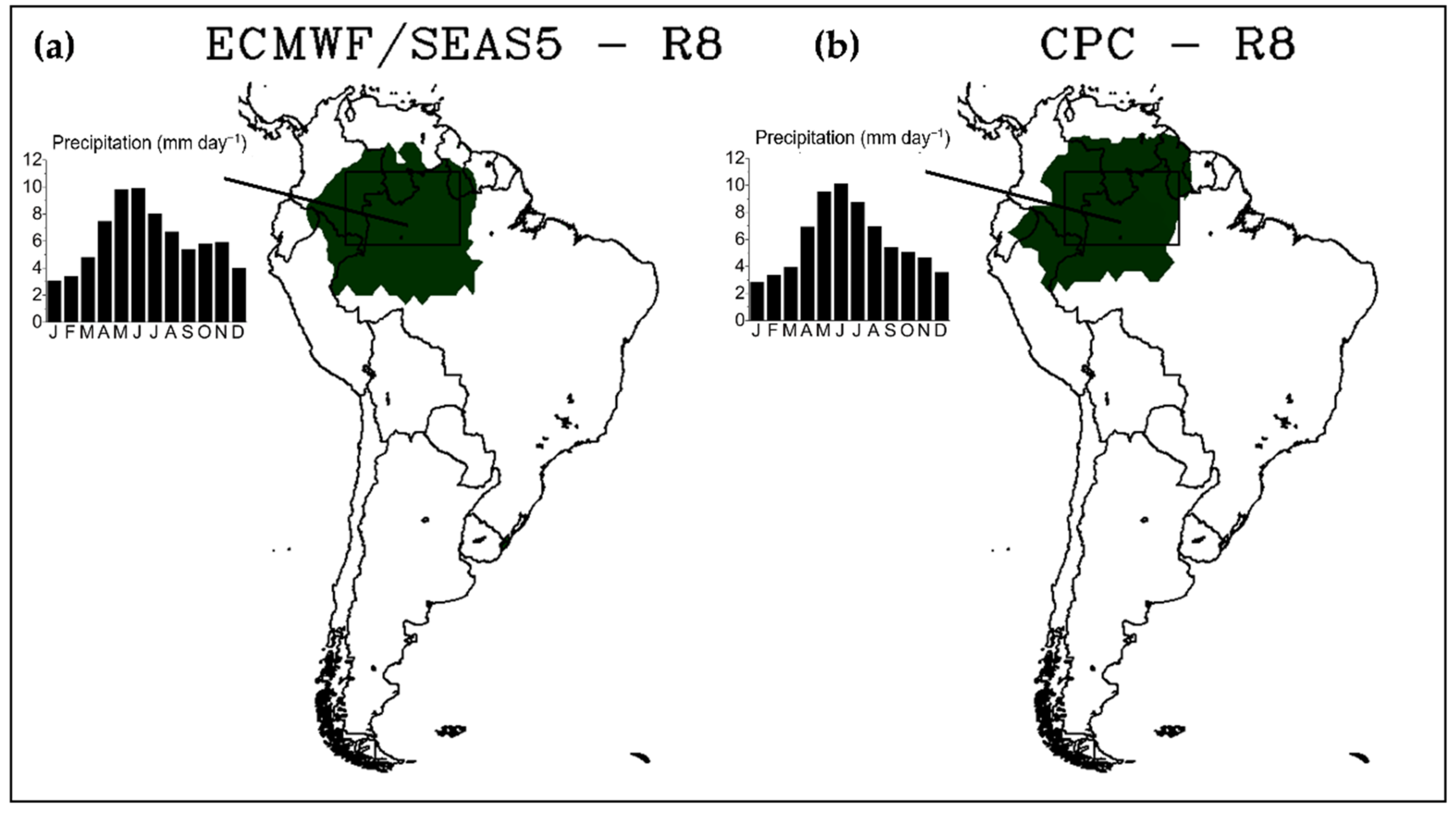
3.3.8. Cluster 8—Region 8 (R8)

Region 8 (R8), provided by Cluster 8, comprises the northern Brazilian Amazon, northeastern Peru, central–southern Colombia, and southern Venezuela. Despite the correspondence between the two clusters, the CPC cluster encompasses other sectors, such as Suriname, eastern Ecuador, and central Colombia (Figure 13b). On the other hand, the ECMWF-SEAS5 cluster has a broader extension in the southern Amazon (Figure 13a).

Moreover, ECMWF-SEAS5 also presents overestimates (underestimates) in almost the entire year (June to September), with more expressive biases in March and November. Nevertheless, it has a good performance in reproducing the annual cycle of rainfall in the region (centered at 0°–8° S and 58.5° W–73.5° W), with higher totals in May through August.

R8 also has a unique attribute: the Amazon–Andean transition region, a territory of rich biodiversity and biogeographic patterns resulting from an intricate interaction between climate contrasts and the complex Andean topography [2,231]. In this environment, the Amazon exports water vapor and nutrients to the Andes through trade winds, so these winds rise over the topographic barrier of the Andes, promoting convection, which in turn produces river runoff that transports sediments and nutrients to the Amazon rivers [2,115]. In addition, some areas of this transition region are considered rainfall hotspots (about 6000 mm year⁻¹), a consequence of the interactions between large-scale circulation and topographic features that produce enormous rainfall totals throughout the year [232].

The Atlantic Ocean and the Amazon rainforest are the primary oceanic and continental moisture sources, respectively, for most R8 (the region north of 8° S) and neighboring regions [2]. Similarly, Wang et al. [16] concluded that the tropical Atlantic contributed more than 60% to the increase in rainfall in northern Amazon between 1979 and 2015, providing an average increase of 540 mm of precipitation from December to May. On the other hand, the Amazon rainforest is the largest supplier of moisture to the tropical SA, LPB, and Andes regions [2].

Sectors exposed to the ITCZ and the Atlantic Ocean, such as the northeast and northwest of the R8 (Colombia, northern Ecuadorian Amazon, northeastern Peru, and northwestern Brazil), have more abundant rainfall (around 3000 mm year⁻¹) [233]. However, rainfall is also substantial in the southeastern portions, influenced by the SACZ [233]. Furthermore, in the Andean Amazon, there is a rainfall amplitude resulting from the precipitation reduction with altitude and different conditions on the leeward or windward sides of the mountains, recording annual totals of up to 6000 mm (below 530 mm) on the windward (leeward) side [233]. Moreover, this territory has one of the lightning hotspots in the Colombian Amazon, in Sibundoy Valley [234].

The northern sector of R8 has its annual cycle of rainfall strongly influenced by the ITCZ [1,2,3,235], with the annual maximum during autumn and early austral winter, without a well-defined dry season [232]. However, its spatial and temporal precipitation variability is due to several factors, such as the complex topography, the influence of moisture transport by the Caribbean Sea and the Pacific and Atlantic Oceans, MCSs, and synoptic disturbances, such as easterly waves (EWs) [2,3,71,235]. EWs respond to 50% of summer rainfall in northern SA [236], but 50% of their occurrences between 1983 and 2018 were associated with precipitation inhibition and clear skies [237].

The northeastern part of R8 presents maximum precipitation in the autumn, with peaks in April and May, periods of maximum interaction between the sea breeze and the trade winds generating squall lines [203,232]. Climatological analysis of squall lines in the Amazon Basin indicated that they occur on average every two days, form mainly along the northern coast of Brazil between April and June, and about half of the systems propagate up to 170 km [238].

MCSs are also relevant in R8 as they produce about 50% of the rainfall east of the central Andes [14] and a substantial share of the Amazon Basin precipitation [205]. MCSs genesis is associated with locations with high topography or near the confluence of large water bodies, such as the confluence regions of the Tapajós and Amazon rivers [239]. Rehbein et al. [239] evaluated the MCSs climatology in the Amazon Basin from 2000 to 2013 and found 7200 continental MCSs, of which 64% had short lifetimes between 3 and 6 h. Oceanic MCSs form primarily along the Brazilian coast in the northeast of the basin and have longer lifetimes (around 11 h) but occur at a lower frequency, about 50 oceanic MCSs per year [239].

4. Conclusions

The present work evaluated seasonal rainfall patterns in SA through the K-means clustering technique with CPC data and ECMWF-SEAS5 seasonal rainfall predictions. Results indicated the good ability of the European prediction system to reproduce the main climatological aspects of rainfall on the continent, including the spatial and temporal variabilities and the wet and dry seasons in different sectors of SA. In general, ECMWF-SEAS5 presented a better performance in regions with good seasonal climate predictability (such as the north and northeast of SA) due to the strong influence of the Pacific and Atlantic oceans over these areas through teleconnection patterns. Nevertheless, the system’s performance in regions of medium and low predictability was also notable, indicating that it is an appropriate tool for analyzing seasonal atmospheric patterns in SA.

Given the topographic heterogeneity and diverse atmospheric systems acting on the continent, the systematic errors of the model may be associated with the misrepresentation of regional features, such as the Andean topography and the mesoscale/local scale phenomena as the formation of convective complexes, orographic rains, and breeze circulations. In this scenario, machine learning is a promising methodology, given that seasonal predictions of precipitation for SA with the neural networks technique have resulted in up to a 75% error reduction in estimates [240].

The evaluation of the obtained homogeneous groups of precipitation allowed examining the different sectors of SA according to the atmospheric systems that act upon them and the associated precipitation cycle. In general, the most relevant synoptic systems in each region were related, but some mesoscale and local scale phenomena participating in the rainfall regimes of each sector were also discussed. Implicitly, the main physical and dynamic features that make up the precipitation patterns in each region were also described.

In addition, the results obtained corroborate the qualitative analysis of Reboita et al. [1], indicating that it is a suitable methodology for evaluating seasonal precipitation regimes in SA. Finally, this work can be used as a primary reference by undergraduate and graduate students seeking to understand the South American climate better.

References

1. Reboita, M.S.; Gan, M.A.; da Rocha, R.P.; Ambrizzi, T. Regimes de precipitação na América do Sul: Uma revisão bibliográfica. Rev. Bras. Meteorol. 2010, 25, 185–204. [Google Scholar] [CrossRef]
2. Espinoza, J.C.; Garreaud, R.; Poveda, G.; Arias, P.A.; Molina-Carpio, J.; Masiokas, M.; Viale, M.; Scaff, L. Hydroclimate of the Andes part I: Main climatic features. Front. Earth Sci. 2020, 8, 64. [Google Scholar] [CrossRef] [Green Version]
3. Arias, P.A.; Garreaud, R.; Poveda, G.; Espinoza, J.C.; Molina-Carpio, J.; Masiokas, M.; Viale, M.; Scaff, L.; van Oevelen, P.J. Hydroclimate of the Andes part II: Hydroclimate variability and sub-continental patterns. Front. Earth Sci. 2021, 8, 505467. [Google Scholar] [CrossRef]
4. Kaser, G. A review of the modern fluctuations of tropical glaciers. Glob. Planet. Chang. 1999, 22, 93–103. [Google Scholar] [CrossRef]
5. Rebatel, A.; Francou, B.; Soruco, A.; Gomez, J.; Cáceres, B.; Ceballos, J.L.; Basantes, R.; Vuille, M.; Sicart, J.-E.; Huggel, C.; et al. Current state of glaciers in the tropical Andes: A multi-century perspective on glacier evolution and climate change. Cryosphere 2013, 7, 81–102. [Google Scholar] [CrossRef] [Green Version]
6. Schoolmeester, T.; Johansen, K.S.; Alfhtan, B.; Baker, E.; Hesping, M.; Verbist, K. The Andean Glacier and Water Atlas-the Impact of Glacier Retreat on Water Resources; UNESCO and GRID-Arendal: Arendal, Norway, 2018; Volume 80. [Google Scholar]
7. Vuille, M.; Francou, B.; Wagnon, P.; Juen, I.; Kaser, G.; Mark, B.G.; Bradley, R.S. Climate change and tropical Andean glaciers: Past, present and future. Earth-Sci. Rev. 2008, 89, 79–86. [Google Scholar] [CrossRef] [Green Version]
8. Barros, A.; Monz, C.; Pickering, C. Is tourism damaging ecosystems in the Andes? Current knowledge and an agenda for future research. AMBIO 2015, 44, 82–98. [Google Scholar] [CrossRef]
9. Kronenberg, M.; Schauwecker, S.; Huggel, C.; Salzmann, N.; Drenkhan, F.; Frey, H.; Giráldez, C.; Gurgiser, W.; Kaser, G.; Juen, I.; et al. The projected precipitation reduction over the Central Andes may severely affect Peruvian glaciers and hydropower production. Energy Procedia 2016, 97, 270–277. [Google Scholar] [CrossRef] [Green Version]
10. Cook, S.J.; Kougkoulos, J.; Edwards, L.A.; Dortch, J.; Hoffmann, D. Glacier change and glacial lake outburst flood risk in the Bolivian Andes. Cryosphere 2016, 10, 2399–2413. [Google Scholar] [CrossRef] [Green Version]
11. Veettil, B.J.; Kamp, U. Global disappearance of tropical mountain glaciers: Observations, causes and challenges. Geosciences 2019, 9, 196. [Google Scholar] [CrossRef] [Green Version]
12. Yarleque, C.; Vuille, M.; Hardy, D.R.; Timm, O.E.; de la Cruz, J.; Ramos, H.; Rabatel, A. Projections of the future disappearance of the Quelccaya Ice Cap in the Central Andes. Sci. Rep. 2018, 8, 15564. [Google Scholar] [CrossRef]
13. Masiokas, M.H.; Rabatel, A.; Rivera, A.; Ruiz, L.; Pitte, P.; Ceballos, J.L.; Barcaza, G.; Soruco, A.; Bown, F.; Berthier, E.; et al. A review of the current state and recent changes of the Andean cryosphere. Front. Earth Sci. 2020, 8, 99. [Google Scholar] [CrossRef]
14. Poveda, G.; Espinoza, J.C.; Zuluaga, M.D.; Solman, S.A.; Garreaud, R.; van Oevelen, P.J. High impact weather events in the Andes. Front. Earth Sci. 2020, 8, 162. [Google Scholar] [CrossRef]
15. Almazroui, M.; Ashfaq, M.; Islam, M.N.; Kamil, S.; Abid, M.A.; O’Brien, E.; Ismail, M.; Reboita, M.S.; Sörensson, A.A.; Arias, P.A.; et al. Assessment of CMIP6 performance and projected temperature and precipitation changes over South America. Earth Syst. Environ. 2021, 5, 155–183. [Google Scholar] [CrossRef]
16. Wang, X.-Y.; Li, X.; Zhu, J.; Tanajura, C.A.S. The strengthening of Amazonian precipitation during the wet season driven by tropical sea surface temperature forcing. Environ. Res. Lett. 2018, 13, 094015. [Google Scholar] [CrossRef] [Green Version]
17. Phillips, O.L.; Brienen, R.J.W. Carbon uptake by mature Amazon forests has mitigated Amazon nations’ car emissions. Carbon Balance Manag. 2017, 12, 1. [Google Scholar] [CrossRef] [Green Version]
18. Baudena, M.; Tuinenberg, O.A.; Ferdinand, P.A.; Staal, A. Effects of land-use change in the Amazon on precipitation are likely underestimated. Glob. Chang. Biol. 2021, 27, 5580–5587. [Google Scholar] [CrossRef]
19. Ter Steege, H.; Pitman, N.C.A.; Sabatier, D.; Baraloto, C.; Salomão, R.P.; Guevara, J.E.; Phillips, O.L.; Castilho, C.V.; Magnusson, W.E.; Molino, J.-F.; et al. Hyperdominance in the Amazonian tree flora. Science 2013, 342, 1243092. [Google Scholar] [CrossRef] [Green Version]
20. Gorenflo, L.J.; Romaine, S.; Mittermeier, R.A.; Walker-Painemilla, K. Co-occurrence of linguistic and biological diversity in biodiversity hotspots and high biodiversity wilderness areas. Proc. Natl. Acad. Sci. USA 2012, 109, 8032–8037. [Google Scholar] [CrossRef] [Green Version]
21. Marengo, J.A.; Nobre, C.A.; Sampaio, G.; Salazar, L.F.; Borma, L.S. Climate change in the Amazon Basin: Tipping points, changes in extremes, and impacts on natural and human systems. In Tropical Rainforest Responses to Climatic Change, 2nd ed.; Bush, M.B., Flenley, J.R., Gosling, W.D., Eds.; Springer Praxis Books: Berlin, Germany, 2011; pp. 259–283. [Google Scholar] [CrossRef]
22. Wiltshire, A.J.; von Randow, C.; Rosan, T.M.; Tejada, G.; Castro, A.A. Understanding the role of land-use emissions in achieving the Brazilian nationally determined contribution to mitigate climate change. Clim. Resil. Sustain. 2022, 1, e31. [Google Scholar] [CrossRef]
23. Barlow, J.; Berenguer, E.; Carmenta, R.; França, F. Clarifying Amazonia’s burning crisis. Glob. Chang. Biol. 2020, 26, 319–321. [Google Scholar] [CrossRef] [Green Version]
24. Lovejoy, T.E.; Nobre, C. Amazon tipping point: Last chance for action. Sci. Adv. 2019, 5, eaba2949. [Google Scholar] [CrossRef] [PubMed] [Green Version]
25. Bastos Lima, M.G.; Harring, N.; Jagers, S.C.; Löfgren, A.; Persson, U.M.; Sjöstedt, M.; Brülde, B.; Langlet, D.; Steffen, W.; Alpízar, F. Large-scale collective action to avoid an Amazon tipping point-key actors and interventions. CRSUST 2021, 3, 100048. [Google Scholar] [CrossRef]
26. Stark, S.C.; Breshears, D.D.; Aragón, S.; Villegas, J.C.; Law, D.J.; Smith, M.N.; Minor, D.M.; Assis, R.L.; Almeida, D.R.A.; Oliveira, G.; et al. Reframing tropical savannization: Linking changes in canopy structure to energy balance alterations that impact climate. Ecosphere 2020, 11, e03231. [Google Scholar] [CrossRef]
27. Boulton, C.A.; Lenton, T.M.; Boers, N. Pronounced loss of Amazon rainforest resilience since the early 2000s. Nat. Clim. Chang. 2022, 12, 271–278. [Google Scholar] [CrossRef]
28. Beck, H.E.; Zimmermann, N.E.; McVicar, T.R.; Vergopolan, N.; Berg, A.; Wood, E.F. Present and future Köppen-Geiger climate classification maps at 1-km resolution. Sci. Data 2018, 5, 180214. [Google Scholar] [CrossRef] [Green Version]
29. Mejía, J.F.; Yepes, J.; Henao, J.J.; Poveda, G.; Zuluaga, M.D.; Raymond, D.J.; Fuchs-Stone, Z. Towards a mechanistic understanding of precipitation over the far eastern tropical Pacific and western Colombia, one of the rainiest spots on Earth. J. Geophys. Res. Atmos. 2021, 126, e2020JD033415. [Google Scholar] [CrossRef]
30. Böhm, C.; Reyers, M.; Schween, J.H.; Crewell, S. Water vapor variability in the Atacama Desert during the 20th century. Glob. Environ. Chang. 2020, 190, 103192. [Google Scholar] [CrossRef]
31. González-Pinilla, F.J.; Latorre, C.; Rojas, M.; Houston, J.; Rocuant, M.I.; Maldonado, A.; Santoro, C.M.; Quade, J.; Betancourt, J.L. High and low-latitude forcings drive Atacama Desert rainfall variations over the past 16,000 years. Sci. Adv. 2021, 7, eabg1333. [Google Scholar] [CrossRef]
32. Reboita, M.S.; Rodrigues, M.; Armando, R.P.; Freitas, C.; Martins, D.; Miller, G. Causas da semiaridez do sertão nordestino. Rev. Bras. Climatol. 2016, 19, 254–277. [Google Scholar] [CrossRef] [Green Version]
33. Marengo, J.A.; Alves, L.M.; Álvala, R.C.S.; Cunha, A.P.; Brito, S.; Moraes, O.L.L. Climatic characteristics of the 2010-2016 drought in the semiarid Northeast Brazil region. An. Acad. Bras. Cienc. 2018, 90, 1973–1985. [Google Scholar] [CrossRef] [PubMed]
34. Marengo, J.A.; Cunha, A.P.M.A.; Nobre, C.A.; Ribeiro Neto, G.G.; Magalhaes, A.R.; Torres, R.R.; Sampaio, G.; Alexandre, F.; Alvez, L.M.; Cuartas, L.A.; et al. Assessing drought in the drylands of northeast Brazil under regional warming exceeding 4 °C. Nat. Hazards 2020, 103, 2589–2611. [Google Scholar] [CrossRef]
35. Kodama, Y. Large-scale common features of subtropical precipitation zones (the Baiu Frontal zone, the SPCZ, and the SACZ). Part I: Characteristics of subtropical frontal zones. J. Meteorol. Soc. Jpn. 1992, 70, 581–610. [Google Scholar] [CrossRef] [Green Version]
36. Liebmann, B.; Marengo, J.A. Interannual variability of the rainy season and rainfall in the Brazilian Amazon Basin. J. Clim. 2001, 14, 4308–4318. [Google Scholar] [CrossRef] [Green Version]
37. Carvalho, L.M.V.; Jones, C.; Liebmann, B. Extreme precipitation events in southeastern South America and large-scale convective patterns in the South Atlantic Convergence Zone. J. Clim. 2002, 15, 2377–2394. [Google Scholar] [CrossRef] [Green Version]
38. Carvalho, L.M.V.; Jones, C.; Liebmann, B. The South Atlantic Convergence Zone: Intensity, form, persistence, and relationships with intraseasonal to interannual activity and extreme rainfall. J. Clim. 2004, 17, 88–108. [Google Scholar] [CrossRef] [Green Version]
39. Vera, C.; Higgins, W.; Amador, J.; Ambrizzi, T.; Garreaud, R.; Gochis, D.; Gutzler, D.; Lettenmaier, D.; Marengo, J.A.; Mechoso, C.R.; et al. Toward a unified view of the American Monsoon Systems. J. Clim. 2006, 19, 4977–5000. [Google Scholar] [CrossRef]
40. Wang, B.; Ding, Q. Global monsoon: Dominant mode of annual variation in the tropics. Dyn. Atmos. Oceans. 2008, 44, 165–183. [Google Scholar] [CrossRef]
41. Bombardi, R.J.; Carvalho, L.M.V. IPCC global Coupled model simulations of the South America monsoon system. Clim. Dyn. 2009, 33, 893–916. [Google Scholar] [CrossRef] [Green Version]
42. Marengo, J.A.; Liebmann, B.; Grimm, A.M.; Misra, V.; Silva Dias, P.L.; Cavalcanti, I.F.A.; Carvalho, L.M.V.; Berbery, E.H.; Ambrizzi, T.; Vera, C.S.; et al. Recent developments on the South American monsoon system. Int. J. Climatol. 2012, 32, 1–21. [Google Scholar] [CrossRef] [Green Version]
43. Wang, B.; Liu, J.; Kim, H.-J.; Webster, P.J.; Yim, S.-Y. Recent change of the global monsoon precipitation (1979–2008). Clim. Dyn. 2012, 39, 1123–1135. [Google Scholar] [CrossRef] [Green Version]
44. Carvalho, L.M.V.; Cavalcanti, I.F.A. The South American Monsoon System (SAMS). In The Monsoons and Climate Change, 1st ed.; Carvalho, L.M.V., Jones, C., Eds.; Springer: Sydney, Australia, 2016; pp. 121–148. [Google Scholar]
45. Grimm, A.M. South American monsoon and its extremes. In Tropical Extremes-Natural Variability and Trends, 1st ed.; Venugopal, V., Sukhatme, J., Murtugudde, R., Roca, R., Eds.; Elsevier: Amsterdam, Netherlands, 2019; pp. 51–93. [Google Scholar] [CrossRef]
46. Pascale, S.; Carvalho, L.M.V.; Adams, D.K.; Castro, C.L.; Cavalcanti, I.F.A. Current and future variations of the monsoons of the Americas in a warming climate. Curr. Clim. Chang. Rep. 2019, 5, 125–144. [Google Scholar] [CrossRef]
47. Wang, B.; Jin, C.; Liu, J. Understanding future change of global monsoons projected by CMIP6 models. J. Clim. 2020, 33, 6471–6489. [Google Scholar] [CrossRef]
48. Sena, A.C.T.; Magnusdottir, G. Projected end-of-century changes in the South American Monsoon in the CESM large ensemble. J. Clim. 2020, 33, 7859–7874. [Google Scholar] [CrossRef]
49. Ashfaq, M.; Cavazos, T.; Reboita, M.S.; Torres-Alavez, J.A.; Im, E.-S.; Olusegun, C.F.; Alves, L.; Key, K.; Adeniyi, M.O.; Tall, M.; et al. Robust late twenty-first century shift in the regional monsoons in RegCM-CORDEX simulations. Clim. Dyn. 2021, 57, 1463–1488. [Google Scholar] [CrossRef]
50. Correa, I.C.; Arias, P.A.; Rojas, M. Evaluation of multiple indices of the South American monsoon. Int. J. Climatol. 2021, 41, E2801–E2819. [Google Scholar] [CrossRef]
51. Teodoro, T.A.; Reboita, M.S.; Llopart, M.; da Rocha, R.P.; Ashfaq, M. Climate change impacts on the South American Monsoon System and its surface-atmosphere processes through RegCM4 CORDEX-CORE projections. Earth Syst. Environ. 2021, 5, 825–847. [Google Scholar] [CrossRef]
52. Reboita, M.S.; Teodoro, T.A.; Ferreira, G.W.S.; Souza, C.A. Ciclo de vida do sistema de monção da América do Sul: Clima presente e futuro. Rev. Bras. Geogr. Fis. 2022, 15, 343–358. [Google Scholar] [CrossRef]
53. Ramage, C.S. Monsoon Meteorology, 1st ed.; Academic Press: New York, NY, USA, 1971. [Google Scholar]
54. Zhou, J.; Lau, K.M. Does a monsoon climate exist over South America? J. Clim. 1998, 11, 1020–1040. [Google Scholar] [CrossRef]
55. Marengo, J.A.; Liebmann, B.; Kousky, V.E.; Filizola, N.P.; Wainer, I.C. Onset and end of the rainy season in the Brazilian Amazon Basin. J. Clim. 2001, 14, 833–852. [Google Scholar] [CrossRef] [Green Version]
56. Durán-Quesada, A.M.; Reboita, M.S.; Gimeno, L. Precipitation in tropical America and the associated sources of moisture: A short review. Hydrol. Sci. J. 2012, 57, 612–624. [Google Scholar] [CrossRef]
57. Virji, H. A preliminary study of summertime tropospheric circulation patterns over South America estimated from cloud winds. Mon. Weather Rev. 1981, 109, 599–610. [Google Scholar] [CrossRef] [Green Version]
58. Lenters, J.D.; Cook, K.H. On the origin of the Bolivian High and related circulation features of the South American climate. J. Atmos. Sci. 1997, 54, 656–678. [Google Scholar] [CrossRef]
59. Escobar, G.C.J. Classificação sinótica durante a estação chuvosa do Brasil. Anu. Inst. Geocienc. 2019, 42, 421–436. [Google Scholar] [CrossRef]
60. Seluchi, M.E.; Saulo, A.E. Baixa do noroeste argentino e Baixa do Chaco: Características, diferenças e semelhanças. Rev. Bras. Meteorol. 2012, 27, 49–60. [Google Scholar] [CrossRef] [Green Version]
61. Santos, D.F.; Reboita, M.S. Jatos de baixos níveis a leste dos Andes: Comparação entre duas reanálises. Rev. Bras. Climatol. 2018, 22, 423–445. [Google Scholar] [CrossRef] [Green Version]
62. Montini, T.L.; Jones, C.; Carvalho, L.M.V. The South American low-level jet: A new climatology, variability and changes. J. Geophys. Res. Atmos. 2019, 124, 1200–1218. [Google Scholar] [CrossRef]
63. Reboita, M.S.; Ambrizzi, T.; Silva, B.A.; Pinheiro, R.F.; da Rocha, R.P. The South Atlantic Subtropical Anticyclone: Present and future climate. Front. Earth Sci. 2019, 7, 8. [Google Scholar] [CrossRef] [Green Version]
64. Kousky, V.E. Pentad outgoing longwave climatology for the South American sector. Rev. Bras. Meteorol. 1988, 3, 217–231. [Google Scholar]
65. Silva, J.P.R.; Reboita, M.S.; Escobar, G.C.J. Caracterização da Zona de Convergência do Atlântico Sul em campos atmosféricos recentes. Rev. Bras. Climatol. 2019, 25, 355–377. [Google Scholar] [CrossRef] [Green Version]
66. Escobar, G.C.J.; Reboita, M.S. Relationship between daily atmospheric circulation patterns and South Atlantic Convergence Zone (SACZ) events. Atmósfera 2022, 35, 1–25. [Google Scholar] [CrossRef]
67. Llopart, M.; Reboita, M.S.; da Rocha, R.P. Assessment of multi-model climate projections of water resources over South America CORDEX domain. Clim. Dyn. 2020, 54, 99–116. [Google Scholar] [CrossRef]
68. Junquas, C.; Li, L.; Vera, C.S.; Le Treut, H.; Takahashi, K. Influence of South America orography on summertime precipitation in southeastern South America. Clim. Dyn. 2016, 46, 3941–3963. [Google Scholar] [CrossRef]
69. Zazulie, N.; Rusticucci, M.; Raga, G.B. Regional climate of the subtropical Central Andes using high-resolution CMIP5 models. Part II: Future projections for the twenty-first century. Clim. Dyn. 2017, 51, 2913–2925. [Google Scholar] [CrossRef]
70. Rivera, J.A.; Arnould, G. Evaluation of the ability of CMIP6 models to simulate precipitation over Southwestern South America: Climatic features and long-term trends (1901–2014). Atmos. Res. 2020, 241, 104953. [Google Scholar] [CrossRef]
71. Arias, P.A.; Ortega, G.; Villegas, L.D.; Martínez, J.A. Colombian climatology in CMIP5/CMIP6 models: Persistent biases and improvements. Rev. Fac. Ing. 2021, 100, 75–96. [Google Scholar] [CrossRef]
72. Kuki, C.A.C.; Ferreira, G.W.S.; Reboita, M.S. Avaliação da performance da previsão sazonal para o Brasil utilizando o CFSv2 e ECMWF-SEAS5. Rev. Bras. Climatol. 2021, 29, 385–413. [Google Scholar] [CrossRef]
73. Ortega, G.; Arias, P.A.; Villegas, J.C.; Marquet, P.A.; Nobre, P. Present-day and future climate over Central and South America according to CMIP5/CMIP6 models. Int. J. Climatol. 2021, 41, 6713–6735. [Google Scholar] [CrossRef]
74. Dias, C.G.; Reboita, M.S. Assessment of CMIP6 simulations over tropical South America. Rev. Bras. Geogr. Fis. 2021, 14, 1282–1295. [Google Scholar] [CrossRef]
75. Coelho, C.A.S.; Souza, D.C.; Kubota, P.Y.; Cavalcanti, I.F.A.; Baker, J.C.A.; Figueroa, S.N.; Firpo, M.A.F.; Guimarães, B.S.; Costa, S.M.S.; Gonçalves, L.J.M.; et al. Assessing the representation of South American monsoon features in Brazil and U.K. climate model simulations. Clim. Resil. Sustain. 2022, 1, e27. [Google Scholar] [CrossRef]
76. Barreiro, M.; Chang, P.; Saravanan, R. Simulated precipitation response to SST forcing and potential predictability in the region of the South Atlantic Convergence Zone. Clim. Dyn. 2005, 24, 105–114. [Google Scholar] [CrossRef]
77. Osman, M.; Vera, C.S. Climate predictability and precipitation skill on seasonal time scales over South America from CHFP models. Clim. Dyn. 2017, 49, 2365–2383. [Google Scholar] [CrossRef]
78. Jackson, I.J.; Weinand, H. Classification of tropical rainfall stations: A comparison of clustering techniques. Int. J. Climatol. 1995, 15, 985–994. [Google Scholar] [CrossRef]
79. Abadi, A.M.; Rowe, C.M.; Andrade, M. Climate regionalisation in Bolivia: A combination of nonhierarchical and consensus clustering analyses based on precipitation and temperature. Int. J. Climatol. 2019, 40, 4408–4421. [Google Scholar] [CrossRef]
80. Aliaga, V.S.; Ferrelli, F.; Alberdi-Algañaraz, E.D.; Bohn, V.Y.; Piccolo, M.C. Distribución y variabilidade de la precipitación em la región pampeana, Argentina. Cuad. Investig. Geogr. 2016, 42, 261–280. [Google Scholar] [CrossRef] [Green Version]
81. Aliaga, V.S.; Ferrelli, F.; Piccolo, M.C. Regionalization of climate over the Argentine Pampas. Int. J. Climatol. 2017, 37, 1237–1247. [Google Scholar] [CrossRef]
82. Ferrelli, F.; Brendel, A.S.; Aliaga, V.S.; Piccolo, M.C.; Perillo, G.M.E. Climate regionalization and trends based on daily temperature and precipitation extremes in the south of the Pampas (Argentina). Cuad. Investig. Geogr. 2019, 45, 393–416. [Google Scholar] [CrossRef] [Green Version]
83. Aliaga, V.S.; Piccolo, M.C. Variability of extreme precipitation events in the Northeastern Argentine region. Theor. Appl. Climatol. 2021, 145, 955–965. [Google Scholar] [CrossRef]
84. Meseguer-Ruiz, O.; Ponce-Phillimon, P.I.; Baltazar, A.; Guijarro, J.A.; Serrano-Notivoli, R.; Cantos, J.O.; Martin-Vide, J.; Sarricolea, P. Synoptic attributions of extreme precipitation in the Atacama Desert (Chile). Clim. Dyn. 2020, 55, 3431–3444. [Google Scholar] [CrossRef]
85. Jaramillo-Robledo, A.; Chaves-Córdoba, B. Distribución de la precipitación en Colombia analizada mediante conglomeración estadística. Cenicafé 2000, 51, 102–113. [Google Scholar]
86. Ilbay-Yupa, M.; Lavado-Casimiro, W.; Rau, P.; Zubieta, R.; Castillón, F. Updating regionalization of precipitation in Ecuador. Theor. Appl. Climatol. 2021, 143, 1513–1528. [Google Scholar] [CrossRef]
87. Keller-Filho, T.; Assad, E.D.; Lima, P.R.S.R. Regiões pluviométricas homogêneas no Brasil. Pesq. Agropec. Bras. 2005, 40, 311–322. [Google Scholar] [CrossRef]
88. Marinho, K.F.S.; Andrade, L.M.B.; Spyrides, M.H.C.; Silva, C.M.S.; Oliveira, C.P.; Bezerra, N.G.; Mutti, P.R. Climate profiles in Brazilian microregions. Atmosphere 2020, 11, 1217. [Google Scholar] [CrossRef]
89. Lyra, G.B.; Oliveira-Júnior, J.F.; Zeri, M. Cluster analysis applied to the spatial and temporal variability of monthly rainfall in Alagoas state, Northeast of Brazil. Int. J. Climatol. 2014, 34, 3546–3558. [Google Scholar] [CrossRef]
90. Oliveira, P.T.; Silva, C.M.S.; Lima, K.C. Climatology and trend analysis of extreme precipitation in subregions of Northeast Brazil. Theor. Appl. Climatol. 2017, 130, 77–90. [Google Scholar] [CrossRef]
91. Santos, C.A.G.; Neto, R.M.B.; Silva, R.M.; Costa, S.G.F. Cluster analysis applied to spatiotemporal variability of monthly precipitation over Paraíba state using Tropical Rainfall Measuring Mission (TRMM) data. Remote Sens. 2019, 11, 637. [Google Scholar] [CrossRef] [Green Version]
92. Rodrigues, D.T.; Gonçalves, W.A.; Syprides, M.H.C.; Silva, C.M.S. Spatial and temporal assessment of the extreme and daily precipitation of the Tropical Rainfall Measuring Mission satellite in Northeast Brazil. Int. J. Remote Sens. 2020, 41, 549–572. [Google Scholar] [CrossRef]
93. Jardim, A.M.R.F.; Silva, M.V.; Silva, A.R.; Santos, A.; Pandorfi, H.; Oliveira-Júnior, J.F.; Lima, J.L.M.P.; Souza, L.S.B.; Júnior, G.N.A.; Lopes, P.M.O.; et al. Spatiotemporal climatic analysis in Pernambuco state, Northeast Brazil. J. Atmos. Sol.-Terr. Phys. 2021, 223, 105733. [Google Scholar] [CrossRef]
94. Gomes, R.S.; Lima, K.C. Influence of the modes of climate variability in the Tropical Pacific and Atlantic on accumulated rainfall and reservoir water volumes in the Northeast Brazil. Int. J. Climatol. 2021, 41, 5331–5349. [Google Scholar] [CrossRef]
95. Teixeira, M.S.; Satyamurty, P. Trends in the frequency of intense precipitation events in southern and southeastern Brazil during 1960–2004. J. Clim. 2011, 24, 1913–1921. [Google Scholar] [CrossRef] [Green Version]
96. Brito, T.T.; Oliveira-Júnior, J.F.; Lyra, G.B.; Gois, G.; Zeri, M. Multivariate analysis applied to monthly rainfall over the Rio de Janeiro state, Brazil. Meteorol. Atmos. Phys. 2017, 129, 469–478. [Google Scholar] [CrossRef]
97. Lima, A.O.; Lyra, G.B.; Abreu, M.C.; Oliveira-Júnior, J.F.; Zeri, M.; Cunha-Zeri, G. Extreme rainfall events over Rio de Janeiro state, Brazil: Characterization using probability distribution functions and clustering analysis. Atmos. Res. 2021, 247, 105221. [Google Scholar] [CrossRef]
98. Teodoro, P.E.; Oliveira-Júnior, J.F.; Cunha, E.R.; Correa, C.C.G.; Torres, F.E.; Bacani, V.M.; Gois, G.; Ribeiro, L.P. Cluster analysis applied to the spatial and temporal variability of monthly rainfall in Mato Grosso do Sul state, Brazil. Meteorol. Atmos. Phys. 2016, 128, 197–209. [Google Scholar] [CrossRef]
99. Santos, E.B.; Lucio, P.S.; Silva, C.M.S. Precipitation regionalization of the Brazilian Amazon. Atmos. Sci. Let. 2015, 16, 185–192. [Google Scholar] [CrossRef]
100. Johnson, S.J.; Stockdale, T.N.; Ferranti, L.; Balsameda, M.A.; Molteni, F.; Magnusson, L.; Tietsche, S.; Decremer, D.; Weisheimer, A.; Balsamo, G.; et al. SEAS5: The new ECMWF seasonal forecast system. Geosci. Model Dev. 2019, 12, 1087–1117. [Google Scholar] [CrossRef] [Green Version]
101. Kantha, L.H.; Claysson, C.A. Numerical Models of Oceans and Oceanic Processes, 1st ed.; Academic Press: San Diego, CA, USA, 2000; pp. 324–327. [Google Scholar]
102. Chen, M.; Shi, W.; Xie, P.; Silva, V.B.S.; Kousky, V.E.; Higgins, R.W.; Janowiak, J.E. Assessing objective techniques for gauge-based analyses of global daily precipitation. J. Geophys. Res. 2008, 113, D04110. [Google Scholar] [CrossRef]
103. Torres, F.L.R.; Ferreira, G.W.S.; Kuki, C.A.; Vasconcellos, B.T.C.; Freitas, A.A.; Silva, P.N.; Souza, C.A.; Reboita, M.S. Validação de diferentes bases de dados de precipitação nas bacias hidrográficas do Sapucaí e São Francisco. Rev. Bras. Climatol. 2020, 27, 368–404. [Google Scholar] [CrossRef]
104. Press, W.H.; Teukolsky, S.A.; Vetterling, W.T.; Flannery, B.P. Numerical Recipes in C: The Art of Scientific Computing, 1st ed.; Cambridge University Press: Cambridge, UK, 2007. [Google Scholar]
105. Hersbach, H.; Bell, B.; Berrisford, P.; Hirahara, S.; Horányi, A.; Muñoz-Sabater, J.; Nicolas, J.; Peubey, C.; Radu, R.; Schepers, D.; et al. The ERA5 global reanalysis. Q. J. R. Meteorol. Soc. 2020, 146, 1999–2049. [Google Scholar] [CrossRef]
106. Wilks, D.S. Statistical Methods in the Atmospheric Sciences, 4th ed.; Elsevier: Cambridge, MA, USA, 2019; pp. 732–733. [Google Scholar]
107. Zhang, Y.; Moges, S.; Block, P. Optimal cluster analysis for objective regionalisation of seasonal precipitation in regions of high-temporal variability: Application to Western Ethiopia. J. Clim. 2016, 29, 3697–3717. [Google Scholar] [CrossRef]
108. Carvalho, M.J.; Melo-Gonçalves, P.; Teixeira, J.C.; Rocha, A. Regionalization of Europe based on a K-means cluster analysis of the climate change of temperatures and precipitation. Phys. Chem. Earth Parts A/B/C 2016, 94, 22–28. [Google Scholar] [CrossRef] [Green Version]
109. Thorndike, R.L. Who belongs in the family? Psychometrika 1953, 18, 267–276. [Google Scholar] [CrossRef]
110. Nokeri, T.C. Data Science Solutions with Python: Fast and Scalable Models Using Keras, PySpark MLlib, H2O, XGBoost, and Scikit-Learn, 1st ed.; Apress: Pretoria, South Africa, 2022; pp. 89–99. [Google Scholar]
111. Gubler, S.; Sedlmeier, K.; Bhend, J.; Avalos, G.; Coelho, C.A.S.; Escajadillo, Y.; Jacques-Coper, M.; Martinez, R.; Schwierz, C.; de Skansi, M.; et al. Assessment of ECMWF-SEAS5 seasonal forecast performance over South America. Weather Forecast. 2020, 35, 561–584. [Google Scholar] [CrossRef]
112. Flores-Aqueveque, V.; Rojas, M.; Aguirre, C.; Arias, P.A.; González, C. South Pacific Subtropical High from the late Holocene to the end of the 21st century: Insights from climate proxies and general circulation models. Clim. Past. 2020, 16, 79–99. [Google Scholar] [CrossRef] [Green Version]
113. Barrett, B.S.; Hameed, S. Seasonal variability in precipitation in central and southern Chile: Modulation by the South Pacific High. J. Clim. 2017, 30, 55–69. [Google Scholar] [CrossRef]
114. Pabón-Caicedo, J.D.; Arias, P.A.; Carril, A.F.; Espinoza, J.C.; Borrel, L.F.; Goubanova, K.; Lavado-Casimiro, W.; Masiokas, M.; Solman, S.; Villalba, R. Observed and projected hydroclimate changes in the Andes. Front. Earth Sci. 2020, 8, 61. [Google Scholar] [CrossRef]
115. Garreaud, R.D. The Andes climate and weather. Adv. Geosci. 2009, 22, 3–11. [Google Scholar] [CrossRef] [Green Version]
116. Viale, M.; Nuñez, M.N. Climatology of winter orographic precipitation over the subtropical central Andes and associated synoptic and regional characteristics. J. Hydrometeorol. 2011, 12, 481–507. [Google Scholar] [CrossRef]
117. Viale, M.; Bianchi, E.; Cara, L.; Ruiz, L.E.; Villalba, R.; Pitte, P.; Masiokas, M.; Rivera, J.; Zalazar, L. Contrasting climates at both sides of the Andes in Argentina and Chile. Front. Earth Sci. 2019, 7, 69. [Google Scholar] [CrossRef] [Green Version]
118. Aceituno, P.; Boisier, J.P.; Garreaud, R.; Rondanelli, R.; Rutllant, J.A. Climate and weather in Chile. In Water Resources of Chile, 1st ed.; Fernández, B., Gironás, J., Eds.; Springer: Cham, Switzerland, 2021; pp. 7–29. [Google Scholar] [CrossRef]
119. Aguirre, C.; Flores-Aqueveque, V.; Vilches, P.; Vásquez, A.; Rutllant, J.A.; Garreaud, R. Recent changes in the low-level jet along the subtropical west coast of South America. Atmosphere 2021, 12, 465. [Google Scholar] [CrossRef]
120. Garreaud, R.D.; Nicora, M.G.; Bürgesser, R.E.; Ávila, E.E. Lightning in Western Patagonia. J. Geophys. Res. Atmos. 2014, 119, 4471–4485. [Google Scholar] [CrossRef] [Green Version]
121. Reboita, M.S.; Ambrizzi, T.; Crespo, N.M.; Dutra, L.M.M.; Ferreira, G.W.S.; Rehbein, A.; Drumond, A.; da Rocha, R.P.; Souza, C.A. Impacts of teleconnection patterns on South America climate. Ann. (N. Y.) Acad. Sci. 2021, 1504, 116–153. [Google Scholar] [CrossRef]
122. Castro, L.; Gironás, J. Precipitation, temperature and evaporation. In Water Resources of Chile, 1st ed.; Fernández, B., Gironás, J., Eds.; Springer: Cham, Switzerland, 2021; pp. 31–60. [Google Scholar]
123. Valdés-Piñeda, R.; Valdés, J.B.; Diaz, H.F.; Pizarro-Tapia, R. Analysis of spatio-temporal changes in annual and seasonal precipitation variability in South America-Chile and related ocean-atmosphere circulation patterns. Int. J. Climatol. 2016, 36, 2979–3001. [Google Scholar] [CrossRef]
124. Quintana, J.M.; Aceituno, P. Changes in the rainfall regime along the extratropical west coast of South America (Chile): 30–43° S. Atmósfera 2012, 25, 1–22. [Google Scholar]
125. Barrett, B.S.; Carrasco, J.F.; Testino, A.P. Madden-Julian Oscillation (MJO) modulation of atmospheric circulation and Chilean winter precipitation. J. Clim. 2012, 25, 1678–1688. [Google Scholar] [CrossRef]
126. Aceituno, P. On the functioning of the Southern Oscillation in the South American sector. Part I: Surface climate. Mon. Weather Rev. 1988, 116, 505–524. [Google Scholar] [CrossRef] [Green Version]
127. Grimm, A.M.; Barros, V.R.; Doyle, M.E. Climate variability in southern South America associated with El Niño and La Niña events. J. Clim. 2000, 13, 35–58. [Google Scholar] [CrossRef]
128. Villalba, R.; Lara, A.; Masiokas, M.H.; Urrutia, R.; Luckman, B.H.; Marshall, G.J.; Mundo, I.A.; Christie, D.A.; Cook, E.R.; Neukom, R.; et al. Unusual Southern Hemisphere tree growth patterns induced by changes in the Southern Annular Mode. Nat. Geosc. 2012, 5, 793–798. [Google Scholar] [CrossRef]
129. Boisier, J.P.; Rondanelli, R.; Garreaud, R.D.; Muñoz, F. Anthropogenic and natural contributions to the Southeast Pacific precipitation decline and recent megadrought in central Chile. Geophys. Res. Lett. 2016, 43, 413–421. [Google Scholar] [CrossRef] [Green Version]
130. Grez, P.W.; Aguirre, C.; Farias, L.; Contreras-López, M.; Masotti, I. Evidence of climate-driven changes on atmospheric, hydrological, and oceanographic variables along the Chilean coastal zone. Clim. Chang. 2020, 163, 633–652. [Google Scholar] [CrossRef]
131. Ruttlant, J.; Fuenzalida, H.; Aceituno, P. Climate dynamics along the arid northern coast of Chile: The 1997–1998 Diclima Experiment. J. Geophys. Res. 2003, 108, 4538–4542. [Google Scholar] [CrossRef]
132. Veloso, J.V. Analysis of an extreme precipitation event in the Atacama Desert on January 2020 and its relationship to humidity advection along the Southeast Pacific. Atmósfera 2020, 35, 421–448. [Google Scholar] [CrossRef]
133. Palmén, E. Origin and structure of high-level cyclones south of the maximum westerlies. Tellus 1949, 1, 22–31. [Google Scholar] [CrossRef]
134. Campetella, C.M.; Possia, N.E. Upper-level cut-off lows in southern South America. Meteorol. Atmos. Phys. 2007, 96, 181–191. [Google Scholar] [CrossRef]
135. Reboita, M.S.; Nieto, R.; Gimeno, L.; da Rocha, R.P.; Ambrizzi, T.; Garreaud, R.; Krüger, L.F. Climatological features of cutoff low systems in the Southern Hemisphere. J. Geophys. Res. Atmos. 2010, 115, D17104. [Google Scholar] [CrossRef] [Green Version]
136. Reyers, M.; Shao, Y. Cutoff lows off the coast of the Atacama Desert under present day conditions and in the Last Glacial Maximum. Glob. Planet. 2019, 181, 102983. [Google Scholar] [CrossRef]
137. Pinheiro, H.R.; Hodges, K.I.; Gan, M.A. An intercomparison of subtropical cut-off lows in the Southern Hemisphere using recent reanalyses: ERA-Interim, NCEP-CFRS, MERRA-2, JRA-55, and JRA-25. Clim. Dyn. 2020, 54, 777–792. [Google Scholar] [CrossRef] [Green Version]
138. Garbarini, E.M.; González, M.H.; Rolla, A.L. Modulation of seasonal precipitation in Argentina by the South Pacific High. Int. J. Climatol. 2020, 41, E3279–E3297. [Google Scholar] [CrossRef]
139. Foss, M.; Chou, S.C.; Seluchi, M.E. Interaction of cold fronts with the Brazilian Plateau: A climatological analysis. Int. J. Climatol. 2017, 37, 3644–3659. [Google Scholar] [CrossRef]
140. Cardozo, A.B.; Reboita, M.S.; Garcia, S.R. Climatologia de frentes frias na América do Sul e sua relação com o Modo Anular Sul. Rev. Bras. Climatol. 2015, 17, 9–26. [Google Scholar] [CrossRef] [Green Version]
141. Gan, M.A.; Rao, V.B. Surface cyclogenesis over South America. Mon. Weather Rev. 1991, 119, 1293–1302. [Google Scholar] [CrossRef]
142. Reboita, M.S.; da Rocha, R.P.; Ambrizzi, T.; Sugahara, S. South Atlantic Ocean cyclogenesis climatology simulated by regional climate models (RegCM3). Clim. Dyn. 2010, 35, 1331–1347. [Google Scholar] [CrossRef]
143. Mendes, D.; Souza, E.P.; Marengo, J.A.; Mendes, M.C.D. Climatology of extratropical cyclones over the South American-southern oceans sector. Theor. Appl. Climatol. 2010, 100, 239–250. [Google Scholar] [CrossRef] [Green Version]
144. Gozzo, L.F.P.; da Rocha, R.P.; Reboita, M.S.; Sugahara, S. Subtropical cyclones over the southwestern South Atlantic: Climatological aspects and case study. J. Clim. 2014, 27, 8543–8562. [Google Scholar] [CrossRef]
145. Gramcianinov, C.B.; Hodges, K.I.; Camargo, R. The properties and genesis environments of South Atlantic cyclones. Clim. Dyn. 2019, 53, 4115–4140. [Google Scholar] [CrossRef]
146. de Jesus, E.M.; da Rocha, R.P.; Crespo, N.M.; Reboita, M.S.; Gozzo, L.P. Multi-model climate projections of the main cyclogenesis hot-spots and associated winds over the eastern coast of South America. Clim. Dyn. 2020, 56, 537–557. [Google Scholar] [CrossRef]
147. Crespo, N.M.; da Rocha, R.P.; Sprenger, M.; Wernli, H. A potential vorticity perspective on cyclogenesis over center-eastern South America. Int. J. Climatol. 2021, 41, 663–678. [Google Scholar] [CrossRef]
148. Condom, T.; Martínez, R.; Pabón, J.D.; Costa, F.; Pineda, L.; Nieto, J.J.; López, F.; Villacis, M. Climatological and hydrological observations for the South American Andes: In situ stations, satellite, and reanalysis data sets. Front. Earth. Sci. 2020, 8, 92. [Google Scholar] [CrossRef] [Green Version]
149. Vallejo-Bernal, S.M.; Urrea, V.; Bedoya-Soto, J.M.; Posada, D.; Olarte, A.; Cárdenas-Posso, Y.; Ruiz-Murcia, F.; Martínez, M.T.; Petersen, W.A.; Huffman, G.J.; et al. Ground validation of TRMM 3B43 V7 precipitation estimates over Colombia. Part I: Monthly and seasonal timescales. Int. J. Climatol. 2020, 41, 601–624. [Google Scholar] [CrossRef]
150. Rivera, J.A.; Marianetti, G.; Hinrichs, S. Validation of CHIRPS precipitation dataset along the central Andes of Argentina. Atmos. Res. 2018, 213, 437–449. [Google Scholar] [CrossRef]
151. Saurral, R.I.; Camilloni, I.A.; Ambrizzi, T. Links between topography, moisture fluxes pathways and precipitation over South America. Clim. Dyn. 2015, 45, 777–789. [Google Scholar] [CrossRef]
152. Barros, V.R.; Doyle, M.E. Low-level circulation and precipitation simulated by CMIP5 GCMS over southeastern South America. Int. J. Climatol. 2018, 38, 5476–5490. [Google Scholar] [CrossRef]
153. Zhang, Z.; Varble, A.; Feng, Z.; Hardin, J.; Zipser, E. Growth of mesoscale convective systems in observations and a seasonal convection-permitting simulation over Argentina. Mon. Weather Rev. 2021, 149, 3469–3490. [Google Scholar] [CrossRef]
154. Nascimento, M.G.; Herdies, D.L.; Souza, D.O. The South American water balance: The influence of low-level jets. J. Clim. 2016, 29, 1429–1449. [Google Scholar] [CrossRef]
155. Espinoza, J.C.; Chavez, S.; Ronchail, J.; Junquas, C.; Takahashi, K.; Lavado, W. Rainfall hotspots over the southern tropical Andes: Spatial distribution, rainfall intensity, and relations with large-scale atmospheric circulation. Water Resour. Res. 2015, 51, 3459–3475. [Google Scholar] [CrossRef]
156. Albrecht, R.I.; Goodman, S.J.; Buechler, D.E.; Blakeslee, R.J.; Christian, H.J. Where are the lightning hotspots on Earth? Bull. Am. Meteorol. Soc. 2016, 97, 2051–2068. [Google Scholar] [CrossRef]
157. Jones, C.; Carvalho, L.M.V. The influence of the Atlantic multidecadal oscillation on the eastern Andes low-level jet and precipitation in South America. Npj Clim. Atmos Sci. 2018, 1, 40. [Google Scholar] [CrossRef] [Green Version]
158. Jones, C. Recent changes in the South America low-level jet. Npj Clim. Atmos Sci. 2019, 2, 20. [Google Scholar] [CrossRef] [Green Version]
159. Houze, R.A., Jr. Mesoscale convective systems. Rev. Geophys. 2004, 42, RG4003. [Google Scholar] [CrossRef] [Green Version]
160. Durkee, J.D.; Mote, T.L. A climatology of warm-season mesoscale convective complexes in subtropical South America. Int. J. Climatol. 2010, 30, 418–431. [Google Scholar] [CrossRef]
161. Salio, P.; Nicolini, M.; Zipser, E.J. Mesoscale convective systems over southeastern South America and their relationship with the South American low-level jet. Mon. Weather Rev. 2007, 135, 1290–1309. [Google Scholar] [CrossRef] [Green Version]
162. Rasmussen, K.L.; Chaplin, M.M.; Zuluaga, M.D.; Houze, R.A., Jr. Contribution of extreme convective storms to rainfall in South America. J. Hydrometeorol. 2016, 17, 353–367. [Google Scholar] [CrossRef]
163. Piersante, J.O.; Rasmussen, K.L.; Schumacher, R.S.; Rowe, A.K.; McMurdie, L.A. A synoptic evolution comparison of the smallest and largest MCSs in subtropical South America between spring and summer. Mon. Weather Rev. 2021, 149, 1943–1966. [Google Scholar] [CrossRef]
164. Mulholland, J.P.; Nesbitt, S.W.; Trapp, R.J.; Rasmussen, K.L.; Salio, P.V. Convective storm life cycle and environments near the Sierras de Córdoba, Argentina. Mon. Weather Rev. 2018, 146, 2541–2557. [Google Scholar] [CrossRef]
165. Escobar, G.C.J.; Seluchi, M.E. Classificação sinótica dos campos de pressão atmosférica na América do Sul e sua relação com as baixas do Chaco e noroeste argentino. Rev. Bras. Meteorol. 2012, 27, 365–375. [Google Scholar] [CrossRef]
166. Fagundes, F.F.A.; Bastos, I.R.P.; Reboita, M.S.; Escobar, G.C.J. Análise de um episódio de baixa térmica do noroeste da Argentina. Rev. Bras. Geogr. Fis. 2021, 14, 94–115. [Google Scholar] [CrossRef]
167. Gan, M.A.; Seluchi, M.E. Ciclones e ciclogênese. In Tempo e Clima no Brasil, 1st ed.; Cavalcanti, I.F.A., Ferreira, N.J., Silva, M.G.A.J., Silva Dias, M.A., Eds.; Oficina de Textos: São Paulo, Brazil, 2009; pp. 111–125. [Google Scholar]
168. Escobar, G.C.J.; Reboita, M.S.; Souza, A. Climatology of surface baroclinic zones in the coast of Brazil. Atmósfera 2019, 32, 129–141. [Google Scholar] [CrossRef]
169. de Jesus, E.M.; da Rocha, R.P.; Reboita, M.S.; Llopart, M.; Dutra, L.M.M.; Remedio, A.R.C. Contribution of cold fronts to seasonal rainfall in simulations over the southern La Plata Basin. Clim. Res. 2016, 68, 243–255. [Google Scholar] [CrossRef]
170. Eichholz, C.W.; Campos, C.R.J.; Maria, D.M.; Pinto, L.B. Evento extremo de precipitação observado no norte do Rio Grande do Sul. Anu. Inst. Geocienc. 2015, 38, 86–94. [Google Scholar] [CrossRef]
171. Reboita, M.S.; da Rocha, R.P.; Ambrizzi, T.; Gouveia, C.D. Trend and teleconnection patterns in the climatology of extratropical cyclones over the Southern Hemisphere. Clim. Dyn. 2015, 45, 1929–1944. [Google Scholar] [CrossRef]
172. Reboita, M.S.; da Rocha, R.P.; Souza, M.R.; Llopart, M. Extratropical cyclones over the southwestern South Atlantic Ocean: HadGEM2-ES and RegCM4 projections. Int. J. Climatol. 2018, 38, 2866–2879. [Google Scholar] [CrossRef]
173. Reboita, M.S.; Reale, M.; da Rocha, R.P.; Giorgi, F.; Giuliani, G.; Coppola, E.; Nino, R.B.L.; Llopart, M.; Torres, J.A.; Cavazos, T. Future changes in the wintertime cyclonic activity over the CORDEX-CORE Southern Hemisphere domains in a multi-model approach. Clim. Dyn. 2020, 57, 1533–1549. [Google Scholar] [CrossRef]
174. Reboita, M.S.; Crespo, N.M.; Torres, J.A.; Reale, M.; da Rocha, R.P.; Giorgi, F.; Coppola, E. Future changes in winter explosive cyclones over the Southern Hemisphere domains from the CORDEX-CORE ensemble. Clim. Dyn. 2021, 57, 3303–3322. [Google Scholar] [CrossRef]
175. Moraes, F.D.S.; Aquino, F.E.; Mote, T.L.; Durkee, J.D.; Mattingly, K.S. Atmospheric characteristics favorable for the development of mesoscale convective complexes in southern Brazil. Clim. Res. 2020, 80, 43–58. [Google Scholar] [CrossRef]
176. Campos, C.R.J.; Eichholz, C.W. Características físicas dos sistemas convectivos de mesoescala que afetaram o Rio Grande do Sul no período de 2004 a 2008. Rev. Bras. Geogr. Fis. 2011, 29, 331–345. [Google Scholar] [CrossRef] [Green Version]
177. Viana, D.R.; Aquino, F.E.; Burgobraga, R.; Ferreira, N.J. Mesoscale convective complexes in Rio Grande do Sul between October and December of 2003 and associated precipitation. Rev. Bras. Meteorol. 2009, 24, 276–291. [Google Scholar] [CrossRef]
178. Eichholz, C.W.; Campos, C.R.J. Características físicas dos sistemas convectivos de mesoescala que afetaram o Rio Grande do Sul em 2006. Anu. Inst. Geocienc. 2014, 37, 70–80. [Google Scholar] [CrossRef]
179. Satyamurty, P.; Seluchi, M.E. Characteristics and structure of an upper air cold vortex in the subtropics of South America. Meteorol. Atmos. Phys. 2007, 96, 203–220. [Google Scholar] [CrossRef]
180. Pinheiro, H.R.; Hodges, K.I.; Gan, M.A.; Ferreira, N.J. A new perspective of the climatological features of upper-level cut-off lows in the Southern Hemisphere. Clim. Dyn. 2016, 48, 541–559. [Google Scholar] [CrossRef] [Green Version]
181. Portmann, R.; Sprenger, M.; Wernli, H. The three-dimensional life cycles of potential vorticity cutoffs: A global and selected regional climatologies in ERA-Interim (1979–2018). Weather Clim. Dynam. 2021, 2, 507–534. [Google Scholar] [CrossRef]
182. Sampaio, G.; Silva Dias, P.L. Evolução dos modelos climáticos e de previsão de tempo e clima. Rev. USP Dossiê Clima 2014, 103, 41–54. [Google Scholar] [CrossRef] [Green Version]
183. Lima, K.C.; Satyamurty, P.; Fernández, J.P.R. Large-scale atmospheric conditions associated with heavy rainfall episodes in southeast Brazil. Theor. Appl. Climatol. 2010, 101, 121–135. [Google Scholar] [CrossRef]
184. Aguiar, L.F.; Cataldi, M. Social and environmental vulnerability in southeast Brazil associated with the South Atlantic Convergence Zone. Nat. Hazards 2021, 109, 2423–2437. [Google Scholar] [CrossRef]
185. Nielsen, D.M.; Cataldi, M.; Belém, A.L.; Albuquerque, A.L.S. Local indices for the South American monsoon system and its impacts on southeast Brazilian precipitation patterns. Nat. Hazards 2016, 83, 909–928. [Google Scholar] [CrossRef]
186. Silva, F.P.; Filho, O.C.R.; Silva, M.G.A.; Sampaio, R.J.; Pires, G.D.; Araújo, A.A.M. Identification of rainfall and atmospheric patterns associated with Quitandinha River flooding events in Petrópolis, Rio de Janeiro (Brazil). Nat. Hazards 2020, 103, 3745–3764. [Google Scholar] [CrossRef]
187. Escobar, G.C.J.; Marques, A.C.A.; Dereczynski, C.P. Synoptic patterns of South Atlantic Convergence Zone episodes associated with heavy rainfall events in the city of Rio de Janeiro, Brazil. Atmósfera 2022, 35, 287–305. [Google Scholar] [CrossRef]
188. Reboita, M.S.; Marietto, D.M.G.; Souza, A.; Barbosa, M. Caracterização atmosférica quando da ocorrência de eventos extremos de chuva na região sul de Minas Gerais. Rev. Bras. Climatol. 2017, 21, 20–37. [Google Scholar] [CrossRef] [Green Version]
189. British Broadcasting Company—BBC. Brazil Rains: Minas Gerais Hit by Deadly Landslides and Floods. Available online: https://www.bbc.com/news/world-latin-america-59944174 (accessed on 18 April 2022).
190. Consumer News and Business Channel—CNBC. Brazil Mudslides Kill at Least 94, with Dozens Still Missing. Available online: https://www.cnbc.com/2022/02/16/brazil-mudslides-from-torrential-rains-kill-at-least-38.html (accessed on 18 April 2022).
191. Dolif, G.; Nobre, C. Improving extreme precipitation forecasts in Rio de Janeiro, Brazil: Are synoptic patterns efficient for distinguishing ordinary from heavy rainfall episodes? Atmos. Sci. Let. 2012, 13, 216–222. [Google Scholar] [CrossRef]
192. Gozzo, L.F.; Palma, D.S.; Custódio, M.S.; Drumond, A. Padrões climatológicos associados a eventos de seca no leste do estado de São Paulo. Rev. Bras. Climatol. 2021, 28, 321–341. [Google Scholar] [CrossRef]
193. Oliveira, M.C.Q.D.; Drumond, A.; Rizzo, L.V. Air Pollution Persistent Exceedance Events in the Brazilian Metropolis of Sao Paulo and Associated Surface Weather Patterns. 2021. Available online: https://link.springer.com/article/10.1007/s13762-021-03778-1#citeas (accessed on 17 May 2021). [CrossRef]
194. Santos, T.C.; Carvalho, V.S.B.; Reboita, M.S. Avaliação da influência das condições meteorológicas em dias com altas concentrações de material particulado na Região Metropolitana do Rio de Janeiro. Eng. Sanit. Ambient. 2016, 21, 307–313. [Google Scholar] [CrossRef]
195. Santos, T.C.; Reboita, M.S.; Carvalho, V.S.B. Investigação da relação entre variáveis atmosféricas e a concentração de MP10 e O3 no estado de São Paulo. Rev. Bras. Meteorol. 2018, 33, 631–645. [Google Scholar] [CrossRef] [Green Version]
196. Chiquetto, J.B.; Ribeiro, F.N.D.; Alvim, D.S.; Ynoue, R.Y.; Silva, J.; Silva, M.E.S. Transport of pollutants by the sea breeze in São Paulo under the South Atlantic High. Rev. USP RDG. 2018, Volume Especial, 148–161. [Google Scholar] [CrossRef]
197. da Rocha, R.P.; Reboita, M.S.; Gozzo, L.F.; Dutra, L.M.M.; de Jesus, E.M. Subtropical cyclones over the oceanic basins: A review. Ann. (N. Y.) Acad. Sci. 2018, 1436, 138–156. [Google Scholar] [CrossRef] [PubMed]
198. Reboita, M.S.; Crespo, N.M.; Dutra, L.M.M.; Silva, B.A.; Capuccin, B.C.; da Rocha, R.P. Iba: The first pure tropical cyclogenesis over the South Atlantic Ocean. J. Geophys. Res. Atmos. 2021, 126, e2020JD033431. [Google Scholar] [CrossRef]
199. Silva, B.A.; Reboita, M.S. Climatologia do índice de potencial de gênese de ciclones tropicais nos oceanos adjacentes à América do Sul. Anu. Inst. Geocienc 2021, 44, 39515. [Google Scholar] [CrossRef]
200. Marengo, J.A.; Nobre, C.A.; Culf, A.D. Climatic impacts of “friagens” in forested and deforested areas of the Amazon Basin. J. Appl. Meteorol. Climatol. 1997, 36, 1553–1566. [Google Scholar] [CrossRef] [Green Version]
201. Neto, A.C.A.; Satyamurty, P.; Correia, F.W. Some observed characteristics of frontal systems in the Amazon Basin. Meteorol. Appl. 2015, 22, 617–635. [Google Scholar] [CrossRef]
202. Escobar, G.C.J.; Vaz, J.C.M.; Reboita, M.S. Circulação atmosférica em superfície associada às friagens no centro-oeste do Brasil. Anu. Inst. Geocienc. 2019, 42, 241–254. [Google Scholar] [CrossRef]
203. Cohen, J.C.P.; Silva Dias, M.A.F.; Nobre, C.A. Environmental conditions associated with Amazonian squall lines: A case study. Mon. Weather Rev. 1995, 123, 3163–3174. [Google Scholar] [CrossRef]
204. Anselmo, E.M.; Machado, L.A.T.; Schumacher, C.; Kiladis, G.N. Amazonian mesoscale convective systems: Life cycle and propagation characteristics. Int. J. Climatol. 2021, 41, 3968–3981. [Google Scholar] [CrossRef]
205. Sousa, A.C.; Candido, L.A.; Satyamurty, P. Convective cloud clusters and squall lines along the coastal Amazon. Mon. Weather Rev. 2021, 149, 3589–3608. [Google Scholar] [CrossRef]
206. Chakraborty, S.; Jiang, J.H.; Su, H.; Fu, R. Deep convective evolution from shallow clouds over the Amazon and Congo rainforests. J. Geophys. Res. Atmos. 2019, 125, e2019JD030962. [Google Scholar] [CrossRef]
207. Uvo, C.B.; Repelli, C.A.; Zebiak, S.E.; Kushnir, Y. The relationships between tropical Pacific and Atlantic SST and northeast Brazil monthly precipitation. J. Clim. 1998, 11, 551–562. [Google Scholar] [CrossRef]
208. Cavalcanti, I.F.A. The influence of extratropical Atlantic Ocean region on wet and dry years in north-northeastern Brazil. Front. Environ. Sci. 2015, 3, 34. [Google Scholar] [CrossRef] [Green Version]
209. Hounsou-Gbo, G.A.; Araujo, M.; Bourlès, B.; Veleda, D.; Servain, J. Tropical Atlantic contributions to strong rainfall variability along the northeast coast Brazilian coast. Adv. Meteorol. 2015, 2015, 902084. [Google Scholar] [CrossRef] [Green Version]
210. Utida, G.; Cruz, F.W.; Etorneau, J.; Bouloubassi, I.; Schefuib, E.; Vuille, M.; Novello, V.F.; Praado, L.F.; Siffedine, A.; Klein, V.; et al. Tropical South Atlantic influence on northeastern Brazil precipitation and ITCZ displacement during the past 2300 years. Sci. Rep. 2019, 9, 1698. [Google Scholar] [CrossRef]
211. Shimizu, M.H.; Anochi, J.A.; Kayano, M.T. Precipitation patterns over northern Brazil basins: Climatology, trends, and associated mechanisms. Theor. Appl. Climatol. 2022, 147, 767–783. [Google Scholar] [CrossRef]
212. Teodoro, T.A.; Reboita, M.S.; Escobar, G.C.J. Caracterização da banda dupla da Zona de Convergência Intertropical (ZCIT) no oceano Atlântico. Anu. Inst. Geocienc. 2019, 42, 282–298. [Google Scholar] [CrossRef]
213. Lyra, M.J.A.; Fedorova, N.; Levit, V.; Freitas, I.G.F. Características dos complexos convectivos de mesoescala no nordeste brasileiro. Rev. Bras. Meteorol. 2020, 35, 727–734. [Google Scholar] [CrossRef]
214. Lyra, M.J.A.; Cavalcante, L.C.V.; Levit, V.; Fedorova, N. Ligação entre extremidade frontal e Zona de Convergência Intertropical sobre a região nordeste do Brasil. Anu. Inst. Geocienc. 2019, 42, 413–424. [Google Scholar] [CrossRef]
215. Oliveira, F.P.; Oyama, M.D. Antecedent atmospheric conditions related to squall-line initiation over the northern coast of Brazil in July. Weather Forecast. 2015, 30, 1254–1264. [Google Scholar] [CrossRef]
216. Oliveira, F.P.; Oyama, M.D. Squall-line initiation over the northern coast of Brazil in March: Observational features. Meteorol. Appl. 2020, 27, e1799. [Google Scholar] [CrossRef]
217. Germano, M.F.; Vitorino, M.I.; Cohen, J.C.P.; Costa, G.B.; Souto, J.I.O.; Rebelo, M.T.C.; Sousa, A.M.L. Analysis of the breeze circulations in eastern Amazon: An observational study. Atmos. Sci. Let. 2017, 18, 67–75. [Google Scholar] [CrossRef]
218. Torres, R.R.; Ferreira, N.J. Case studies of easterly wave disturbance over northeast Brazil using the Eta model. Weather Forecast. 2011, 26, 225–235. [Google Scholar] [CrossRef]
219. Gomes, H.B.; Ambrizzi, T.; Herdies, D.L.; Hodges, K.; Silva, B.F.P. Easterly wave disturbances over northeast Brazil: An observational analysis. Adv. Meteorol. 2015, 2015, 176238. [Google Scholar] [CrossRef] [Green Version]
220. Gomes, H.B.; Ambrizzi, T.; Silva, B.F.P.; Hodges, K.; Silva Dias, P.L.; Herdies, D.L.; Silva, M.C.L.; Gomes, H.B. Climatology of easterly waves disturbances over the tropical South Atlantic. Clim. Dyn. 2019, 53, 1393–1411. [Google Scholar] [CrossRef] [Green Version]
221. Silva, B.F.P.; da Rocha, R.P.; Gomes, H.B. Easterly Wave Disturbances Activity over the Eastern Northeast Brazil during 2006–2010 Rainy Seasons. Rev. Cient. Foz. 2020, 3, 30. Available online: https://revista.ivc.br/index.php/revistafoz/article/view/199 (accessed on 6 April 2022).
222. Kouadio, Y.K.; Servain, J.; Machado, L.A.T.; Lentini, C.A.D. Heavy rainfall episodes in the eastern northeast Brazil linked to large-scale ocean-atmosphere conditions in the tropical Atlantic. Adv. Meteorol. 2012, 2012, 369567. [Google Scholar] [CrossRef]
223. Kousky, V.E.; Gan, M.A. Upper tropospheric cyclonic vortices in the tropical South Atlantic. Tellus 1981, 33, 538–551. [Google Scholar] [CrossRef] [Green Version]
224. Ferreira, G.W.S.; Reboita, M.S.; da Rocha, R.P. Vórtices ciclônicos de altos níveis nas cercanias do nordeste do Brasil: Climatologia e análise da vorticidade potencial isentrópica. Anu. Inst. Geocienc. 2019, 42, 568–585. [Google Scholar] [CrossRef]
225. Ramírez, M.C.V.; Kayano, M.T.; Ferreira, N.J. Statistical analysis of upper tropospheric vortices in the vicinity of northeast Brazil during the 1980–1989 period. Atmósfera 1999, 12, 75–88. Available online: https://www.revistascca.unam.mx/atm/index.php/atm/article/view/8443 (accessed on 5 April 2022).
226. Morais, M.D.C.; Gan, M.A.; Yoshida, M.C. Features of the upper tropospheric cyclonic vortices of northeast Brazil in life cycle stages. Int. J. Climatol. 2020, 41, E39–E58. [Google Scholar] [CrossRef]
227. Marengo, J.A.; Nobre, C.A. Clima da região amazônica. In Tempo e Clima no Brasil, 1st ed.; Cavalcanti, I.F.A., Ferreira, N.J., Silva, M.G.A.J., Silva Dias, M.A., Eds.; Oficina de Textos: São Paulo, Brazil, 2009; pp. 197–212. [Google Scholar]
228. Tinôco, I.C.M.; Bezerra, B.G.; Lucio, P.S.; Barbosa, L.M. Characterization of rainfall patterns in the semiarid Brazil. Anu. Inst. Geocienc. 2018, 41, 397–409. [Google Scholar] [CrossRef]
229. Andreoli, R.V.; Kayano, M.T. A importância relativa do Atlântico tropical sul e Pacífico leste na variabilidade de precipitação do nordeste do Brasil. Rev. Bras. Meteorol. 2007, 22, 63–74. [Google Scholar] [CrossRef]
230. Costa, M.S.; Oliveira-Júnior, J.F.; Santos, P.J.; Filho, W.L.F.C.; Gois, G.; Blanco, C.J.C.; Teodoro, P.E.; Silva Junior, C.A.; Santiago, D.B.; Souza, E.O.; et al. Rainfall extremes and drought in Northeast Brazil and its relationship with El Niño-Southern Oscillation. Int. J. Climatol. 2021, 41, E2111–E2135. [Google Scholar] [CrossRef]
231. Rangel, T.F.; Edwards, N.R.; Holden, P.B.; Diniz-Filho, J.A.F.; Gosling, W.D.; Coelho, M.T.P.; Cassemiro, F.A.S.; Rahbek, C.; Colwell, R.K. Modeling the ecology and evolution of biodiversity: Biogeographical cradles, museums, and graves. Science 2018, 361, 244. [Google Scholar] [CrossRef] [PubMed] [Green Version]
232. Mayta, V.C.; Ambrizzi, T.; Espinoza, J.C.; Silva Dias, P.L. The role of the Madden-Julian oscillation on the Amazon Basin intraseasonal rainfall variability. Int. J. Climatol. 2018, 39, 343–360. [Google Scholar] [CrossRef]
233. Espinoza, J.C.; Ronchail, J.; Guyot, J.L.; Cochonneau, G.; Naziano, F.; Lavado, W.; Oliveira, E.; Pomposa, R.; Vauchel, P. Spatio-temporal rainfall variability in the Amazon basin countries (Brazil, Peru, Bolivia, Colombia, and Ecuador). Int. J. Climatol. 2009, 29, 1574–1594. [Google Scholar] [CrossRef] [Green Version]
234. Diaz, F.; Ortiz, D.; Roman, F. Lightning Climatology in Colombia. 2022. Available online: https://link.springer.com/article/10.1007/s00704-022-04012-9#citeas (accessed on 17 May 2021). [CrossRef]
235. Hoyos, I.; Cañón-Barriga, J.; Arenas-Suárez, T.; Dominguez, F.; Rodríguez, B.A. Variability of regional atmospheric moisture over Northern South America: Patterns and underlying phenomena. Clim. Dyn. 2019, 52, 893–911. [Google Scholar] [CrossRef]
236. Dominguez, C.; Done, J.M.; Bruyère, C.L. Easterly wave contributions to seasonal rainfall over the tropical Americas in observations and a regional climate model. Clim. Dyn. 2020, 54, 191–209. [Google Scholar] [CrossRef] [Green Version]
237. Giraldo-Cardenas, S.; Arias, P.A.; Vieira, S.C.; Zuluaga, M.D. Easterly waves and precipitation over northern South America and the Caribbean. Int. J. Climatol. 2022, 42, 1483–1499. [Google Scholar] [CrossRef]
238. Alcântara, C.R.; Silva Dias, M.A.F.; Souza, E.P.; Cohen, J.C.P. Verification of the role of the low level jets in Amazon squall lines. Atmos. Res. 2011, 11, 36–44. [Google Scholar] [CrossRef]
239. Rehbein, A.; Ambrizzi, T.; Mechoso, C.R. Mesoscale convective systems over the Amazon basin. Part I: Climatological aspects. Int. J. Climatol. 2018, 38, 215–229. [Google Scholar] [CrossRef]
240. Anochi, J.A.; Almeida, V.A.; Velho, H.F.C. Machine learning for climate precipitation prediction modeling over South America. Remote Sens. 2021, 13, 2468. [Google Scholar] [CrossRef]
Figure 1. Representation of the study area with topography (m). Labels AD, BA, AMZ, and SAB correspond to the regions of the Atacama Desert, Bolivian Altiplano, Amazon biome, and the Semiarid Brazil, respectively. Source: United States Geological Survey—Earth Resources Observation System (EROS) Center.
Atmosphere 13 00873 g001
Figure 2. Schematic sketch of important atmospheric circulation features over the South American region, considering events with (a) and without (b) SACZ. SALLJ = South American low-level jet east of the Andes; TNA trades = tropical North Atlantic trade winds; TSA trades = tropical South Atlantic trade winds; ET = evapotranspiration from Amazon forests; MCS = mesoscale convective system; ITCZ = intertropical convergence zone; SPSA = South Pacific subtropical anticyclone; SASA = South Atlantic subtropical anticyclone; CL = Chaco low; NAL = northwestern Argentinean low; NT = northeast trough; BH = Bolivian High; SJ = subtropical jet; PJ = polar jet.
Atmosphere 13 00873 g002
Figure 3. (a) Curve obtained by the formal Elbow method and (b) curve obtained by linearly plotting WSS(k−1)−k. Both curves are derived from the K-means cluster analysis applied to the entire SA region’s monthly rainfall CPC data (1993–2016).
Atmosphere 13 00873 g003
Figure 4. Mean precipitation (mm day−1), wind vector (m s−1) at 850 hPa, and streamlines (solid red lines) at 200 hPa in the winter (JJA) and summer (DJF) seasons for the 1993–2016 period; (a,c) present Climate Prediction Center (CPC) precipitation and ERA5 wind data; and (b,d) provide predicted rainfall from the European Centre for Medium-Range Weather Forecasts—System 5 (ECMWF-SEAS5) hindcasts.
Atmosphere 13 00873 g004
Figure 5. Clusters provided by the K-means method (represented by different colors) applied to (a,b) monthly precipitation climatology (1993 to 2016) in South America.
Atmosphere 13 00873 g005
Figure 6. Region 1 (R1) was obtained by Cluster 1 and the annual precipitation cycle (mm day−1) from 1993 to 2016 for (a,b).
Atmosphere 13 00873 g006
Figure 7. Similar to Figure 6, except for Region 2 (R2).
Atmosphere 13 00873 g007
Figure 8. Similar to Figure 6, except for Region 3 (R3).
Atmosphere 13 00873 g008
Figure 9. Similar to Figure 6, except for Region 4 (R4).
Atmosphere 13 00873 g009
Figure 10. Similar to Figure 6, except for Region 5 (R5).
Atmosphere 13 00873 g010
Figure 11. Similar to Figure 6, except for Region 6 (R6).
Atmosphere 13 00873 g011
Figure 12. Similar to Figure 6, except for Region 7 (R7).
Atmosphere 13 00873 g012
Figure 13. Similar to Figure 6, except for Region 8 (R8).
Atmosphere 13 00873 g013
Publisher’s Note: MDPI stays neutral with regard to jurisdictional claims in published maps and institutional affiliations.