Article

Evolving Hybrid Generalized Space-Time Autoregressive Forecasting with Cascade Neural Network Particle Swarm Optimization

1
Department of Statistics, Padjadjaran University, Bandung 45363, West Java, Indonesia
2
Research Center for Data and Information Sciences, Research Organization for Electronics and Informatics, National Research and Innovation Agency (BRIN), Bandung 40135, West Java, Indonesia
3
Department of Statistics, Diponegoro University, Semarang 50275, Central Java, Indonesia
4
Bioinformatics and Data Science Research Center, Bina Nusantara University, Jakarta 11480, Palmerah, Indonesia
5
Computer Science Department, BINUS Graduate Program—Master of Computer Science Program, Bina Nusantara University, Jakarta 11480, Palmerah, Indonesia
*
Authors to whom correspondence should be addressed.
Atmosphere 2022, 13(6), 875; https://doi.org/10.3390/atmos13060875
Submission received: 24 April 2022 / Revised: 22 May 2022 / Accepted: 24 May 2022 / Published: 27 May 2022

Abstract

:
Background: The generalized space-time autoregressive (GSTAR) model is one of the most widely used models for modeling and forecasting time series and location data. Methods: In the GSTAR model, there is an assumption that the research locations are heterogeneous. In addition, the differences between these locations are shown in the form of a weighting matrix. The novelty of this paper is that we propose the hybrid time-series model of GSTAR uses the cascade neural network and obtains the best parameters from particle swarm optimization. Results and conclusion: This hybrid model provides a high accuracy value for forecasting PM2.5, PM10, NOx, and SO2 with high accuracy forecasting, which is justified by a mean absolute percentage error (MAPE) accuracy of around 0.01%.

1. Introduction

Many countries experienced an increased rate of urbanization and economic growth in the past few decades, leading to an increase in population, resource consumption, and environmental pollution. Air pollutants are a mixture of particulate matter, including PM2.5 and PM10, and gas-phase pollutants, including NO2, CO, O3, and SO2, which have been shown to start reducing visibility and cause respiratory, cardiovascular, and immune system disorders, as well as mental disorders [1,2]. The World Health Organization (WHO) classifies some particulate matter as a class 1 cancer-causing agent, a designation given when there is sufficient evidence of carcinogenic effects [3]. The importance of data science in the environment can be beneficial in supporting national health risk management and environmental planning [4].
Precise forecasting is needed for decision-making. In the big data era paradigm, data availability is very abundant, diverse, and complex, and a high volume of data is accompanied by high data speed [5,6,7]. The motivation to provide high forecasting results has also been described in M-Competitions [6,7,8]. These M-Competitions are available studies that have compared the efficiency of a huge series of prominent forecasting models using acknowledged scientists who provide estimations of their knowledge and experience, using methods that include the application of recent statistics and parametric, semi-parametric, machine learning, deep learning, and expert systems [9,10,11,12,13,14].
Several studies that used hybrid time series by combining neural networks with traditional time series proved more beneficial for reasoning, such as the roll-motion Arima-neural networks [15], hybrid VAR-SVR [16], SARIMA-ANN [17], SARIMA-CNN-LSTM [18], and fuzzy neural network [19]. Meanwhile, the challenges in forecasting neural networks include determining the right pre-processing method and the appropriate neural network architecture, and finding the optimal parameter values. Thus, the most reasonable method during the existence of the time series model is to conduct pre-processing or inputting using the partial autocorrelation function (PACF) by justifying the correlation of a stationary time series with its own lagged values [20,21,22].
The neural network architecture is made of individual units called neurons that mimic the biological behavior of the brain. Regarding the neural network architecture, it can be used to develop a feed-forward neural network [22,23,24,25,26,27,28], radial basis neural network [29,30], deep feed-forward neural network [26], recurrent neural network [31], long-short term memory [32,33], gated recurrent unit (GRU) neural network [34], and much more. Optimization techniques also have an essential role in obtaining optimal machine learning parameters. Many types of optimization are used, such as a genetic algorithm (GA) nearest neighbor search (NNS), or simulated annealing (SA). In addition, metaheuristics, such as a tabu search (TS), can reduce the risk of falling into the local optimal according to the calculation used or by adjusting the parameter value. Using a metaheuristic makes it possible to increase the diversity of the population, thereby reducing the risk of falling into the local optimum. In the case of particle swarm optimization (PSO), the uniform arrangement of particles initially located in the solution space is of considerable value to the inertia constant and to the randomness added to the acceleration stability. The risk of falling into the local optimum can be reduced through the size of the swarm. Since PSO swarms solutions with slightly different directions of improvement (particle), it cannot be called a complete greedy hill-climbing approach with individual particles. Several studies have also conducted neural networks with PSO that provided excellent accuracy, such as the PSO-enabled LSTM neural network [35], artificial neural network, and PSO algorithm [36,37,38].
In this paper, we enhance the cascade neural network with particle swarm optimization (PSO). PSO improves the solutions in pbest and gbest, but it is not known if they add randomness through random numbers. It can be said that the risk is inherent in the algorithm itself. In this study, to solve the early convergence of the basic PSO, the swarm is divided into positive and negative swarms, and the positive swarm improves the solution in the direction of the basic PSO. The particle swarm moves the solution position in the opposite direction of the fitness value (pbest) and best value of any particle in its neighborhood (gbest). A bidirectional repositioning strategy was used. Particles belonging to the swarm played a role in improving the solution by following pbest and gbest over generations, similar to players in the existing PSO. Particles belonging to the particle swarm moving in the opposite direction were, until then, moving in the same direction and speed as the swarm. At a certain point in time, they start to move in the opposite direction to the pbest and gbest to increase the diversity of the entire swarm. To spread the particles evenly and radially in the multidimensional space centered on the negative swarm gbest, it is appropriate to use the time when it is judged that the local optimum has been reached to some extent, such as when the improvement of the solution is not made for several generations, as the detonation time. This article is organized as follows; in Section 2, we review the multivariate time series VAR and GSTAR and training using cascade neural network, and employ the model using PSO. Their performance is examined in Section 3 via simulation studies and four accurate air pollution data benchmark datasets. Finally, Section 4 presents the summary and conclusion.

2. Methodology

Multivariate Time Series VAR and GSTAR

Time series analysis is used when the data used are time-bound. Therefore, there is a correlation between the current event data and data from one previous period [5]. It means that events also influence current events in an earlier period [6,7]. Time series analysis that uses only one variable is called a univariate time series. In everyday life, a variable is often related to several other variables and when conducting research, more than one variable is involved [39,40,41]. Analysis using many variables is called a multivariate time series. Multivariate time series analysis is generally used to model and explain the interactions and movements between several time series variables [42].
A multivariate time series is a series of data consisting of several variables taken from time to time and recorded sequentially according to the time of occurrence with fixed time intervals. Time intervals include seconds, minutes, hours, days, months, years, and other periods. Similar to univariate time series, the stationarity of multivariate time series data can also be justified from the matrix autocorrelation function (MACF), and matrix partial autocorrelation function (MPACF) plots [43,44]. The MACF plot that decreases slowly indicates that the data do not have a stationary average; thus, it is necessary to perform differencing to stabilize the data. Likewise, when the information is not stationary in the variance, it must transform to obtain stationary data. If there is a time series vector with n observations, that is, Z1, Z2, …, Zn, then the sample correlation matrix equation is as follows:
ρ ^ k = ρ ^ ij k
where ρ ^ ij k is the sample cross-correlation for the i th and j th series components, which are expressed in the following equation:
ρ ij ^ k = t = 1 n k Z i , t Z i ¯ Z j , t + k Z j t = 1 n Z i , t Z i ¯ 2 t = 1 n Z j , t Z j ¯ 2 1 2
Meanwhile, Z ¯ i and Z ¯ j are the sample means of the corresponding series components. In line with this, the matrices and graphs become more complex as the dimensions and vectors become more extensive, making identification difficult. To overcome this, [45] introduced a suitable method for summarizing the explanation of sample correlation, namely, by using symbols denoted by (+), (−), and (.) in the sample correlation matrix for i and j . The standard error (SE) of a statistic is the standard deviation of its sampling distribution or an estimate of that standard deviation.
  • The symbol (+) is defined as ρ ^ ij k greater than two times the standard error and indicates the relationship has a positive correlation.
  • The symbol (−) represents a value of ρ ^ ij k less than −2 times the standard error. It indicates that the relationship has a negative correlation.
  • The symbol (.) denotes ρ ^ ij k , which is between ±2 times the standard error and indicates no correlation.
The field carried out the generalization of the PACF concept into a time series vector [45] and defined a partial autocorrelation matrix at lag s with the notation P s . The equation for the partial autocorrelation matrix is as follows:
P s = Γ 1 Γ 0 1 , s = 1 Γ s c s A s 1 b s Γ 0 b s A s 1 b s 1 , s > 1
For s 2 , then the value of A s , b s ,   c s   can be expressed as follows:
A s = Γ 0 Γ 1 Γ s 2 Γ 1 Γ 0 Γ s 3 Γ s 2 Γ s 3 Γ 0 , b s = Γ s 1 Γ s 2 Γ 1 , c s = Γ 1 Γ 2 Γ s 1
where Γ s is the s-lag covariance matrix. The sample estimate of P s   can be calculated by Γ s , replacing the unknown with the sample covariance matrix Γ s :
Γ ^ s = 1 n t = 1 n s Z t Z ¯ ( Z t + s Z ¯ )   , s = 1 , 2 ,
where Z ¯ = Z 1 ¯ , Z 2 ¯ , Z 3 ¯ , Z 4 ¯ is the sample mean vector. The data identification based on MPACF values is also denoted in the form of (+), (−), and (.) as in the MACF. Like the partial autocorrelation equation in the univariate case, the partial autocorrelation matrix equation P s also has a cut-off property for the AR process.

3. The Step Construction Cascade Neural Network with Particle Swarm Optimization

The basic idea is to imitate nature-inspired optimization and social behavior patterns such as birds and fish acting in colonies for self-defense against natural enemies or bees and ants acting in groups to find food. When a colony is formed, individuals can effectively achieve their goals through cooperation. The particle swarm optimization (PSO) was first introduced by [46]. PSO is a population-based optimization technique similar to the genetic algorithm developed by Holland in 1975. The genetic algorithm imitates the evolutionary mechanism of natural selection, whereas PSO reflects the social behavior patterns of biological communities such as flocks of birds and fish [47,48,49,50].
The particle swarm optimization (PSO) is a tool to solve the optimization problem and imitates the social behavior of these organisms. However, PSO is one of the most widely used optimization techniques to solve several issues looking for the optimal point and solution of the function. In PSO, individual latent solutions are represented by particles, which is explained in Figure 1. If the number of decision variables is m , the search space in PSO becomes the real space of m and the j th particle at time t . In addition, x j t is expressed as a real vector of parent   x j t = x j 1 t , x j 2 t , , x jm t . Meanwhile, a ‘swarm’ is a set of these particles. In addition, t can be expressed as S t = x 1 t , x 2 t ,   ,   x n t T . Each particle frame has the properties of the current position and ‘velocity’. In the iterative process, particles move through the multi-dimensional search space and have the fitness function value evaluated by the fitness function. Based on this, they move to a location with a higher fitness function value. At this time, the particles lock the two optimal positions and move to the next position. The optimal solution (pbest) is found through the iteration of each particle. The overall optimal solution (gbest) found through iteration of all leaflets is the j th particle at time t . Equation (6) explains the velocity of PSO.
v j t + 1 = w t · v j t + c 1 · r 1 · p best j t x j t + c 2 · r 2 · g best t x j t
Here, w t is the inertial load for the previous speed. Meanwhile, C 1 , C 2 is the acceleration constant, and r 1 , r 2 is a random number of 0 , 1 . Additionally, it is required to select an appropriate value. The GSTAR model is a specific vector autoregressive (VAR) model. This model shows a linear dependence of location and time, where the main difference with VAR is in the spatial support; in the GSTAR model, it is shown in a weighted matrix [22,51,52]. The GSTAR model also generalizes the space-time autoregressive (STAR) model [53]. The fundamental difference between the GSTAR and STAR models lies in assuming the parameters [9,54]. The STAR model assumes the locations used in the study are the same, thus this model can only be applied to uniform locations. Meanwhile, in the GSTAR model, there is an assumption that the research locations are heterogeneous [43,51,52]. In line with this, Equation (7) expresses the GSTAR model with p autoregressive orders and λ 1 , λ 2 , , λ p spatial order, as well as GSTAR ( p   λ 1 , λ 2 , , λ p )   .
Z t = s = 1 p ϕ s 0 + k = 1 λ s ϕ sk W k Z t s + e t
However, ϕ s 0 is the autoregressive parameter s = 1 , 2 , , p ; ϕ sk is the regression spatial parameter k = 1 , 2 , , λ s ; ϕ s 0 = diag   ϕ s 0 , , ϕ s 0 N ; and ϕ sk = diag   ϕ sk , , ϕ sk N . Meanwhile, the weighted matrix N × N can be expressed as W k with the weighted value selected to meet w ii k = 0 and i j w ii k = 1 ,   i = 1 , 2 , , N . If the spatial order is k = 1 ,   then the GSTAR model formed is GSTAR(p1) with the following formula:
Z t = s = 1 p ϕ s 0 + ϕ s 1 W Z t s + e t
GSTAR(1,1)
Z t = ϕ s 0 + ϕ s 1 W Z t 1 + e t
GSTAR(2,1)
Z t = s = 1 2 ϕ s 0 + ϕ s 1 W Z t s + e t Z t = ϕ 10 + ϕ 11 W Z t 1 + ϕ 20 + ϕ 21 W Z t s + e t
The study areas included the cities of Taipei, Hsinchu, Taichung, and Kaohsiung, which consist of pollution data, namely, nitrogen oxide (NOx), atmospheric particulate matter (PM2,5), atmospheric particulate matter (PM10), and sulfur dioxide (SO2), respectively.

4. Results and Discussion

This paper is an extended version of previous research that uses a hybrid VAR neural network genetic algorithm [9] and cascade neural network genetic algorithm [53]. In Table 1, we made a comparison of accuracy using RMSE, MAE, and SMAPE. We decided to use SMAPE as the basis for selecting the best model because this technique can be used to evaluate the diversity between training and testing in more detail. If the cascade neural network method is used for VAR, it provides a speedy computing time compared to GSTAR. This could be due to the complexity of the weights obtained between the different VAR and GSTAR methods. However, we can use modeling for PM10 (GSTAR(1)-CFNN-PSO), PM2.5 (GSTAR(2)-CFNN-PSO), NOx (GSTAR(2)-CFNN-PSO), and SO2 (GSTAR(2)-CFNN-PSO). VAR computing time is faster than GSTAR because the parameters in VAR are fewer than in GSTAR. Nevertheless, in GSTAR we used weighted information for modeling. In line with this, the time-lapse computing of GSTAR should be more complicated than of VAR. The evaluation function of PSO was justified by mean square error. In Figure 2, the variables used as inputs are NOx, PM2.5, PM10, and SO2. Each of these variables already included spatial location. Then, before the initiation using PSO, an analysis using the sigmoid activation function was carried out; after obtaining the best weight, it was retrained with a linear activation function so that forecasting could be performed for each space-time variable.
The cascade neural network is a pyramid-like cascade of basic FFNN units that is modifiable. Each neural unit has to have a simple network architecture to handle only one task at hand, including data transformation, data integration, or prediction output. A cascade neural network model, in concept, could host vast volumes of data concurrently. Though a single input has poor prediction accuracy, a considered reliable prediction is assured if oriented data is given. The set of input hyperparameters is determined by the ability to inspect for the best model.
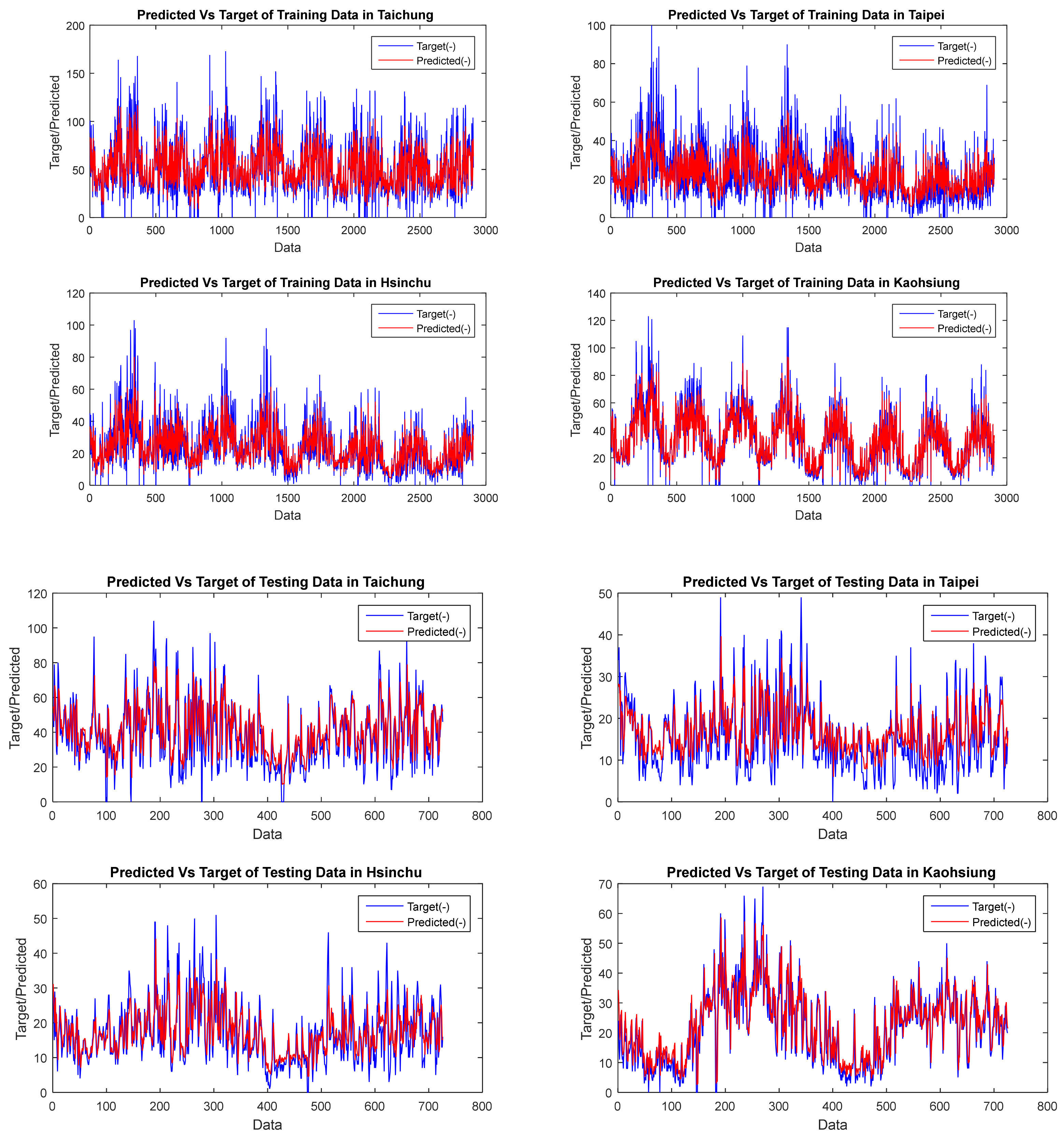
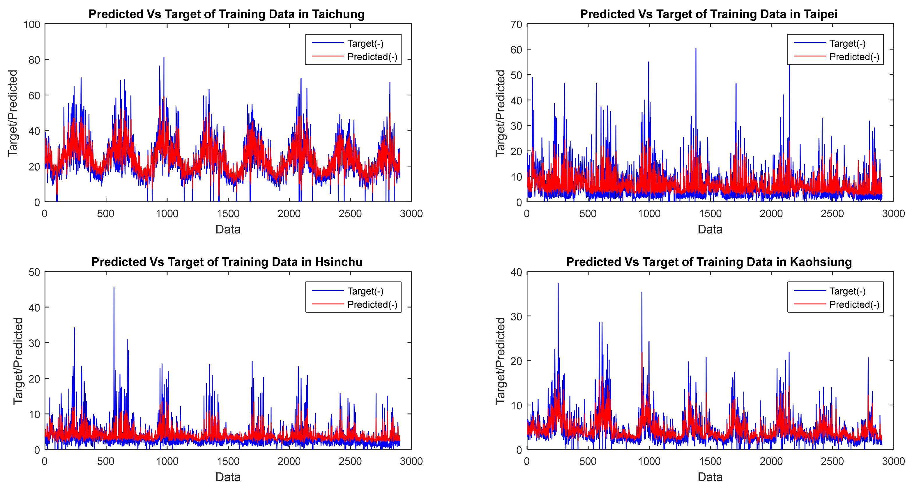
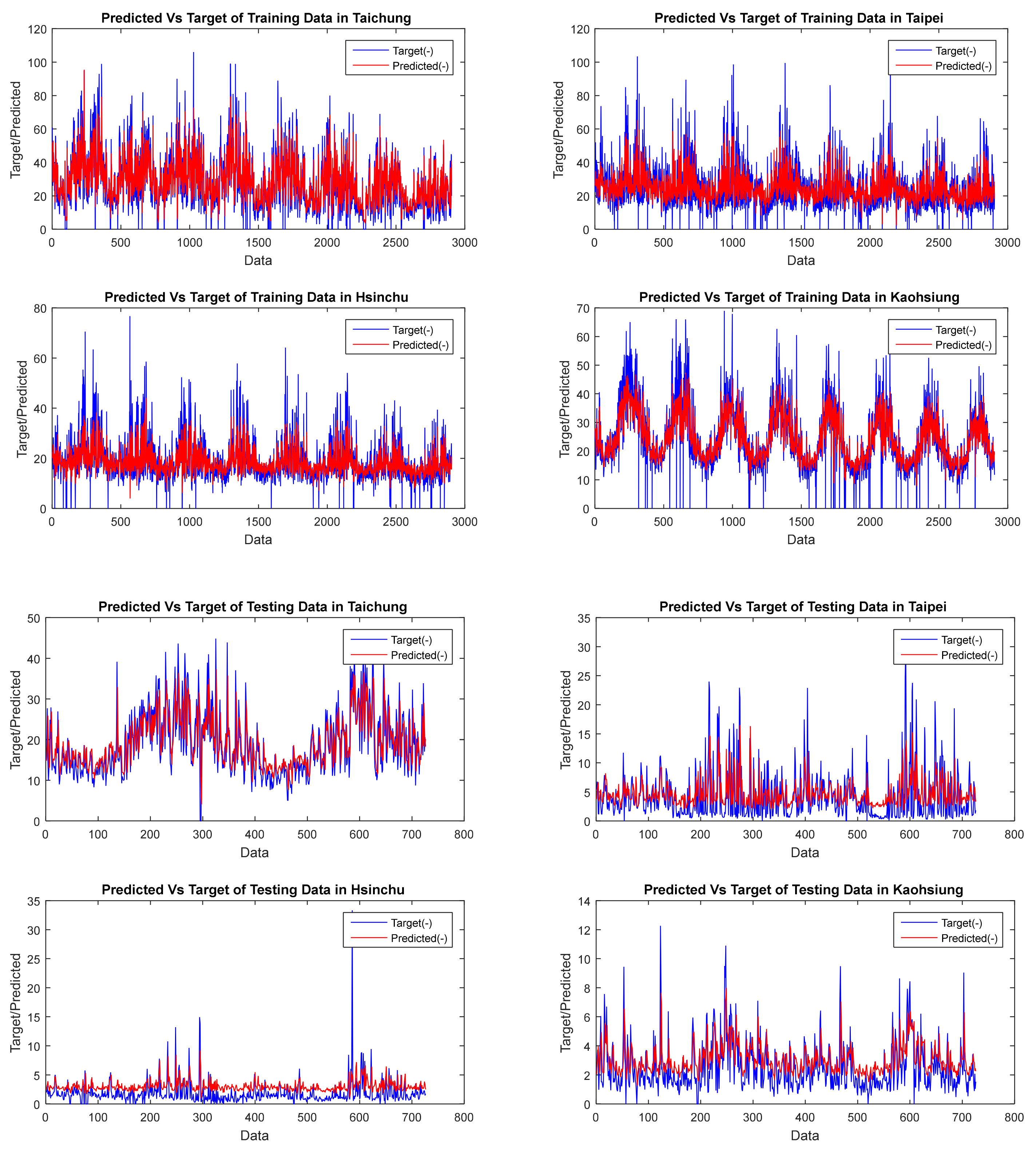
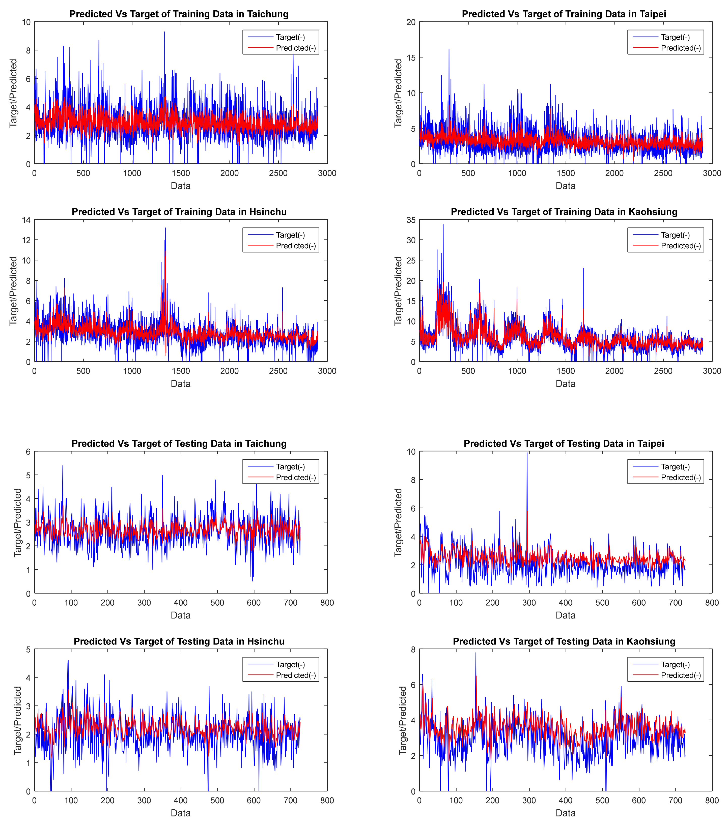
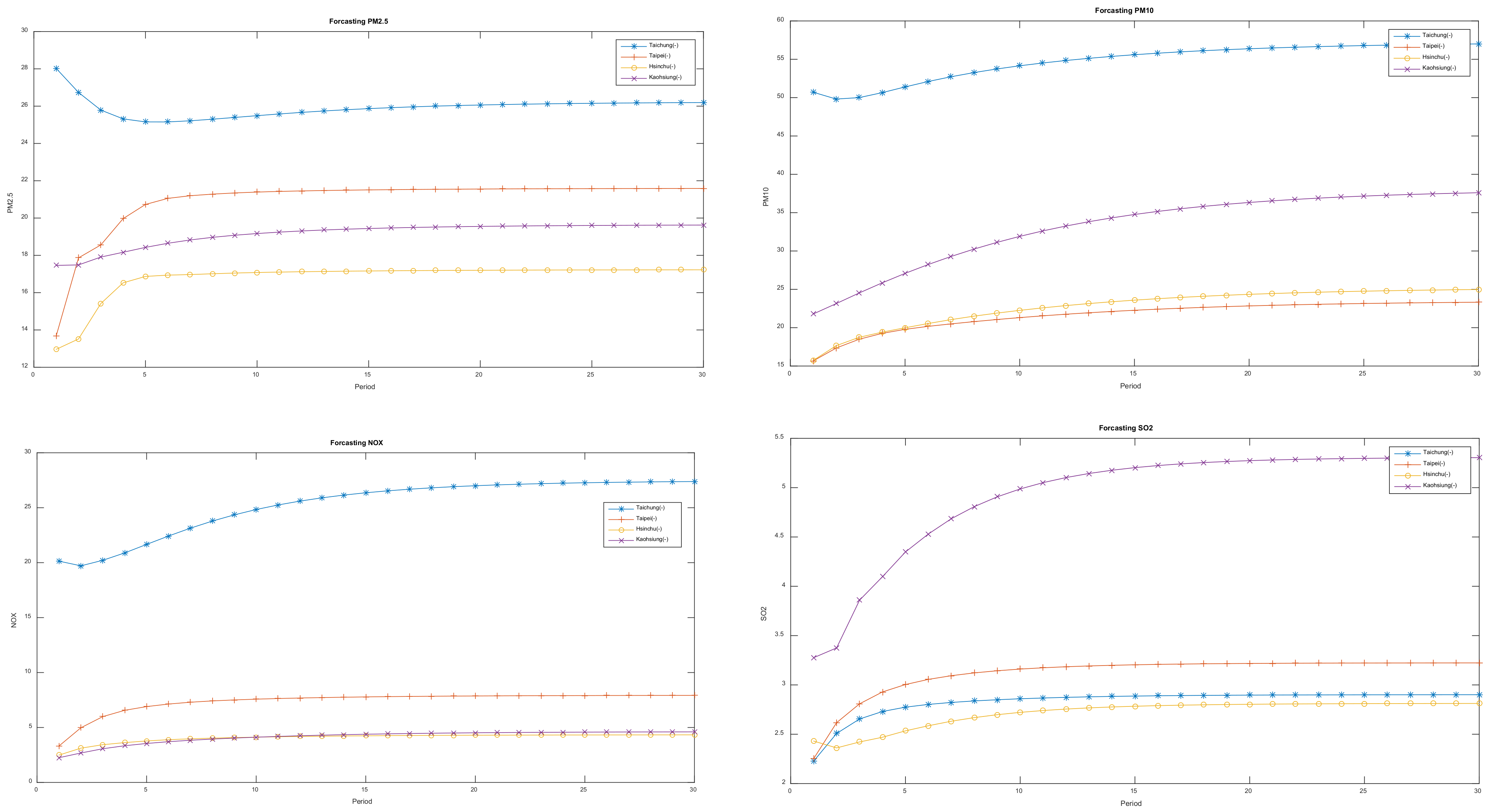
In addition to the time dimension, time series can also have space and time or space-time dimensions. The space-time model is a model that combines elements of time and location dependencies in multivariate time series data, for example, the hourly level of air pollution at several observation points in one area. The generalized space-time autoregressive (GSTAR) model is a model that can overcome the assumption that research locations are heterogeneous; thus, the parameters for each location are different, which is represented in Figure 3, Figure 4, Figure 5 and Figure 6. Based on the best model we forecasted for the next 30 days, it can be seen in Figure 7 that in Taiwan, Taichung city has the most significant values for PM2.5, PM10, NOx, and SO2 values compared to Taipei, Hsinchu, and Kaohsiung. It can be said that the city of Taichung is significantly impacting air pollution; thus, special handling is needed to solve this air pollution problem, especially with penta-helix contributors. Excessive industrial activities can also cause air pollution. In addition, the number of fossil-fueled vehicles contributes to an increase in the amount of carbon dioxide and other toxic gases in the air. Forecasting using GSTAR-CFNN-PSO can be used as a reference for long-term forecasting because it provides a high accuracy value [22,35,40,54,55,56]. In this study, we compared the performance of neural network methods to air pollution. We proposed using two hybrid models that combine VAR and GSTAR with neural network models to forecast pollution. In our proposed model, a time series is considered a nonlinear function of several past observations and random errors. Therefore, VAR and GSTAR models are used to generate the residuals. We first examined the accuracy of these three models using simulated data and then the pollution data. All of our methods yielded almost the same values regardless of leading time. The cascade neural network with PSO was better for the pollution forecast if we consider the training time.
Pollution issues in several countries are specifically related to traffic jams, air and noise pollution, traffic accidents, and delays (increased travel time) [57,58,59,60,61,62,63,64,65,66]. In the late 1980s, developed countries reached a much more advanced stage in transportation planning than they had 20 years earlier. The rapid advancement of knowledge in electronics and computer equipment has enabled the development of several previously unimagined transportation infrastructure concepts. On the other hand, many developing countries are dealing with transportation issues, some of which are already critical. Problems caused by limited existing transportation infrastructure have been added to other issues such as low per capita income, rapid urbanization, limited resources (particularly funds), and the quality and quantity of data related to transportation [4,67,68,69]. It is simple to determine the cause of traffic jams in Taiwan with our bare eyes. Congestion is caused by an increasing uncontrolled number of vehicles, including cars, motorcycles, public transit, and other vehicles, which then spill into traffic, causing this general problem. Furthermore, the number of private cars is increasing. It can be seen that the number of cars on major roads outnumbers other vehicles such as motorcycles, public transportation, and so on.

5. Conclusions

The GSTAR model has limitations, as it cannot model nonlinear time series. This can be overcome by applying a hybrid model to the GSTAR. The hybrid model works by combining linear and nonlinear models to handle linear and nonlinear correlation structures. Each model produces different error values, and it has been discussed that, overall, the GSTAR-cascade-neural-network model provides better accuracy when compared to the VAR model. Therefore, the pollution conditions, including NOx, PM2.5, PM10, and SO2 in the four locations of Taichung, Taipei, Kaohsiung, and Hsinchu, can be generalized for spatial forecasting using the GSTAR-cascade-neural-network with a reasonably high accuracy up to 0.01% (close to zero). Further research also needs to involve subset elements in the GSTAR model to improve forecast accuracy. In addition, it is possible to develop a GSTARX-ANN 1-level hybrid model for space-time data forecasting as a comparison of the GSTARX-ANN 2-level hybrid model for forecasting data containing trend, seasonal, calendar variation, and linear and nonlinear noise series components. In addition, we recommend using other types of architecture on neural networks and deep neural networks. Further research can be conducted with simulation studies for seasonal data only and seasonal and non-seasonal using the GSTAR-GLS and GSTAR-SUR models. Due to rapid urbanization and industrialization over the last decades, Taiwan has faced severe environmental problems, including air pollution. To address the issue of air pollution, the government has undertaken a number of defensive measures. In line with this, spatial-temporal empirical studies of air quality using monitoring data from the last ten years revealed that air quality changed with urban development. The evaluations are used to make future specific recommendations and policy advice [66,70,71,72,73,74]. In many countries, traffic is the leading cause of serious air pollution. Traffic is a serious threat to the environment not only because of the number of cars on the road, but also because of the fuel efficiency. The per-vehicle mileage in Taiwan is excessively high when compared to other metropolitan cities because Taiwan’s transportation policy has emphasized expanding the supply of traffic utilities, such as through road construction, and expanding intersections and parking lots due to low fuel and parking fees.
Many researchers make observations about pollutant gases, such as ozone (O3), nitrogen oxide (NO), nitrogen dioxide (NO2), sulfur dioxide (SO2), and particulate matter, to determine the air quality in an area and control the stability of its air quality. The research process is carried out by forming an air quality model and then creating a control device to prevent or reduce pollutant substances in the air. Due to the high cost of these controllers and the high maintenance costs, it is not possible to place and use as many tools as possible to measure pollutant concentrations. Therefore, the estimation of pollutant concentration is essential in predicting pollutant concentrations in the future and estimating pollutant concentrations in areas that are not included in the radius of a measuring instrument. The next research can use the air pollution model with chemical transport. This model is a linear dynamic model that is then formed into a state-space model and discrete model, which can be performed using VAR. After that, it is processed at the prediction, correction, and simulation stages.
C t ~ 2 C x 2 C t ~ K x 2 C x 2
C is the concentration of the substance in the air and t is time in seconds. However, K x is the proportional constant in units of m 2 second .
We have explained how to perform vector autoregression with a cascade neural network and particle swarm optimization. The disadvantage of VAR models is that they only can capture the relationship between multiple quantities as they change over time. Every region has different uniqueness of climate phenomena and pollution, making the accuracy for forecasting not really robust.

Author Contributions

Conceptualization, R.E.C. and H.Y.; methodology, R.E.C. and H.Y.; software, R.E.C. and H.Y.; validation, R.E.C. and H.Y.; formal analysis, R.E.C.; investigation, R.E.C.; resources, R.E.C.; data curation, R.E.C.; writing—original draft preparation, R.E.C. and H.Y.; writing—review and editing, T.T., R.E.C., H.Y. and B.P.; visualization, R.E.C. and H.Y. All authors have read and agreed to the published version of the manuscript.

Funding

This research is supported by Padjadjaran University (Jatinangor, Jawa Barat, Indonesia). This research is also supported by the Multidisciplinary Digital Publishing Institute under a research grant and by Rezzy Eko Caraka as a guest editor.

Institutional Review Board Statement

Not applicable.

Informed Consent Statement

Not applicable.

Data Availability Statement

A supplementary code to this article can be found online at https://github.com/Rezzy94/cascadenn (accessed on 24 April 2022).

Conflicts of Interest

The authors declare no conflict of interest. The results are appropriately placed in the context of prior and existing research. This paper has been reviewed in three rounds by independent reviewers. It does not affect the position of the corresponding author as a member of the editorial board in the Special Issue “Recent Topics of Climate Vulnerability: Statistics, Machine Learning, and Data Science, from Theory to Application”.

References

  1. Liao, L.; Du, M.; Chen, Z. Air Pollution, Health Care Use and Medical Costs: Evidence from China. Energy Econ. 2021, 95, 105132. [Google Scholar] [CrossRef]
  2. Bakolis, I.; Hammoud, R.; Stewart, R.; Beevers, S.; Dajnak, D.; MacCrimmon, S.; Broadbent, M.; Pritchard, M.; Shiode, N.; Fecht, D.; et al. Mental Health Consequences of Urban Air Pollution: Prospective Population-Based Longitudinal Survey. Soc. Psychiatry Psychiatr. Epidemiol. 2021, 56, 1587–1599. [Google Scholar] [CrossRef] [PubMed]
  3. WHO. Review of Evidence on Health Aspects of Air Pollution—REVIHAAP; WHO: Geneva, Switzerland, 2021. [Google Scholar]
  4. Shi, Y.; Bilal, M.; Ho, H.C.; Omar, A. Urbanization and Regional Air Pollution across South Asian Developing Countries—A Nationwide Land Use Regression for Ambient PM2.5 Assessment in Pakistan. Environ. Pollut. 2020, 266, 115145. [Google Scholar] [CrossRef] [PubMed]
  5. De Gooijer, J.G.; Hyndman, R.J. 25 Years of Time Series Forecasting. Int. J. Forecast. 2006, 22, 443–473. [Google Scholar] [CrossRef] [Green Version]
  6. Makridakis, S.; Hibon, M. The M3-Competition: Results, Conclusions and Implications. Int. J. Forecast. 2000, 16, 451–476. [Google Scholar] [CrossRef]
  7. Makridakis, S.; Spiliotis, E.; Assimakopoulos, V. The M4 Competition: 100,000 Time Series and 61 Forecasting Methods. Int. J. Forecast. 2020, 36, 54–74. [Google Scholar] [CrossRef]
  8. Makridakis, S. A Survey of Time Series. Int. Stat. Rev. 1976, 44, 29. [Google Scholar] [CrossRef]
  9. Caraka, R.E.; Chen, R.C.; Yasin, H.; Lee, Y.; Pardamean, B. Hybrid Vector Autoregression Feedforward Neural Network with Genetic Algorithm Model for Forecasting Space-Time Pollution Data. Indones. J. Sci. Technol. 2021, 6, 243–266. [Google Scholar] [CrossRef]
  10. Suhartono, S. Time Series Forecasting by Using Seasonal Autoregressive Integrated Moving Average: Subset, Multiplicative or Additive Model. J. Math. Stat. 2011, 7, 20–27. [Google Scholar] [CrossRef]
  11. Makridakis, S.; Spiliotis, E.; Assimakopoulos, V. M5 Accuracy Competition: Results, Findings, and Conclusions. Int. J. Forecast. 2022, 38. [Google Scholar] [CrossRef]
  12. Theodorou, E.; Wang, S.; Kang, Y.; Spiliotis, E.; Makridakis, S.; Assimakopoulos, V. Exploring the Representativeness of the M5 Competition Data. Int. J. Forecast. 2021. [Google Scholar] [CrossRef]
  13. Hewamalage, H.; Bergmeir, C.; Bandara, K. Global Models for Time Series Forecasting: A Simulation Study. Pattern Recognit. 2022, 124, 108441. [Google Scholar] [CrossRef]
  14. Li, Y.; Ye, Q.; Liu, A.; Meng, F.; Zhang, W.; Xiong, W.; Wang, P.; Wang, C. Seeking Urbanization Security and Sustainability: Multi-Objective Optimization of Rainwater Harvesting Systems in China. J. Hydrol. 2017, 550, 42–53. [Google Scholar] [CrossRef]
  15. Suhermi, N.; Suhartono; Prastyo, D.D.; Ali, B. Roll Motion Prediction Using a Hybrid Deep Learning and ARIMA Model. Procedia Comput. Sci. 2018, 144, 251–258. [Google Scholar] [CrossRef]
  16. Suhartono; Maghfiroh, B.; Rahayu, S.P. Hybrid VARX-SVR and GSTARX-SVR for Forecasting Spatio-Temporal Data. Int. J. Innov. Technol. Explor. Eng. IJITEE 2019, 8, 212–218. [Google Scholar]
  17. Ruiz-Aguilar, J.J.; Turias, I.J.; Jiménez-Come, M.J. Hybrid Approaches Based on SARIMA and Artificial Neural Networks for Inspection Time Series Forecasting. Transp. Res. Part E Logist. Transp. Rev. 2014, 67, 37–49. [Google Scholar] [CrossRef]
  18. He, K.; Ji, L.; Wu, C.W.D.; Tso, K.F.G. Using SARIMA–CNN–LSTM Approach to Forecast Daily Tourism Demand. J. Hosp. Tour. Manag. 2021, 49, 25–33. [Google Scholar] [CrossRef]
  19. Zhang, J. Investment Risk Model Based on Intelligent Fuzzy Neural Network and VaR. J. Comput. Appl. Math. 2020, 371, 112707. [Google Scholar] [CrossRef]
  20. Soltani, S.; Modarres, R.; Eslamian, S.S. The Use of Time Series Modeling for the Determination of Rainfall Climates of Iran. Int. J. Climatol. 2007, 27, 819–829. [Google Scholar] [CrossRef]
  21. Box, G.E.P.; Jenkins, G.M.; Reinsel, G.C. Time Series Analysis: Forecasting & Control; John Wiley & Sons: Hoboken, NJ, USA, 1994; ISBN 8131716333. [Google Scholar]
  22. Suhartono; Prastyo, D.D.; Kuswanto, H.; Lee, M.H. Comparison between VAR, GSTAR, FFNN-VAR and FFNN-GSTAR Models for Forecasting Oil Production Methods. Mat. Malays. J. Ind. Appl. Math. 2018, 34, 103–111. [Google Scholar]
  23. Bebis, G.; Georgiopoulos, M. Feed-Forward Neural Networks. IEEE Potentials 1994, 13, 27–31. [Google Scholar] [CrossRef]
  24. Huang, S.N.; Tan, K.K.; Lee, T.H.; Giam, T.S. Decentralized Adaptive Control of Nonlinear Systems Using Neural Networks. Proc. IEEE Conf. Decis. Control 2002, 2, 1757–1761. [Google Scholar] [CrossRef]
  25. Bodyanskiy, Y.V.; Tyshchenko, A.K.; Deineko, A.A. An Evolving Radial Basis Neural Network with Adaptive Learning of Its Parameters and Architecture. Autom. Control Comput. Sci. 2015, 49, 255–260. [Google Scholar] [CrossRef]
  26. Glorot, X.; Bengio, Y. Understanding the Difficulty of Training Deep Feedforward Neural Networks. In Proceedings of the Thirteenth International Conference on Artificial Intelligence and Statistics, Setti Ballas, Italy, 13–15 May 2010; Volume 9, pp. 249–256. [Google Scholar]
  27. Recknagel, F. Applications of Machine Learning to Ecological Modelling. Ecol. Model. 2001, 146, 303–310. [Google Scholar] [CrossRef]
  28. Toharudin, T.; Pontoh, R.S.; Caraka, R.E.; Zahroh, S.; Lee, Y.; Chen, R.C. Employing Long Short-Term Memory and Facebook Prophet Model in Air Temperature Forecasting. Commun. Stat. Simul. Comput. 2021, 1–12. [Google Scholar] [CrossRef]
  29. Helmini, S.; Jihan, N.; Jayasinghe, M.; Perera, S. Sales Forecasting Using Multivariate Long Short Term Memory Networks. PeerJ Prepr. 2019, 7, e27712v1. [Google Scholar] [CrossRef]
  30. Yamak, P.T.; Yujian, L.; Gadosey, P.K. A Comparison between ARIMA, LSTM, and GRU for Time Series Forecasting. In Proceedings of the 2nd International Conference on Algorithms, Computing and Artificial Intelligence, Sanya, China, 20–22 December 2019; pp. 49–55. [Google Scholar]
  31. Li, D. Human Skeleton Detection and Extraction in Dance Video Based on PSO-Enabled LSTM Neural Network. Comput. Intell. Neurosci. 2021, 2021, 2545151. [Google Scholar] [CrossRef]
  32. AgaAzizi, S.; Rasekh, M.; Abbaspour-Gilandeh, Y.; Kianmehr, M.H. Identification of Impurity in Wheat Mass Based on Video Processing Using Artificial Neural Network and PSO Algorithm. J. Food Processing Preserv. 2021, 45, e15067. [Google Scholar] [CrossRef]
  33. Shafiei Chafi, Z.; Afrakhte, H. Short-Term Load Forecasting Using Neural Network and Particle Swarm Optimization (PSO) Algorithm. Math. Probl. Eng. 2021, 2021, 5598267. [Google Scholar] [CrossRef]
  34. Quarto, M.; D’urso, G.; Giardini, C.; Maccarini, G.; Carminati, M. A Comparison between Finite Element Model (Fem) Simulation and an Integrated Artificial Neural Network (Ann)-Particle Swarm Optimization (Pso) Approach to Forecast Performances of Micro Electro Discharge Machining (Micro-Edm) Drilling. Micromachines 2021, 12, 667. [Google Scholar] [CrossRef]
  35. Suhartono; Wahyuningrum, S.R.; Setiawan; Akbar, M.S. GSTARX-GLS Model for Spatio-Temporal Data Forecasting. Malays. J. Math. Sci. 2016, 10, 91–103. [Google Scholar]
  36. Astutik, S.; Iriawan, N.; Nair, G.; Suhartono. Sutikno Bayesian State Space Modeling for Spatio-Temporal Rainfall Disaggregation. Int. J. Appl. Math. Stat. 2013, 37, 26–37. [Google Scholar]
  37. Suhartono, A. Comparative Study of Forecasting Models for Trend and Seasonal Time Series: Does Complex Model Always Yield Better Forecast Than Simple Model. J. Tek. Ind. 2005, 7, 22–30. [Google Scholar] [CrossRef]
  38. Delforge, D.; Watlet, A.; Kaufmann, O.; Van Camp, M.; Vanclooster, M. Time-Series Clustering Approaches for Subsurface Zonation and Hydrofacies Detection Using a Real Time-Lapse Electrical Resistivity Dataset. J. Appl. Geophys. 2021, 184, 104203. [Google Scholar] [CrossRef]
  39. Suhartono, S.; Subanar, S. Some Comments on the Theorem Providing Stationarity Condition for Gstar Models in the Paper by Borovkova Et Al. J. Indones. Math. Soc. 2007, 13, 115–121. [Google Scholar] [CrossRef] [Green Version]
  40. Ruchjana, B.N.; Borovkova, S.A.; Lopuhaa, H.P. Least Squares Estimation of Generalized Space Time AutoRegressive (GSTAR) Model and Its Properties. In AIP Conference Proceedings; American Institute of Physics: College Park, MD, USA, 2012; Volume 1450, pp. 61–64. [Google Scholar]
  41. Wei, W.W.S.; Hamilton, J.D. Time Series Analysis; Prentice Hall: Hoboken, NJ, USA, 1994; pp. 837–900. [Google Scholar]
  42. Kennedy, J.; Eberhart, R. Particle Swarm Optimization. In 1995 IEEE International Conference on Neural Networks Proceedings; IEEE: Piscataway, NJ, USA, 1995; Volume 4, pp. 1942–1948. [Google Scholar] [CrossRef]
  43. Caraka, R.E.; Chen, R.C.; Yasin, H.; Pardamean, B.; Toharudin, T.; Wu, S.H. Prediction of Status Particulate Matter 2.5 Using State Markov Chain Stochastic Process and HYBRID VAR-NN-PSO. IEEE Access 2019, 7, 161654–161665. [Google Scholar] [CrossRef]
  44. Rahman, C.M.; Rashid, T.A. Dragonfly Algorithm and Its Applications in Applied Science Survey. Comput. Intell. Neurosci. 2019, 2019, 9293617. [Google Scholar] [CrossRef]
  45. Khursheed, M.U.N.; Nadeem, M.F.; Khalil, A.; Sajjad, I.A.; Raza, A.; Iqbal, M.Q.; Bo, R.; Rehman, W.U. Review of Flower Pollination Algorithm: Applications and Variants. In Proceedings of the 2020 International Conference on Engineering and Emerging Technologies, ICEET 2020, Lahore, Pakistan, 22–23 February 2020; Institute of Electrical and Electronics Engineers Inc.: Piscataway, NJ, USA, 2020. [Google Scholar]
  46. Karaboga, D.; Basturk, B. A Powerful and Efficient Algorithm for Numerical Function Optimization: Artificial Bee Colony (ABC) Algorithm. J. Glob. Optim. 2007, 39, 459–471. [Google Scholar] [CrossRef]
  47. Setiawan, S.; Prastuti, M. S-GSTAR-SUR Model for Seasonal Spatio Temporal Data Forecasting. Malays. J. Math. Sci. 2016, 10, 53–65. [Google Scholar]
  48. Parker, P.; Swindlehurst, A. Space-Time Autoregressive Filtering for Matched Subspace STAP. IEEE Trans. Aerosp. Electron. Syst. 2003, 39, 510–520. [Google Scholar] [CrossRef]
  49. Storvik, G.; Frigessi, A.; Hirst, D. Stationary Space-Time Gaussian Fields and Their Time Autoregressive Representation. Stat. Modeling 2002, 2, 139–161. [Google Scholar] [CrossRef] [Green Version]
  50. Cheng, T.; Wang, J.; Haworth, J.; Heydecker, B.; Chow, A. A Dynamic Spatial Weight Matrix and Localized Space-Time Autoregressive Integrated Moving Average for Network Modeling. Geogr. Anal. 2014, 46, 75–97. [Google Scholar] [CrossRef]
  51. Prastyo, D.D.; Nabila, F.S.; Suhartono; Lee, M.H.; Suhermi, N.; Fam, S.F. VAR and GSTAR-Based Feature Selection in Support Vector Regression for Multivariate Spatio-Temporal Forecasting. In Proceedings of the Communications in Computer and Information Science, Dresden, Germany, 10–11 October 2019; pp. 46–57. [Google Scholar]
  52. Abdullah, A.S.; Matoha, S.; Lubis, D.A.; Falah, A.N.; Jaya, I.G.N.M.; Hermawan, E.; Ruchjana, B.N. Implementation of Generalized Space Time Autoregressive (GSTAR)-Kriging Model for Predicting Rainfall Data at Unobserved Locations in West Java. Appl. Math. Inf. Sci. 2018, 12, 607–615. [Google Scholar] [CrossRef]
  53. Caraka, R.E.; Yasin, H.; Chen, R.C.; Goldameir, N.E.; Supatmanto, B.D.; Toharudin, T.; Basyuni, M.; Gio, P.U. Evolving Hybrid Cascade Neural Network Genetic Algorithm Space-Time Forecasting. Symmetry 2021, 13, 1158. [Google Scholar] [CrossRef]
  54. Bonar, H.; Ruchjana, B.N.; Darmawan, G. Development of Generalized Space Time Autoregressive Integrated with ARCH Error (GSTARI—ARCH) Model Based on Consumer Price Index Phenomenon at Several Cities in North Sumatera Province. In AIP Conference Proceedings; AIP Publishing LLC: Melville, NY, USA, 2017. [Google Scholar]
  55. Borovkova, S.; Lopuhaä, H.P.; Ruchjana, B.N. Consistency and Asymptotic Normality of Least Squares Estimators in Generalized STAR Models. Stat. Neerl. 2008, 62, 482–508. [Google Scholar] [CrossRef]
  56. Yundari, Y.; Huda, N.M.; Pasaribu, U.S.; Mukhaiyar, U.; Sari, K.N. Stationary process in GSTAR (1;1) through kernel function approach. In AIP Conference Proceedings; AIP Publishing LLC: Melville, NY, USA, 2020; Volume 2268, p. 020010. [Google Scholar] [CrossRef]
  57. Zhang, J.J.; Wei, Y.; Fang, Z. Ozone Pollution: A Major Health Hazard Worldwide. Front. Immunol. 2019, 10, 2518. [Google Scholar] [CrossRef] [Green Version]
  58. Riojas-Rodríguez, H.; Romieu, I.; Hernández-Ávila, M. Air Pollution. In Occupational and Environmental Health; Oxford University Press: Oxford, UK, 2017; ISBN 9780190662677. [Google Scholar]
  59. Deryugina, T.; Heutel, G.; Miller, N.H.; Molitor, D.; Reif, J. The Mortality and Medical Costs of Air Pollution: Evidence from Changes in Wind Direction. Am. Econ. Rev. 2019, 109, 4178–4219. [Google Scholar] [CrossRef]
  60. Akimoto, H. Global Air Quality and Pollution. Science 2003, 302, 1716–1719. [Google Scholar] [CrossRef] [Green Version]
  61. Wang, H.; Zhang, H.; Cai, G. An Application of Phytoremediation to River Pollution Remediation. Procedia Environ. Sci. 2011, 10, 1904–1907. [Google Scholar] [CrossRef] [Green Version]
  62. Masseran, N.; Safari, M.A.M. Modeling the Transition Behaviors of PM 10 Pollution Index. Environ. Monit. Assess. 2020, 192, 1–15. [Google Scholar] [CrossRef]
  63. Masseran, N.; Mohd Safari, M.A. Intensity–Duration–Frequency Approach for Risk Assessment of Air Pollution Events. J. Environ. Manag. 2020, 264, 110429. [Google Scholar] [CrossRef] [PubMed]
  64. AL-Dhurafi, N.A.; Masseran, N.; Zamzuri, Z.H. Hierarchical-Generalized Pareto Model for Estimation of Unhealthy Air Pollution Index. Environ. Modeling Assess. 2020, 25, 555–564. [Google Scholar] [CrossRef]
  65. Paoletti, E.; de Marco, A.; Pompei, E. Five-Year Volume Growth of European Beech Does Not Respond to Ozone Pollution in Italy. Environ. Sci. Pollut. Res. 2017, 25, 8233–8239. [Google Scholar] [CrossRef] [PubMed]
  66. Caraka, R.E.; Yusra, Y.; Toharudin, T.; Chen, R.; Basyuni, M. Did Noise Pollution Really Improve during COVID-19? Evidence from Taiwan. Sustainability 2021, 13, 5946. [Google Scholar] [CrossRef]
  67. Tsai, F.; Tu, J.Y.; Hsu, S.C.; Chen, W.N. Case Study of the Asian Dust and Pollutant Event in Spring 2006: Source, Transport, and Contribution to Taiwan. Sci. Total Environ. 2014, 478, 163–174. [Google Scholar] [CrossRef]
  68. De Vos, J. Transportation Research Interdisciplinary Perspectives the Effect of COVID-19 and Subsequent Social Distancing on Travel Behavior. Transp. Res. Interdiscip. Perspect. 2020, 5, 100121. [Google Scholar] [CrossRef]
  69. Wei, G.; Zhang, Z.; Ouyang, X.; Shen, Y.; Jiang, S.; Liu, B.; He, B.J. Delineating the Spatial-Temporal Variation of Air Pollution with Urbanization in the Belt and Road Initiative Area. Environ. Impact Assess. Rev. 2021, 91, 106646. [Google Scholar] [CrossRef]
  70. Gayialis, S.P.; Kechagias, E.P.; Konstantakopoulos, G.D. A City Logistics System for Freight Transportation: Integrating Information Technology and Operational Research. Oper. Res. 2022, 1–30. [Google Scholar] [CrossRef]
  71. Peng, J.; Parnell, J.; Kessissoglou, N. Spatially Differentiated Profiles for Road Traffic Noise Pollution across a State Road Network. Appl. Acoust. 2021, 172, 107641. [Google Scholar] [CrossRef]
  72. Hong, W.C. Traffic Flow Forecasting by Seasonal SVR with Chaotic Simulated Annealing Algorithm. Neurocomputing 2011, 74, 2096–2107. [Google Scholar] [CrossRef]
  73. Li, M.W.; Hong, W.C.; Kang, H.G. Urban Traffic Flow Forecasting Using Gauss-SVR with Cat Mapping, Cloud Model and PSO Hybrid Algorithm. Neurocomputing 2013, 99, 230–240. [Google Scholar] [CrossRef]
  74. Kechagias, E.P.; Gayialis, S.P.; Konstantakopoulos, G.D.; Papadopoulos, G.A. Traffic Flow Forecasting for City Logistics: A Literature Review and Evaluation. Int. J. Decis. Support Syst. 2019, 4, 159–176. [Google Scholar] [CrossRef]
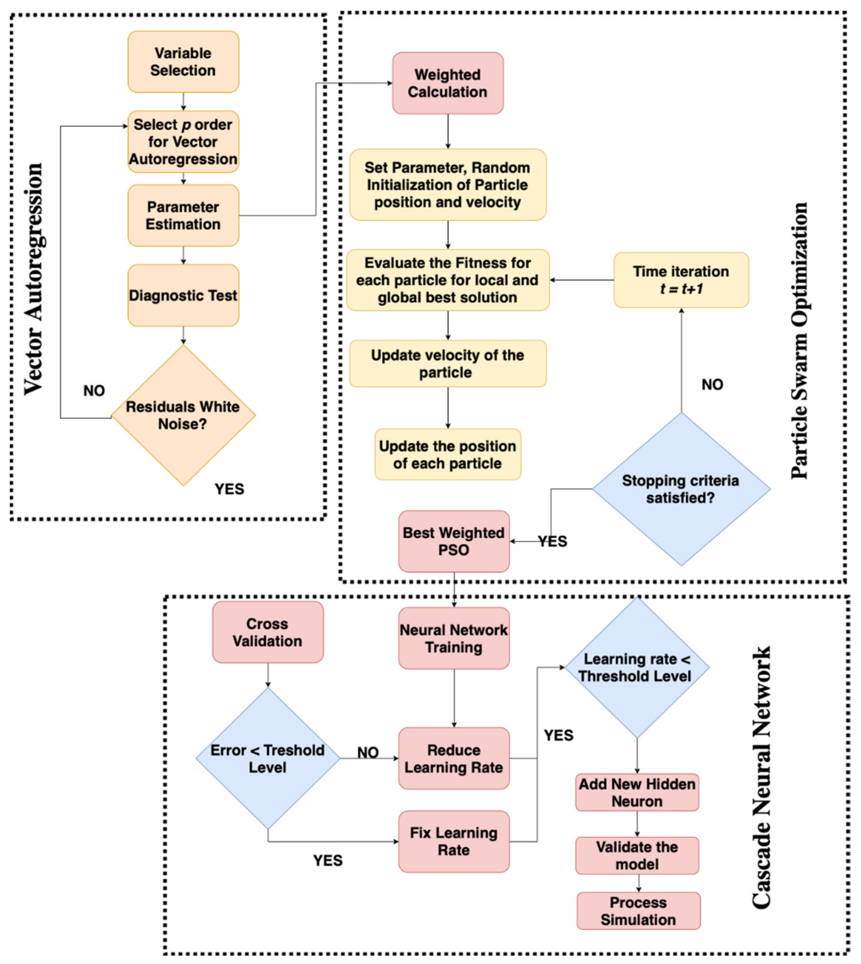
Figure 1. Flowchart VAR-CASCADE NN PSO.
Atmosphere 13 00875 g001
Figure 2. Space-time cascade neural network with particle swarm optimization.
Atmosphere 13 00875 g002
Figure 3. PM10 GSTAR(1) CFNN PSO.
Atmosphere 13 00875 g003
Figure 4. NOx GSTAR(2) CFNN PSO.
Atmosphere 13 00875 g004aAtmosphere 13 00875 g004b
Figure 5. PM2.5 GSTAR(2) CFNN PSO.
Atmosphere 13 00875 g005
Figure 6. SO2 GSTAR(2) CFNN PSO.
Atmosphere 13 00875 g006
Figure 7. GSTAR(2) CFNN PSO forecasting.
Atmosphere 13 00875 g007
Table 1. Model Comparison based on Pollution.
GSTAR CFNNDatasetFVALOBJTrainingTestingAverage Elapsed Time (Seconds)
RMSEMAESMAPERMSEMAESMAPERMSEMAESMAPE
GSTAR (1)NOX0.74700.74705.26603.26220.00494.71432.42820.02684.99022.84520.0159229.0739
PM2.51.15801.15809.28316.50540.00416.79554.99210.02058.03935.74880.012391.236504
PM100.7355710.735613.09069.11460.00389.29946.58050.01611.19507.84760.0099 *90.51314
SO22.6432.6431.54091.05920.00570.90350.68930.02651.22220.87430.016195.544592
GSTAR (2)NOX0.7158550.71595.2033.27470.0053.73582.49010.02394.46942.88240.0145 *106.778741
PM2.52.027282.02739.22376.43610.00426.78474.95620.01998.00425.69620.0121 *120.178632
PM102.41872.418712.94898.98960.00369.13516.42550.016711.04207.70760.0102196.033143
SO27.793967.7941.51721.04650.00560.88580.67260.02571.20150.85960.0157 *206.967525
VAR (1)NOX3.201163.20125.18473.242613.58343.73782.402812.41584.46132.822712.999683.651723
PM2.55.9999569.21646.44737.58026.83115.02476.87078.02385.73607.225583.842196
PM103.318373.318412.91788.97787.239.27316.57618.492411.09557.77707.861284.947817
SO22.655042.6551.53491.05066.82110.91850.70076.49131.22670.87576.656275.589595
VAR (2)NOX7.505727.50575.04663.118312.02343.67442.325411.87134.36052.721911.947482.196178
PM2.55.315125.31519.14316.38547.86896.7775.03067.26657.96015.70807.5677269.645339
PM103.722733.722712.72138.75796.92379.00496.30917.956910.86317.53357.4403105.356041
SO25.475675.47571.4931.0276.79560.90680.68237.15531.19990.85476.9755161.550041
* Best model.
Publisher’s Note: MDPI stays neutral with regard to jurisdictional claims in published maps and institutional affiliations.