
A Deep Learning Approach for Meter-Scale Air Quality Estimation in Urban Environments Using Very High-Spatial-Resolution Satellite Imagery


 ,
,  , ,
, ,  ,
,
Abstract
:1. Introduction
2. Data and Methods
2.1. Data
- Satellite Imagery
- LUR data
- Ground monitoring data
2.2. Methodology
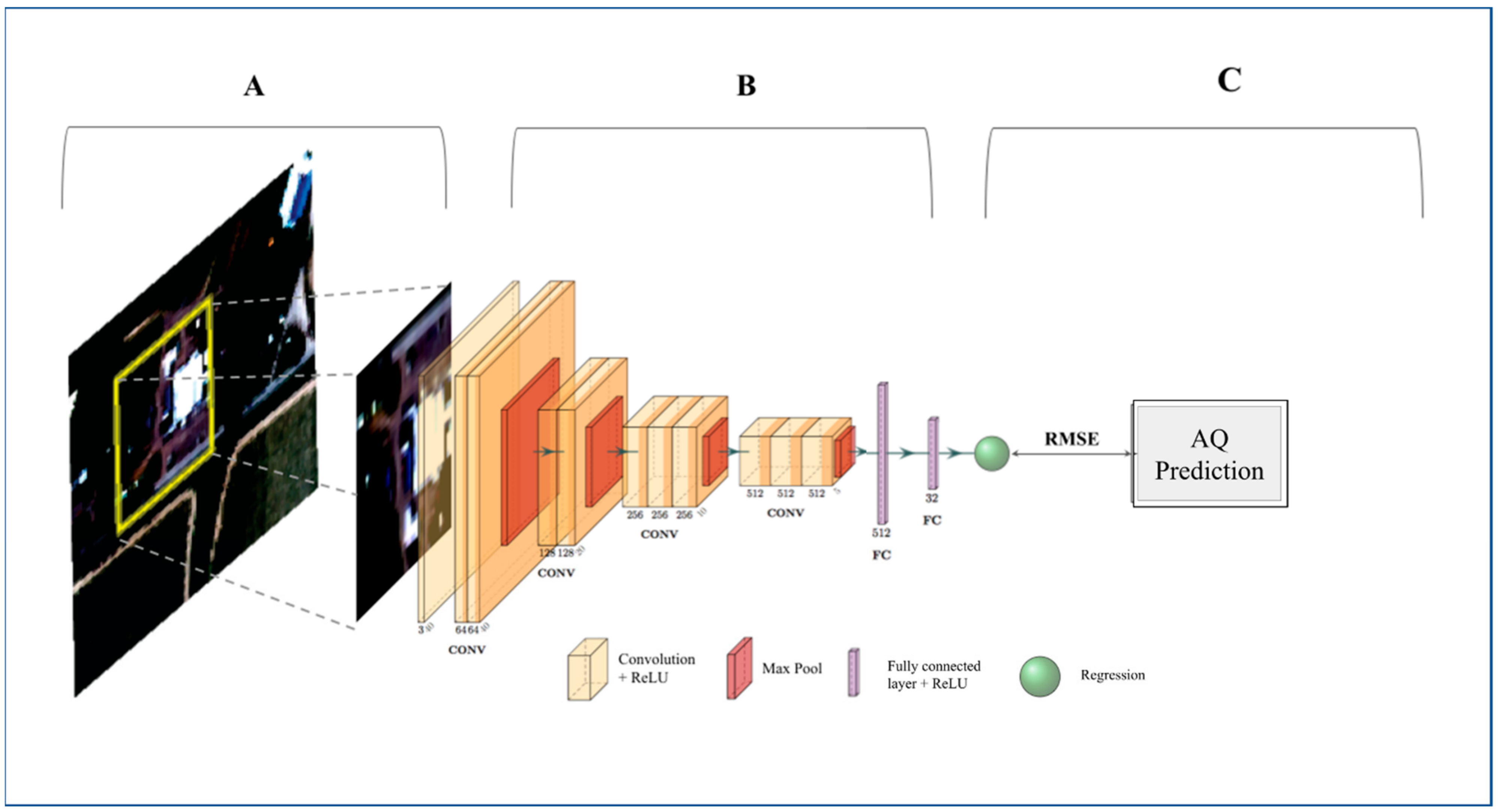
- Model Architecture
- Data Preparation
- Validation
3. Results
- Air Quality Data
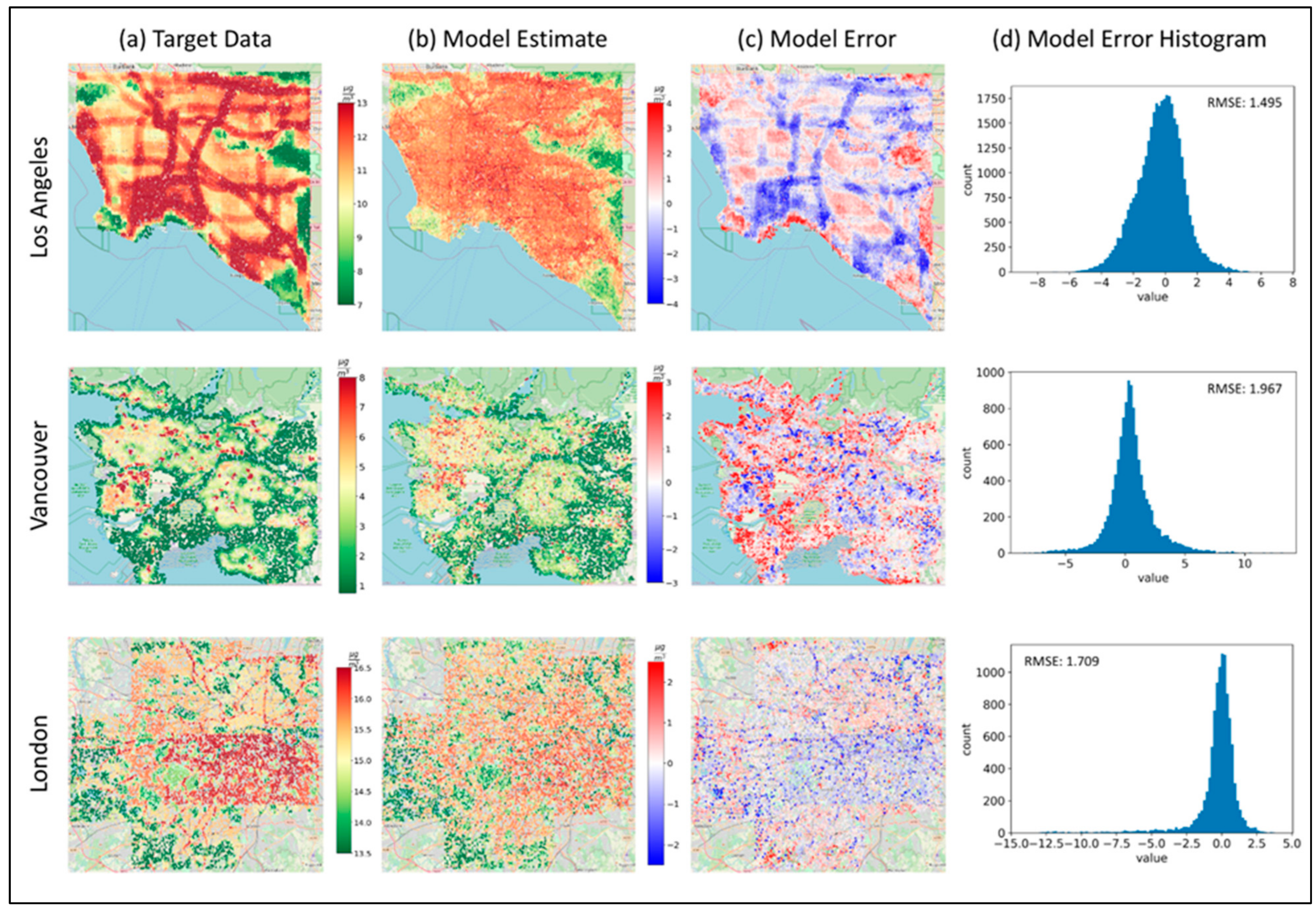
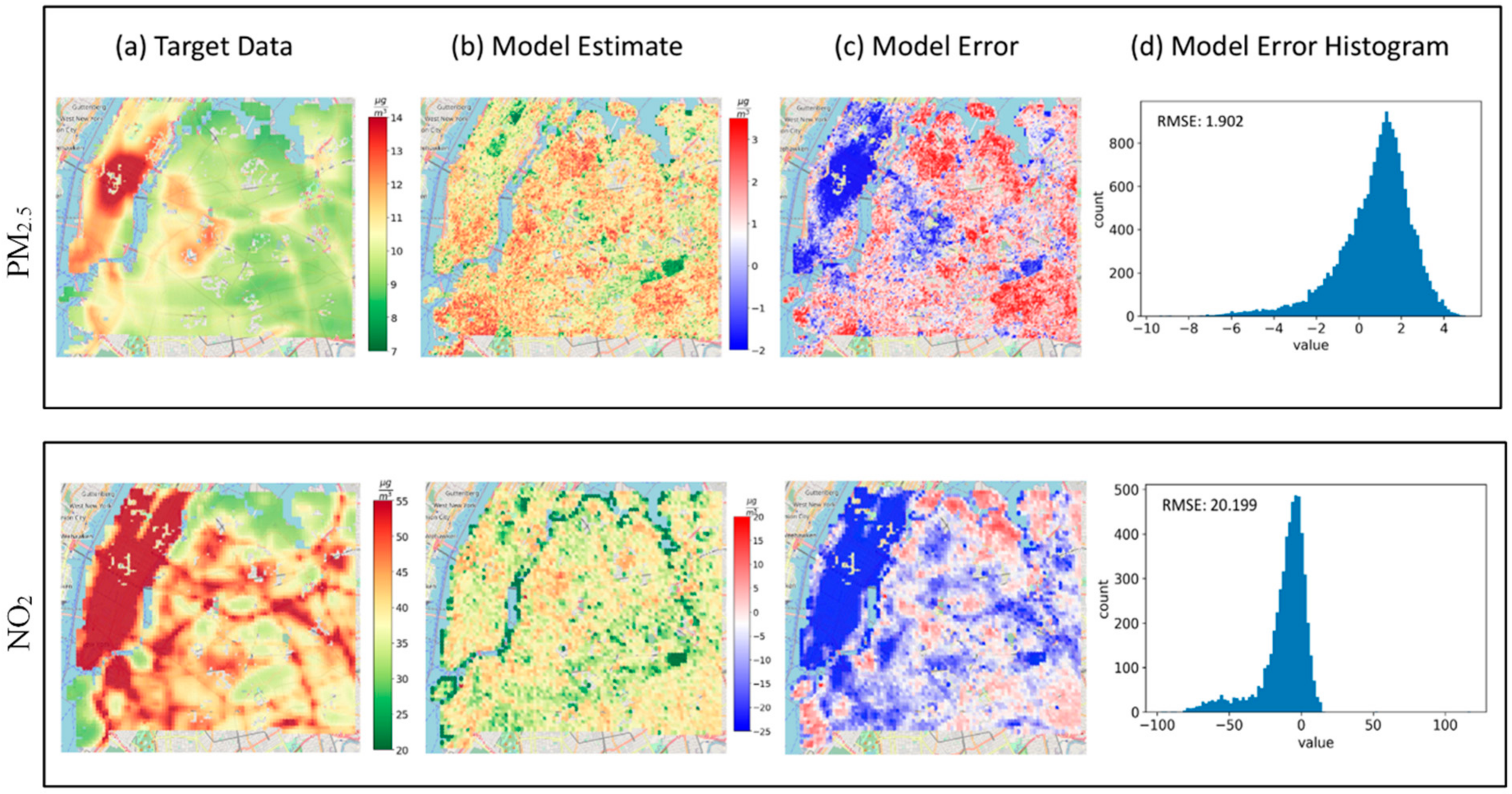
- Estimating PM2.5 Concentrations
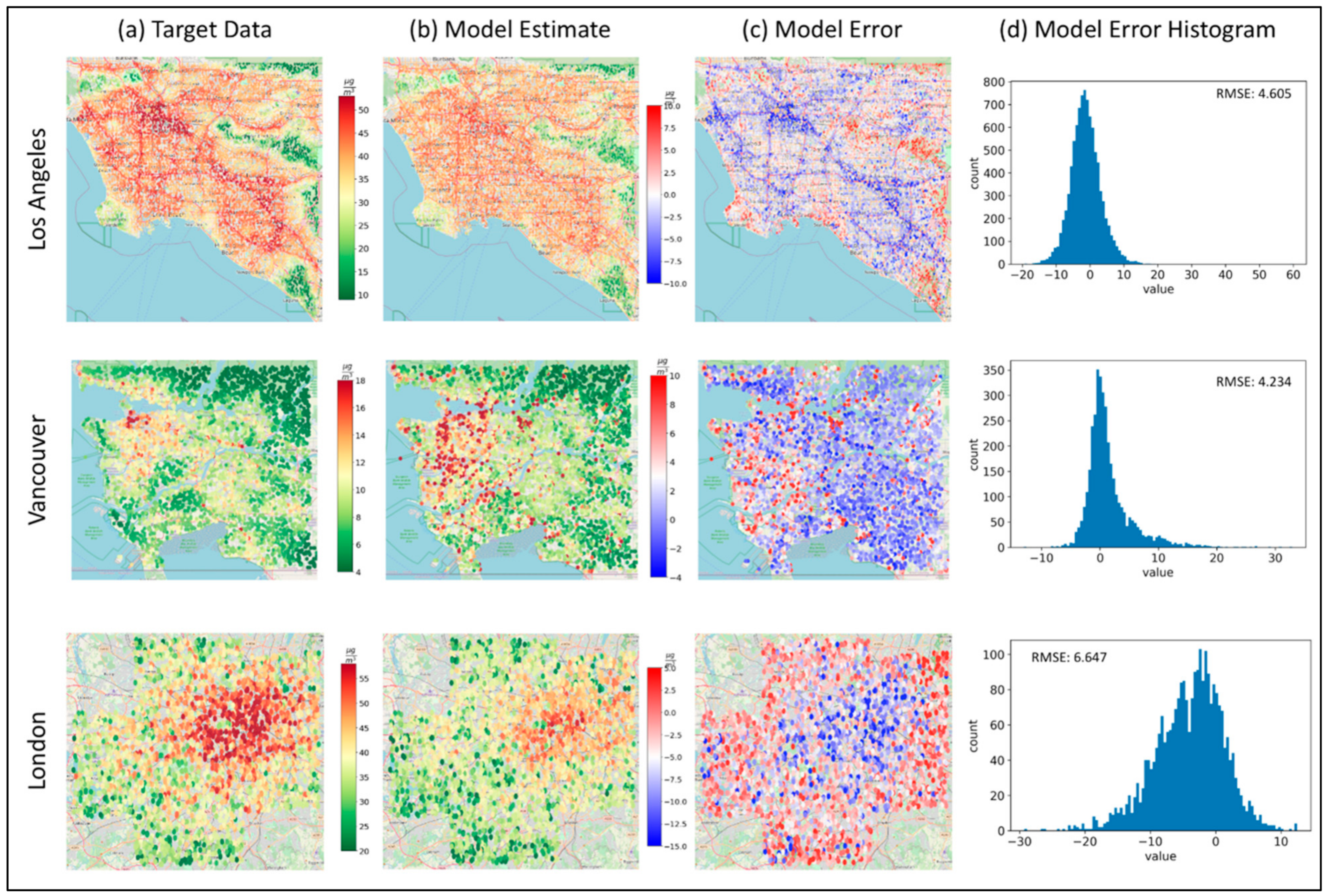
- Estimating NO2 Concentrations
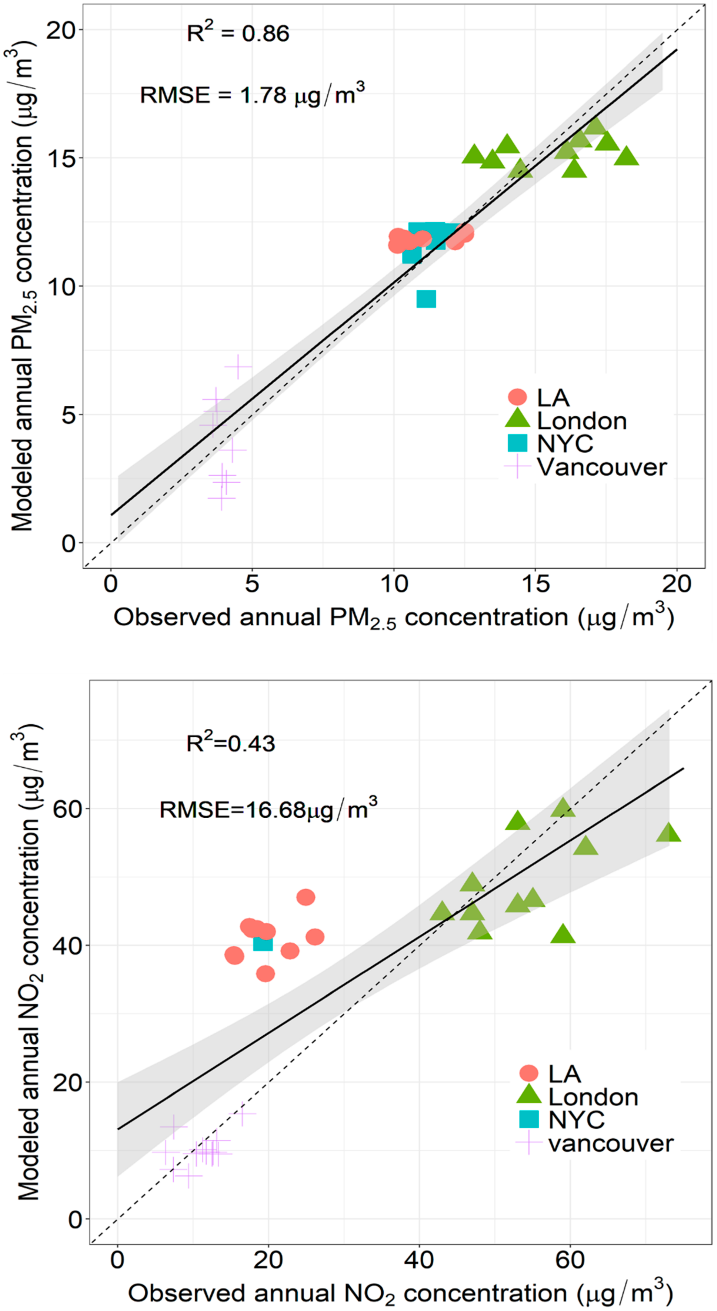
- Validation
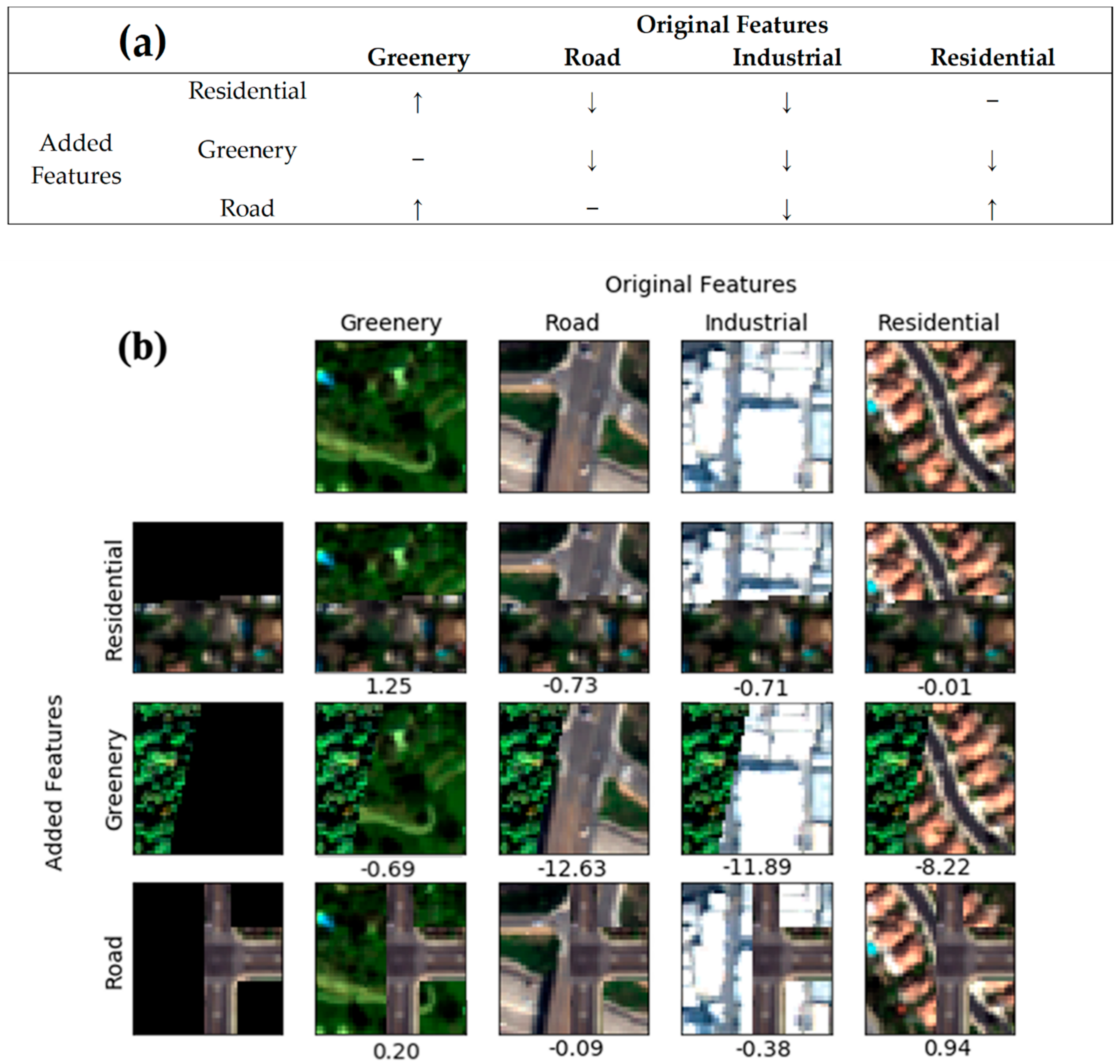
- Model Interpretability
4. Discussion
Supplementary Materials
Author Contributions
Funding
Institutional Review Board Statement
Data Availability Statement
Acknowledgments
Conflicts of Interest
References
- Pope, C.A.; Lefler, J.S.; Ezzati, M.; Higbee, J.D.; Marshall, J.D.; Kim, S.-Y.; Bechle, M.; Gilliat, K.S.; Vernon, S.E.; Robinson, A.L.; et al. Mortality risk and fine particulate air pollution in a large, representative cohort of U.S. adults. Environ. Health Perspect. 2019, 127, 77007. [Google Scholar] [CrossRef] [PubMed]
- Brauer, M. Air quality and health: Looking forward. Air Qual. Clim. Chang. 2017, 51, 23–26. [Google Scholar]
- HEI. State of Global Air Special Report. Health Effects Institute. 2019. Available online: http://www.stateofglobalair.org/sites/default/files/soga_2019_report.pdf (accessed on 1 March 2022).
- Wang, Y.; Bechle, M.J.; Kim, S.-Y.; Adams, P.J.; Pandis, S.N.; Pope, C.A.; Robinson, A.L.; Sheppard, L.; Szpiro, A.A.; Marshall, J.D. Spatial decomposition analysis of NO2 and PM2.5 air pollution in the United States. Atmos. Environ. 2020, 241, 117470. [Google Scholar] [CrossRef]
- Kotchenruther, R.A. Source apportionment of PM2.5 at multiple Northwest U.S. sites: Assessing regional winter wood smoke impacts from residential wood combustion. Atmos. Environ. 2016, 142, 210–219. [Google Scholar] [CrossRef]
- Nguyen, C.; Soulhac, L.; Salizzoni, P. Source apportionment and data assimilation in urban air quality modelling for NO2: The lyon case study. Atmosphere 2018, 9, 8. [Google Scholar] [CrossRef] [Green Version]
- Karagulian, F.; Belis, C.A.; Dora, C.F.C.; Prüss-Ustün, A.M.; Bonjour, S.; Adair-Rohani, H.; Amann, M. Contributions to cities’ ambient particulate matter (PM): A systematic review of local source contributions at global level. Atmos. Environ. 2015, 120, 475–483. [Google Scholar] [CrossRef]
- Isakov, V.; Arunachalam, S.; Baldauf, R.; Breen, M.; Deshmukh, P.; Hawkins, A.; Kimbrough, S.; Krabbe, S.; Naess, B.; Serre, M.; et al. Combining Dispersion Modeling and Monitoring Data for Community-Scale Air Quality Characterization. Atmosphere 2019, 10, 610. [Google Scholar] [CrossRef] [Green Version]
- Van Zoest, V.; Osei, F.B.; Hoek, G.; Stein, A. Spatio-temporal regression kriging for modelling urban NO2 concentrations. Int. J. Geogr. Inf. Sci. 2020, 34, 851–865. [Google Scholar] [CrossRef] [Green Version]
- Jin, L.; Berman, J.D.; Warren, J.L.; Levy, J.I.; Thurston, G.; Zhang, Y.; Xu, X.; Wang, S.; Zhang, Y.; Bell, M.L. A land use regression model of nitrogen dioxide and fine particulate matter in a complex urban core in Lanzhou, China. Environ. Res. 2019, 177, 108597. [Google Scholar] [CrossRef]
- De Hoogh, K.; Gulliver, J.; Donkelaar, A.; van Martin, R.V.; Marshall, J.D.; Bechle, M.J.; Cesaroni, G.; Pradas, M.C.; Dedele, A.; Eeftens, M.; et al. Development of West-European PM2.5 and NO2 land use regression models incorporating satellite-derived and chemical transport modelling data. Environ. Res. 2016, 151, 1–10. [Google Scholar] [CrossRef] [Green Version]
- Bertazzon, S.; Johnson, M.; Eccles, K.; Kaplan, G.G. Accounting for spatial effects in land use regression for urban air pollution modeling. Spat. Spatiotemporal. Epidemiol. 2015, 14–15, 9–21. [Google Scholar] [CrossRef] [PubMed] [Green Version]
- Beelen, R.; Hoek, G.; Vienneau, D.; Eeftens, M.; Dimakopoulou, K.; Pedeli, X.; Tsai, M.-Y.; Künzli, N.; Schikowski, T.; Marcon, A.; et al. Development of NO2 and NOx land use regression models for estimating air pollution exposure in 36 study areas in Europe—The ESCAPE project. Atmos. Environ. 2013, 72, 10–23. [Google Scholar] [CrossRef]
- Ross, Z.; Jerrett, M.; Ito, K.; Tempalski, B.; Thurston, G. A land use regression for predicting fine particulate matter concentrations in the New York City region. Atmos. Environ. 2007, 41, 2255–2269. [Google Scholar] [CrossRef]
- Van Donkelaar, A.; Martin, R.V.; Brauer, M.; Hsu, N.C.; Kahn, R.A.; Levy, R.C.; Lyapustin, A.; Sayer, A.M.; Winker, D.M. Global Estimates of Fine Particulate Matter using a Combined Geophysical-Statistical Method with Information from Satellites, Models, and Monitors. Environ. Sci. Technol. 2016, 50, 3762–3772. [Google Scholar] [CrossRef] [PubMed]
- Kloog, I.; Sorek-Hamer, M.; Lyapustin, A.; Coull, B.; Wang, Y.; Just, A.C.; Schwartz, J.; Broday, D.M. Estimating daily PM2.5 and PM10 across the complex geo-climate region of Israel using MAIAC satellite-based AOD data. Atmos. Environ. 2015, 122, 409–416. [Google Scholar] [CrossRef] [Green Version]
- Engel-Cox, J.A.; Holloman, C.H.; Coutant, B.W.; Hoff, R.M. Qualitative and quantitative evaluation of MODIS satellite sensor data for regional and urban scale air quality. Atmos. Environ. 2004, 38, 2495–2509. [Google Scholar] [CrossRef]
- Hammer, M.S.; van Donkelaar, A.; Li, C.; Lyapustin, A.; Sayer, A.M.; Hsu, N.C.; Levy, R.C.; Garay, M.J.; Kalashnikova, O.V.; Kahn, R.A.; et al. Global Estimates and Long-Term Trends of Fine Particulate Matter Concentrations (1998–2018). Environ. Sci. Technol. 2020, 54, 7879–7890. [Google Scholar] [CrossRef]
- Sorek-Hamer, M.; Franklin, M.; Chau, K.; Garay, M.; Kalashnikova, O. Spatiotemporal Characteristics of the Association between AOD and PM over the California Central Valley. Remote Sens. 2020, 12, 685. [Google Scholar] [CrossRef] [Green Version]
- Van Donkelaar, A.; Martin, R.V.; Brauer, M.; Kahn, R.; Levy, R.; Verduzco, C.; Villeneuve, P.J. Global estimates of ambient fine particulate matter concentrations from satellite-based aerosol optical depth: Development and application. Environ. Health Perspect. 2010, 118, 847–855. [Google Scholar] [CrossRef] [Green Version]
- Franklin, M.; Chau, K.; Kalashnikova, O.; Garay, M.; Enebish, T.; Sorek-Hamer, M. Using Multi-Angle Imaging SpectroRadiometer Aerosol Mixture Properties for Air Quality Assessment in Mongolia. Remote Sens. 2018, 10, 1317. [Google Scholar] [CrossRef] [Green Version]
- Yan, X.; Zang, Z.; Luo, N.; Jiang, Y.; Li, Z. New Interpretable Deep Learning Model to Monitor Real-Time PM2.5 Concentrations from Satellite Data. Environ. Int. 2020, 144, 106060. [Google Scholar] [CrossRef] [PubMed]
- Yan, X.; Zang, Z.; Jiang, Y.; Shi, W.; Guo, Y.; Li, D.; Zhao, C.; Husi, L. A Spatial-Temporal Interpretable Deep Learning Model for Improving Interpretability and Predictive Accuracy of Satellite-based PM2.5. Environ. Pollut. 2021, 273, 116459. [Google Scholar] [CrossRef] [PubMed]
- Suel, E.; Polak, J.W.; Bennett, J.E.; Ezzati, M. Measuring social, environmental and health inequalities using deep learning and street imagery. Sci. Rep. 2019, 9, 6229. [Google Scholar] [CrossRef]
- Maharana, A.; Nsoesie, E.O. Use of deep learning to examine the association of the built environment with prevalence of neighborhood adult obesity. JAMA Netw. Open 2018, 1, e181535. [Google Scholar] [CrossRef] [PubMed]
- Jean, N.; Burke, M.; Xie, M.; Davis, W.M.; Lobell, D.B.; Ermon, S. Combining satellite imagery and machine learning to predict poverty. Science 2016, 353, 790–794. [Google Scholar] [CrossRef] [Green Version]
- DigitalGlobe. WorldView2-DS-WV2-rev2. 2016. Available online: https://dg-cms-uploads-production.s3.amazonaws.com/uploads/document/file/98/WorldView2-DS-WV2-rev2.pdf (accessed on 1 March 2022).
- NYCCAS. The New York City Community Air Survey: Neighborhood Air Quality. NYC Health. 2018. Available online: https://www1.nyc.gov/ (accessed on 15 January 2022).
- Bechle, M.J.; Millet, D.B.; Marshall, J.D. National Spatiotemporal Exposure Surface for NO2: Monthly Scaling of a Satellite-Derived Land-Use Regression, 2000–2010. Environ. Sci. Technol. 2015, 49, 12297–12305. [Google Scholar] [CrossRef]
- Henderson, S.B.; Beckerman, B.; Jerrett, M.; Brauer, M. Application of land use regression to estimate long-term concentrations of traffic-related nitrogen oxides and fine particulate matter. Environ. Sci. Technol. 2007, 41, 2422–2428. [Google Scholar] [CrossRef]
- Gulliver, J.; Morley, D.; Dunster, C.; McCrea, A.; van Nunen, E.; Tsai, M.Y.; Probst-Hensch, N.; Eeftens, M.; Imboden, M.; Ducret-Stich, R.; et al. Land use regression models for the oxidative potential of fine particles (PM2.5) in five European areas. Environ. Res. 2017, 160, 247–255. [Google Scholar] [CrossRef] [Green Version]
- Hoek, G. Methods for Assessing Long-Term Exposures to Outdoor Air Pollutants. Curr. Environ. Health Rep. 2017, 4, 450–462. [Google Scholar] [CrossRef]
- Xie, D.; Liu, Y.; Chen, J. Mapping Urban Environmental Noise: A Land Use Regression Method. Environ. Sci. Technol. 2011, 45, 7358–7364. [Google Scholar] [CrossRef]
- Lang, P.E.; Carslaw, D.C.; Moller, S.J. A trend analysis approach for air quality network data. Atmos. Environ. 2019, X2, 100030. [Google Scholar] [CrossRef]
- Kings College. London Air Quality Network. 2022. Available online: https://www.londonair.org.uk/london/asp/reportdetail.asp?ReportID=lars2010 (accessed on 1 January 2022).
- Government of Canada. Environment and Climate Change Canada Data. 2022. Available online: https://open.canada.ca/en (accessed on 1 January 2022).
- US EPA. Air Quality Download Data. 2022. Available online: https://www.epa.gov/outdoor-air-quality-data (accessed on 15 January 2022).
- Simonyan, K.; Zisserman, A. Very deep convolutional networks for large-scale image recognition. arXiv 2014, arXiv:1409.1556. [Google Scholar]
- LeCun, Y.; Bengio, Y. Convolutional networks for images, speech, and time series. In The Handbook of Brain Theory and Neural Networks; The MIT Press: Cambridge, MA, USA, 1998; p. 3361. [Google Scholar]
- Iqbal, H. HarisIqbal88/PlotNeuralNet v1.0.0. 2018. Available online: https://zenodo.org/record/2526396 (accessed on 2 March 2022).
- O’Driscoll, R.; Stettler, M.E.J.; Molden, N.; Oxley, T.; ApSimon, H.M. Real world CO2, and NOx emissions from 149 Euro 5 and 6 diesel, gasoline and hybrid passenger cars. Sci. Total Environ. 2018, 621, 282–290. [Google Scholar] [CrossRef] [PubMed]
- Fong, R.C.; Vedaldi, A. Interpretable Explanations of Black Boxes by Meaningful Perturbation. In Proceedings of the 2017 IEEE International Conference on Computer Vision (ICCV), Venice, Italy, 22–29 October 2017; pp. 3449–3457. [Google Scholar]
- Yosinski, J.; Clune, J.; Nguyen, A.; Fuchs, T. Understanding neural networks through deep visualization. arXiv 2015, arXiv:1506.06579. [Google Scholar]
- Simonyan, K.; Vedaldi, A.; Zisserman, A. Deep inside convolutional networks: Visualising image classification models and saliency maps. arXiv 2013, arXiv:1312.6034. [Google Scholar]
- Guo, Y.; Su, J.G.; Dong, Y.; Wolch, J. Application of land use regression techniques for urban greening: An analysis of Tianjin, China. Urban For. Urban Green. 2019, 38, 11–21. [Google Scholar] [CrossRef] [Green Version]
- Gupta, P.; Christopher, S.A.; Wang, J.; Gehrig, R.; Lee, Y.; Kumar, N. Satellite remote sensing of particulate matter and air quality assessment over global cities. Atmos. Environ. 2006, 40, 5880–5892. [Google Scholar] [CrossRef]
- Wang, M.; Sampson, P.D.; Hu, J.; Kleeman, M.; Keller, J.P.; Olives, C.; Szpiro, A.A.; Vedal, S.; Kaufman, J.D. Combining Land-Use Regression and Chemical Transport Modeling in a Spatiotemporal Geostatistical Model for Ozone and PM2.5. Environ. Sci. Technol. 2016, 50, 5111–5118. [Google Scholar] [CrossRef] [Green Version]
- Carslaw, D.; ApSimon, H.; Beevers, S.; Brookes, D.; Carruthers, D.; Cooke, S.; Kitwiroon, N.; Oxley, T.; Stedman, J.; Stocker, J. Defra Phase 2 Urban Model Evaluation (Kings College London). 2013. Available online: http://uk-air.defra.gov.uk/assets/documents/reports/cat20/1312021020_131031urbanPhase2.pdf (accessed on 1 March 2022).
- Stokes, E.C.; Román, M.O.; Wang, Z. Urban Applications of Nasa’s Black Marble Product Suite. In Proceedings of the 2019 Joint Urban Remote Sensing Event (JURSE), Vannes, France, 22–24 May 2019; pp. 1–4. [Google Scholar]
- Kingma, D.P.; Ba, J. Adam: A Method for Stochastic Optimization. arXiv 2015, arXiv:1412.6980. [Google Scholar]
- ESRI. Open Street Map (OSM). 2018. Available online: https://www.esri.com/arcgis-blog/products/arcgis-living-atlas/mapping/new-osm-vector-basemap/ (accessed on 7 January 2020).


| No. of | London | Vancouver | Los Angeles | NYC |
|---|---|---|---|---|
| Available images (patches) | 61 (105,242) | 337 (117,924) | 315 (369,602) | 4 (19,480) |
| Annual mean LUR PM2.5/NO2 (µg/m3) | 14.4/41.0 | 2.22/8.07 | 7.48/37.8 | 9.46/47.4 |
| Co-located PM2.5/NO2 ground monitoring sites * | 11/7 | 8/12 | 8/10 | 6/2 |
| Ground monitoring sites—PM2.5/NO2 | ||||
| Annual Mean (µg/m3) | 16.17/61.32 | 5.65/8.11 | 10.91/25.99 | 10.17/- |
| Annual SD (µg/m3) | 2.43/27.85 | 2.49/4.63 | 1.85/8.71 | 1.64/- |
| City | PM2.5 Model | NO2 Model | ||
|---|---|---|---|---|
| RMSE (µg/m3) | NRMSE | RMSE (µg/m3) | NRMSE | |
| Los Angeles (LA) | 1.495 | 0.743 | 4.605 | 0.480 |
| Vancouver | 1.967 | 0.592 | 4.234 | 0.987 |
| London | 1.709 | 1.192 | 6.647 | 0.551 |
| New York City (NYC) | 1.902 | 1.499 | 20.199 | 1.776 |
| Combined (just training cities) | 1.64 | 0.321 | 4.925 | 0.165 |
| Combined (all cities) | 1.706 | 0.484 | 11.107 | 0.682 |
| Study | Variable | Study Region | R2 | RMSE (μg/m3) |
|---|---|---|---|---|
| Gupta et al., 2006 [46] | PM2.5 | NYC | 0.36 | Not reported |
| Wang et al., 2016 [47] | PM2.5 | LA | 0.80 | 3.10 |
| Carslaw et al. 2013 [48] | PM2.5 | London | 0.46 | 6.70 |
| NO2 | 0.50 | 43.50 | ||
| Current model | PM2.5 | All cities * | 0.86 | 1.78 |
| NO2 | 0.43 | 16.68 |
Publisher’s Note: MDPI stays neutral with regard to jurisdictional claims in published maps and institutional affiliations. |
© 2022 by the authors. Licensee MDPI, Basel, Switzerland. This article is an open access article distributed under the terms and conditions of the Creative Commons Attribution (CC BY) license (https://creativecommons.org/licenses/by/4.0/).
Share and Cite
Sorek-Hamer, M.; Von Pohle, M.; Sahasrabhojanee, A.; Akbari Asanjan, A.; Deardorff, E.; Suel, E.; Lingenfelter, V.; Das, K.; Oza, N.C.; Ezzati, M.; et al. A Deep Learning Approach for Meter-Scale Air Quality Estimation in Urban Environments Using Very High-Spatial-Resolution Satellite Imagery. Atmosphere 2022, 13, 696. https://doi.org/10.3390/atmos13050696
Sorek-Hamer M, Von Pohle M, Sahasrabhojanee A, Akbari Asanjan A, Deardorff E, Suel E, Lingenfelter V, Das K, Oza NC, Ezzati M, et al. A Deep Learning Approach for Meter-Scale Air Quality Estimation in Urban Environments Using Very High-Spatial-Resolution Satellite Imagery. Atmosphere. 2022; 13(5):696. https://doi.org/10.3390/atmos13050696
Chicago/Turabian StyleSorek-Hamer, Meytar, Michael Von Pohle, Adwait Sahasrabhojanee, Ata Akbari Asanjan, Emily Deardorff, Esra Suel, Violet Lingenfelter, Kamalika Das, Nikunj C. Oza, Majid Ezzati, and et al. 2022. "A Deep Learning Approach for Meter-Scale Air Quality Estimation in Urban Environments Using Very High-Spatial-Resolution Satellite Imagery" Atmosphere 13, no. 5: 696. https://doi.org/10.3390/atmos13050696
APA StyleSorek-Hamer, M., Von Pohle, M., Sahasrabhojanee, A., Akbari Asanjan, A., Deardorff, E., Suel, E., Lingenfelter, V., Das, K., Oza, N. C., Ezzati, M., & Brauer, M. (2022). A Deep Learning Approach for Meter-Scale Air Quality Estimation in Urban Environments Using Very High-Spatial-Resolution Satellite Imagery. Atmosphere, 13(5), 696. https://doi.org/10.3390/atmos13050696