Abstract
It is challenging to predict the eastward-propagating Madden–Julian Oscillation (MJO) events across the Maritime Continent (MC) in models. We constructed an air–sea coupled numerical weather prediction model—a tropical channel model—to investigate the role of the planetary boundary layer (PBL) scheme on eastward-propagating and non-propagating MJO precipitation events during the Dynamics of the MJO (DYNAMO) campaign period. Analysis of three hindcast experiments with different PBL schemes illustrates that the PBL scheme is crucial to simulating the eastward-propagating MJO events. The experiment with the University of Washington (UW) PBL scheme can predict the convection activity over the MC due to a good representation of moist static energy (MSE) tendency relatively well. The horizontal advection and the upward transport of moisture from the PBL to the free atmosphere play a major role in the MSE tendency ahead of MJO convection. The difference in the meridional component of MSE advection accounts for the different MSE budgets in the three hindcast experiments. A well-simulated meridional advection can transport the meridional water vapor to moisten the MC. Our results suggest that a proper PBL scheme with better simulated meridional water vapor distribution is crucial to predicting the eastward propagation of MJO events across the MC in the tropical channel model.
1. Introduction
The Madden–Julian Oscillation (MJO) is the leading mode of the tropical atmosphere on the intraseasonal time scale, characterized by eastward-propagating precipitation and circulation anomalies [1,2]. The MJO convection starts in the western Indian Ocean and propagates eastward to the western Pacific Ocean across the eastern Indian Ocean and Maritime Continent (MC). The MC is a unique region with many islands and seas between the Indian and Pacific oceans. The MJO convection event is hard to predict when it arrives at the MC, as a result of the MC barrier effect [3]. Several possible reasons for the MC barrier effect on MJO propagation have been suggested, such as surface fluxes (especially latent heat flux) [4,5], moisture convergence of the low-level circulation [6], cloud radiative forcing [7], large-scale circulations [8], an overestimate of initial precipitation, and an underestimate of sea surface temperature [9]. When MJO events propagate eastward over the MC region from the Indian Ocean to the Pacific Ocean, their behavior can vary from having a fast speed (29%), a slow speed (31%), dissipating completely (24%), or skipping (16%), i.e., not present in the MC region and just reappearing on the east side of it [3].
The MJO regulates the moisture conditions of the tropics and affects the extratropics when it is propagating over the MC [10,11,12]. Successful simulation and prediction of MJO are important for the sub-seasonal to seasonal forecast that bridges the weather and climate forecasts, and for the predictions of extreme weather events and anomalous climate variations such as the El Niño–Southern Oscillation [13,14,15]. However, the simulation and prediction of the MJO remain a big challenge for propagation and non-propagation of MJO signals, especially over the MC [16,17,18,19]. While some models are capable of representing the observed eastward propagation of the MJO over the MC region, many models suffer from a low MJO forecast skill [20,21]. Therefore, for the simulation and prediction of the MJO, it is essential to understand the processes controlling the MJO behavior over the MC and the sources of model bias.
The convectively coupled equatorial waves (CCEWs) are domain synoptic-scale waves in the tropics. These so-called CCEWs include Kelvin, equatorial Rossby (ER), mixed Rossby–gravity (MRG), eastward inertia–gravity, and westward inertia–gravity waves. Kelvin, ER, and MRG waves significantly modulate daily rainfall extremes over the MC via enhancing the moisture flux convergence and local convection [22,23]. Diurnal rainfall can modify the propagation direction and strength of the MJO, and even act as a drag on the deep convection that is essential for the MJO [24]. The changes in the local wind field and water vapor are linked to cloud population evolution [25].
The atmospheric water cycle is central to many fundamental processes in the earth’s system. The MJO moisture mode theory indicates that the eastward propagation of the MJO is mainly maintained by large-scale horizontal advection and vertical transport, which moistens the free troposphere to the east of the MJO convection [7,26]. Column-integrated moist static energy (MSE) budgets are widely used to evaluate the processes responsible for the maintenance and evolution of the MJO. The positive MSE tendency ahead of the convective center of the MJO favors the development of new convection to the east of it. Based on the diagnosis of the moisture budget in an atmospheric general circulation model, Maloney [27] found that horizontal moisture advection dominates the positive tendency of column-integrated MSE ahead of the MJO precipitation. But other studies stressed that vertical transport plays a comparable role with the zonal or meridional advection in the MSE tendency [28,29,30]. This uncertainty in assessing the effect of horizontal or vertical MSE advection terms on the zonal asymmetry of MSE tendency depends on the selection of the analysis domain [29].
In addition, Hsu and Li [31] emphasized that the zonal asymmetry of the moisture relative to the MJO convection appears most obviously in the planetary boundary layer (PBL), contributing to the moistening process ahead of the MJO convection. The PBL is the lowest layer of the troposphere where the wind is influenced by friction, and the portion of the earth’s atmosphere above the PBL is the free atmosphere. For the forecast model, PBL schemes are used to parameterize the unresolved turbulent vertical fluxes of heat, momentum, and moisture within the planetary boundary layer and throughout the atmosphere. PBL schemes depend on different assumptions, leading to differences in the boundary layer and subsequently the whole model domain [32]. Enhancing the interaction between PBL convergence and lower tropospheric heating help improve MJO simulation [33]. Considering the importance of PBL processes on the MJO convection, the effects of PBL schemes on the MJO simulation need to be evaluated in the numerical weather model.
High-quality observations are useful to improve the subgrid-scale parameterizations and atmosphere–ocean feedback in models for the MJO simulation. The Dynamics of the MJO (DYNAMO), an international field campaign, was conducted in and around the tropical Indian Ocean to capture multiscale atmospheric and oceanic variables associated with the MJO from October 2011 to March 2012 [34]. Two obvious eastward-propagating MJO precipitation events during this period are observed (Figure 1a). The DYNAMO field data can be used to analyze physical processes through the MJO life cycles [35] and verify the simulated MJO structure.
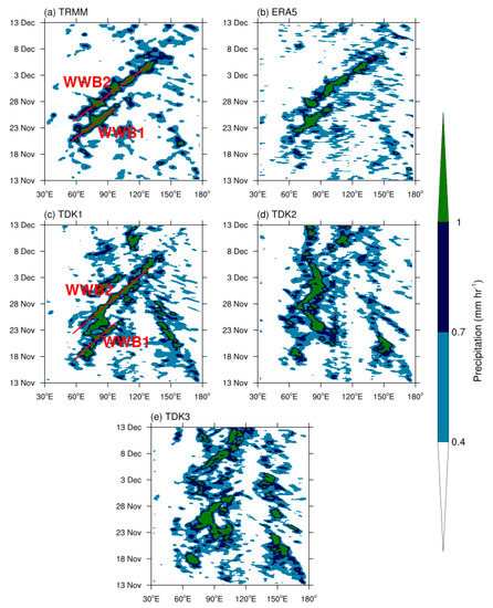
Figure 1.
Longitude-time sections of 3-hourly precipitation (mm h−1) derived from (a) TRMM satellite observation, (b) ERA5, (c) TDK1, (d) TDK2, and (e) TDK3 experiment from 13 November to 12 December 2011. Data are averaged between 10° N and 10° S. Red lines represent the first and second precipitation events (i.e., WWB1 and WWB2).
Jia et al. [36] found that the model resolution is an important factor in simulating the MJO, and that model resolution can substantially affect the simulated MJO in certain aspects. High-frequency disturbances were weaker and the structures of the simulated MJO were better defined to a certain extent at a lower horizontal resolution. A more realistic spatiotemporal spectrum and spatial distribution of MJO precipitation are associated with a higher vertical resolution. Meanwhile, increasing the model’s resolution improved the simulation of the climatology. This motivates us to construct a model with high vertical and horizontal resolutions.
This study complements a companion publication that documents a coupled tropical channel model developed to forecast the MJO during the DYNAMO campaign period [37]. The companion paper shows that the cumulus convective parameterization plays a crucial role in the MJO simulation over the Indian Ocean no matter which PBL scheme is selected, but its combination with the PBL scheme is important for the MJO simulation over the MC region. However, the companion paper focuses on the tropical mean state bias of SST, zonal wind, and cloud fraction associated with the selection of cumulus convective scheme. The tropical cloud radiative forcing are important problems to study in the MJO simulation. The focus of this study is to evaluate the impact of the PBL schemes on forecasting the eastward-propagating and non-propagating MJO precipitation events over the MC. Section 2 briefly describes the coupled tropical channel model and data used in this study. The observed and simulated MJO features, the sensitivity of MJO prediction to PBL schemes, as well as the underlying mechanisms of the MJO propagation are presented in Section 3. In Section 4, the conclusions and discussion are provided.
2. Model and Data
We utilize the Coupled Ocean–Atmosphere–Wave–Sediment Transport (COAWST) modeling system [38] to perform our numerical simulations. It is noted that the COAWST is designed for the tropical cyclone, and it is the first time for the COAWST to study the MJO with a tropical channel model domain. The COAWST model system is made up of several components, including the Regional Ocean Modeling System (ROMS), the Weather Research and Forecasting Model (WRF), the Simulating Waves Nearshore, and the Community Sediment Transport Model. The release of WRF is 3.7, and the coupled WRF-ROMS version of COAWST is used, without wave and sediment components. In this coupled version, a coupler is provided by the Model Coupling Toolkit to exchange data fields between the WRF model and the ROMS model. On the air–sea interface, near-surface meteorological fields are provided to the oceanic component by the atmospheric component. Subsequently, the momentum, water, and heat fluxes are calculated by the bulk aerodynamic formula in the oceanic component [39]. Meanwhile, the oceanic component provides only SST data to the atmospheric component.
Time-varying lateral boundary conditions contain multi-scale perturbations, which may prevent the MJO initiation and propagation [40]. To decrease the influence of time-varying lateral boundary conditions on the MJO, the typical meridional extent of the MJO envelope needs to be taken in the MJO simulation. Thus, our coupled model is configured as a periodical tropical channel with southern (31° S) and northern (39° N) boundaries away from the typical MJO meridional extent. There is no damping applied to the northern and southern boundaries. Both atmospheric and oceanic components have a horizontal grid spacing of 30 km and 40 vertical levels. About 6–8 levels are in the top 1 m of the upper ocean, and 15 levels are in the top 20 m, contributing to representing the shallow diurnal mixed layer. Air-sea coupling frequency is 10 min. This high-frequency air–sea coupling could improve the reproducibility of the intensity and temporal variation in both diurnal convection and upper-ocean processes. Six-hourly atmosphere outputs of the National Centers for Environmental Prediction (NCEP) Final Operational Global Analysis (FNL) are used to construct the initial fields and boundary conditions of the atmosphere component and the oceanic component utilizes daily ocean outputs of the Hybrid Coordinate Ocean Model (HYCOM) ocean analysis, respectively [41,42]. More details on the coupled tropical channel model can be found in the companion paper [37].
Three different PBL schemes can be selected in the WRF model. They are the University of Washington (UW) scheme [43], the Mellor–Yamada–Janjic (MYJ) scheme [44,45,46], and the Yonsei University (YSU) scheme [47]. The UW and MYJ schemes depend on local turbulent kinetic energy, while the YSU scheme depends on nonlocal mixing in the unstable mixed layers. All the model experiments use the same cumulus parameterization scheme—the Tiedtke scheme (TDK)—which has been widely used in weather and climate model simulations associated with the MJO. This cumulus scheme is based on principles of mass flux with a convective available potential energy-removal time scale and considers the shallow component and the convective momentum transport [48]. The single-moment six-class microphysics scheme [49], the Monin–Obukhov-–Janjic surface layer scheme [50], the Rapid Radiation Transfer Model [51], and the Goddard scheme [52] for longwave and shortwave radiation transfer through the atmosphere, are kept the same in the atmospheric components. The land surface process is controlled by the Noah land surface model [53]. Meanwhile, for the ocean component, the configurations are also kept unchanged in all three experiments. The K-profile parameterization scheme is used in the mixed-layer dynamics [54]. The optical classification of water is the first type, assuming it is the most transparent water suitable for the open ocean.
In this study, 30-day (from 13 November to 13 December 2011) hindcast experiments are conducted to investigate the MJO signals during the DYNAMO campaign. The same initial fields with FNL and HYCOM data are used in all 30-day hindcast experiments to explore the effects of possible physical processes associated with the PBL schemes on the MJO propagation. These experiments with a realistic earth’s terrain do not have waves and sea spray, named TDK1 (with the UW scheme), TDK2 (with the MYJ scheme), and TDK3 (with the YSU scheme). The model experiments are verified based on the data from the satellite-observed Tropical Rainfall Measuring Mission (TRMM) 3B42RT precipitation product [55], the fifth-generation European Centre for Medium-Range Weather Forecasts reanalysis (ERA5) dataset [56], and the National Oceanic and Atmosphere Administration (NOAA) Outgoing Longwave Radiation (OLR) [57].
3. Results
3.1. MJO Events
3.1.1. MJO Precipitation
To evaluate the characteristics of MJO precipitation events during the DYNAMO period, the 3-hourly precipitation from the TRMM observation, the ERA5 reanalysis, and the model hindcast experiments are averaged over 10° N–10° S (time-longitude sections in Figure 1). Two convective precipitation events are identified in the TRMM observation (Figure 1a). The two precipitation events associated with zonal westerly wind anomalies are defined as westerly wind burst 1 (WWB1) and westerly wind burst 2 (WWB2), following Moum et al. [58]. The WWB1 and WWB2 initiate around 60° E on the day 21 and 25 of November 2011, respectively. The WWB1 is blocked by the MC barrier effect, but the WWB2 moves further eastward to the equatorial western Pacific Ocean. The moving rate at around 8.6 m s−1 in TRMM is consistent with the measurements during the DYNAMO campaign [58]. These features of the two MJO precipitation events in TRMM are captured in the ERA5 (Figure 1b), and we choose this reanalysis product for diagnosis and model validation of the physical processes related to the MJO propagation [37].
The sensitivity of the eastward-propagating precipitation events to the PBL schemes is shown in three model experiments (Figure 1c–e). The three model experiments can capture the two eastward-propagating precipitation events (>1 mm h−1) over the Indian Ocean before 28 November 2011. And the WWB2 convection passing through the MC is simulated in the TDK1 experiment. However, the WWB2 convection is blocked over the MC in the TDK2 and TDK3 experiments with different PBL schemes; little precipitation signals are found at the east of the MC region. According to the moist-mode theory, the impact of the PBL scheme on the MJO simulation depends on the simulation of the atmospheric moisture.
3.1.2. MJO Phase
The differences in the initiation, propagation, and intensity of the MJO in the three model experiments are examined by using the OLR MJO index (OMI) [59]. The OMI is freely available for download from the NOAA Earth System Research Laboratory (https://psl.noaa.gov/mjo/mjoindex/ accessed on 22 October 2021). It is based on the empirical orthogonal function (EOF) analysis of bandpass-filtered OLR from 20° S to 20° N. For each of the three experiments, OLRs are projected onto the corresponding spatial EOFs associated with that day of the year to get the time series of two principal components (PC1 for the x-axis and PC2 for the y-axis in Figure 2) [59]. The daily amplitude of the MJO, or the MJO intensity, is defined as the square root of the sum of the two leading PCs squared (). The PCs are also normalized by the standard deviation of PC1 (245.642 W m−2) calculated from the Interpolated NOAA OLR.

Figure 2.
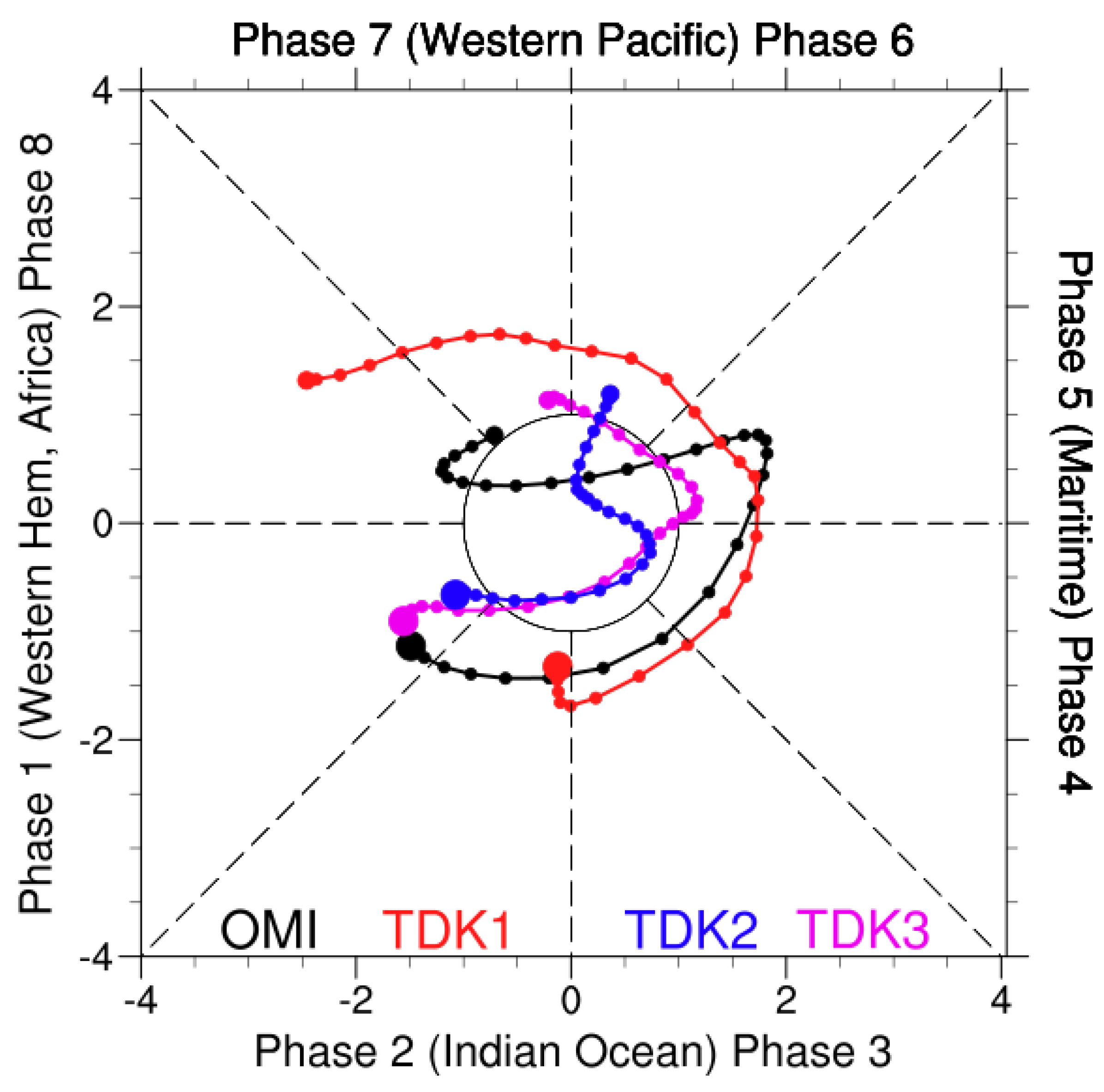
Phase diagram of OMI (black line), TDK1 (red line), TDK2 (blue line), and TDK3 (purple line) from 13 November to 13 December 2011. The dates divisible by 1 are labeled using the points. Colored lines represent different model results. The principal components (PCs) of the model results are normalized by the standard deviation (245.642 W m−2) of PC1 based on NOAA OLR.
The MJO phase diagram is shown in Figure 2. The daily amplitude of the MJO in the TDK1 experiment (red line) is similar to the OMI derived from the Interpolated NOAA OLR (black line) with . The big points represent the initial date. However, the amplitude in the other two model experiments from phase one to phase eight is too small with . This suggests the better performance of the TDK1 experiment in simulating MJO intensity. Note that the initial location of MJO in the TDK1 experiment is not near Africa in phase one, but over the Indian Ocean in phase two because the OMI is just used to estimate OLR characteristics of the MJO signals. The aforementioned results suggest that the PBL scheme appears to play a crucial role in simulating the MJO event passing through the MC.
3.2. Background Fields
3.2.1. Horizontal Structure
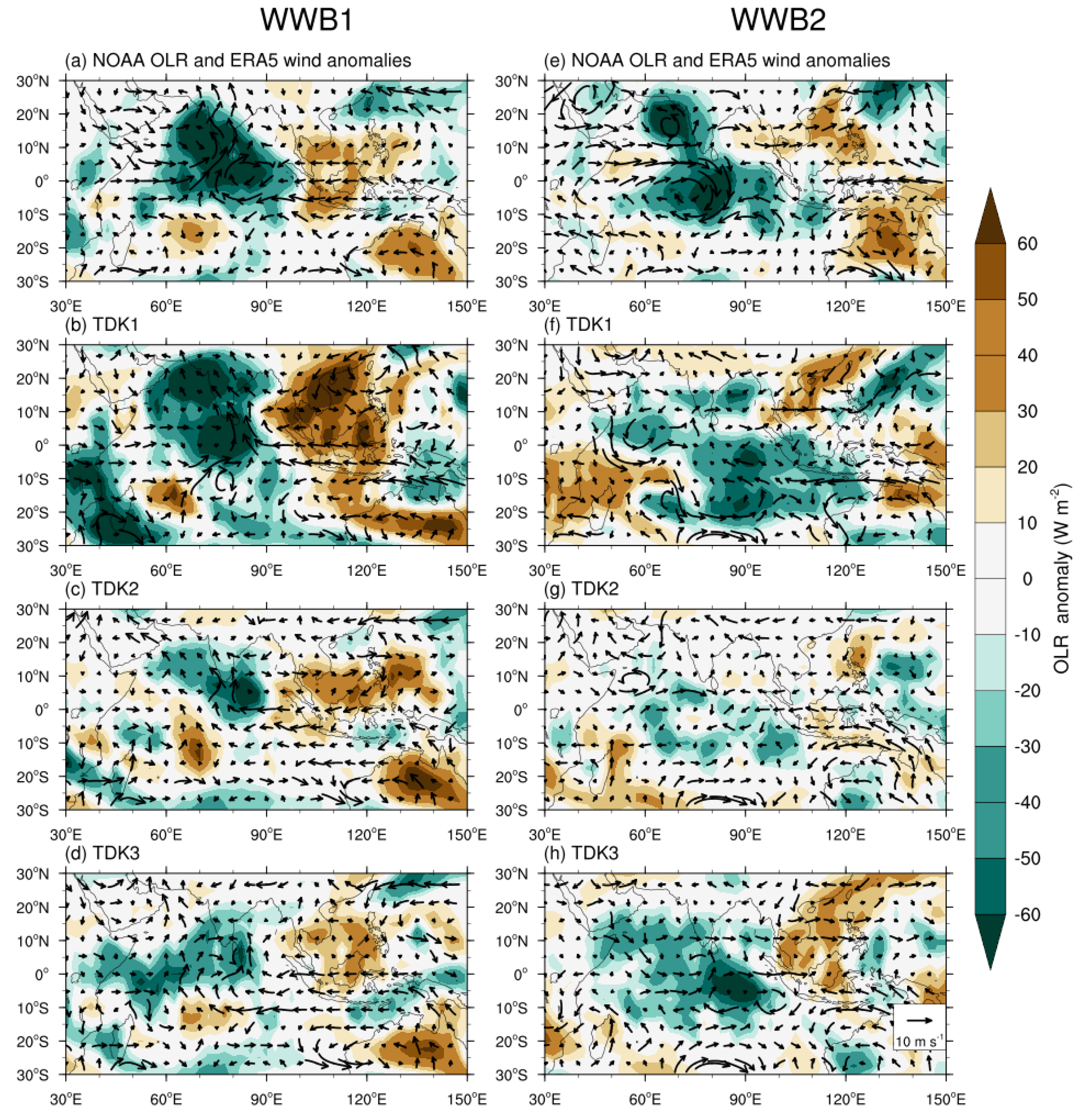
Why is the MJO precipitation zone maintained when crossing the MC in the TDK1 experiment, but it rapidly decays in the other two experiments? The west–east asymmetric moisture distribution in the numerical model has been highlighted as a key aspect in affecting the MJO propagation through the MC [60]. To investigate the reasons responsible for the parameterization’s difference, we first examined the horizontal circulation and OLR anomalies. According to the previous studies, the PBL convergence can accumulate moisture in the lower troposphere, increase the low-level MSE and destabilize the low troposphere [60]. Figure 3a shows two-day averaged horizontal OLR anomalies in the NOAA product and 850 hPa wind field anomalies in the ERA5 reanalysis. The selected date range of the WWB1 is 22 to 23 November 2011 when the convective center of the MJO precipitation event is located near 90° E in the ERA and three experiments. But for the WWB2, the time range is 27 to 28 November 2011 in the reanalysis product and the TDK1 experiment and 28 to 29 November 2011 in the TDK2 and TDK3 experiments.
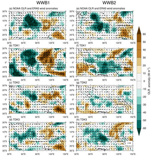
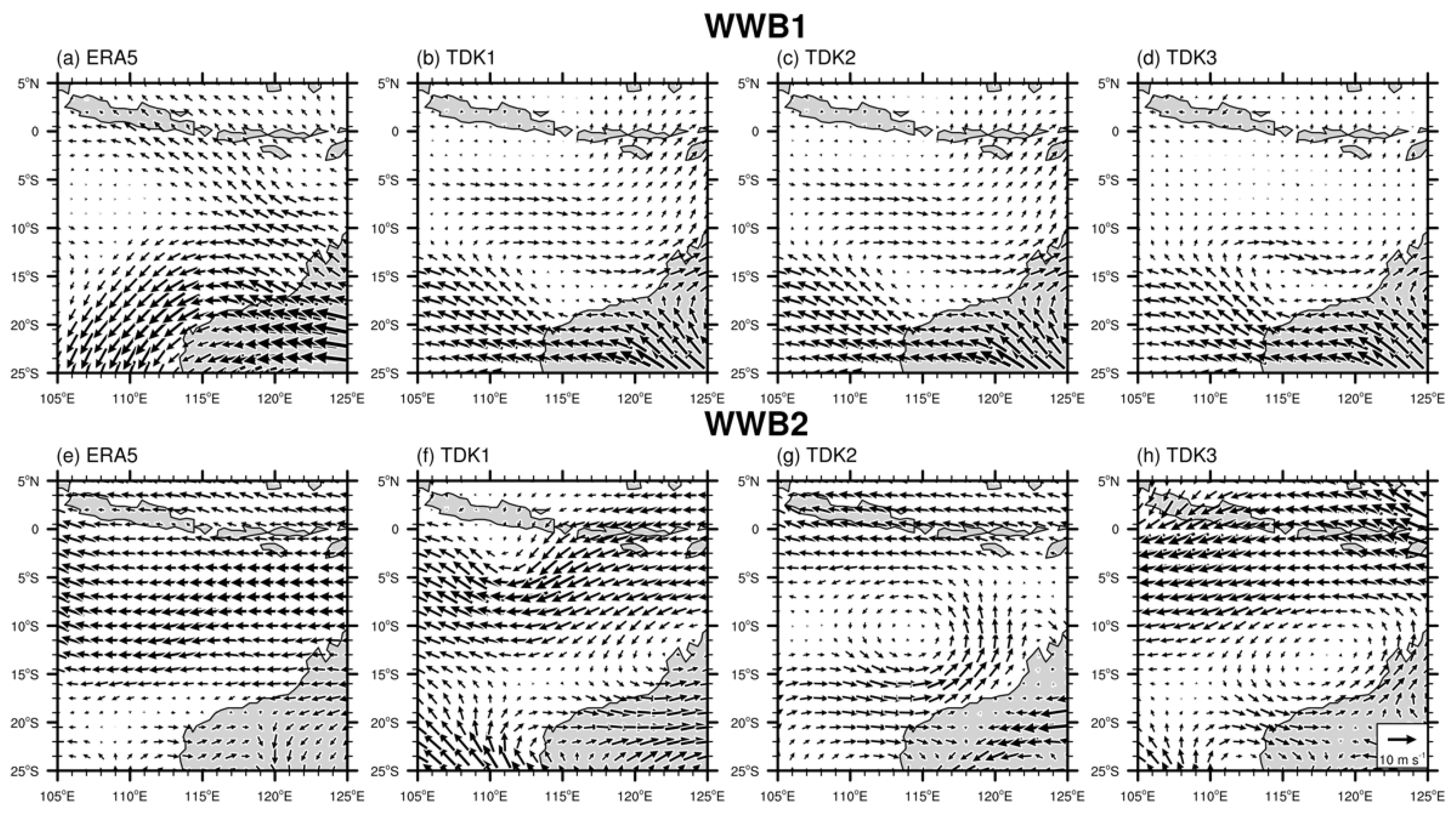
Figure 3.
Horizontal structure of the two MJO events. Composite 850 wind anomalies (vectors, 10 m s−1) are derived from (a,e) ERA5, (b,f) TDK1, (c,g) TDK2, and (d,h) TDK3. Two-day averaged results are shown in the left (right) panels when the WWB1 (WWB2) convective center is located near 90° E. The selected time range of the WWB1 is 22 to 23 November 2011. For the WWB2, the time range is 27 to 28 (28 to 29) November 2011 in the ERA5 and the TDK1 (the TDK1 and TDK2 experiments). The shading indicates the OLR anomaly (W m−2). NOAA OLR anomaly (shading, W m−2) is displayed in (a,e). ERA5 product and model results have been interpolated to the coarser resolution of NOAA OLR.
It is noted that the horizontal OLR anomaly is derived from the NOAA product and the horizontal wind field anomaly is derived from the ERA5 reanalysis. The convection of an active MJO phase is present in 60–90° E with a strong wind convergence at 850 hPa in the WWB1 (Figure 3a) and the WWB2 (Figure 3b). At this point, westerly wind anomalies exist over 45–75° E and easterly wind anomalies exist over the MC, especially over the northern ocean of the MC. An interesting wind circulation anomaly is seen at 850 hPa. The WWB1 and WWB2 feature a strong Rossby wave response to the west of the MJO convection and a weak Kelvin wave response to the east of the MJO convection [3].
For the non-propagating WWB1, negative OLR anomalies are found over the MC, which means that convection ahead of the MJO convection is not developed (see Figure 3a–d). This weak convection activity is unfavorable for maintaining the eastward propagation of the MJO across this region. However, for the eastward-propagating WWB2 in the ERA5 reanalysis, the intensity of convection over the land and ocean near Java Island is stronger than that in the WWB1 (Figure 3a vs. Figure 3e). The TDK1 experiment has a good performance in simulating the strong convection activity (Figure 3f). In contrast, both the TDK2 and TDK3 experiments do not capture strong convection with a negative OLR anomaly over the western MC (Figure 3g,h). Instead, it is similar to the atmosphere condition during the period of WWB1. The weak convection activity over the western MC in the TDK2 and TDK3 experiments may be the reason for the non-propagating MJO in the WWB2.
3.2.2. Vertical Structure
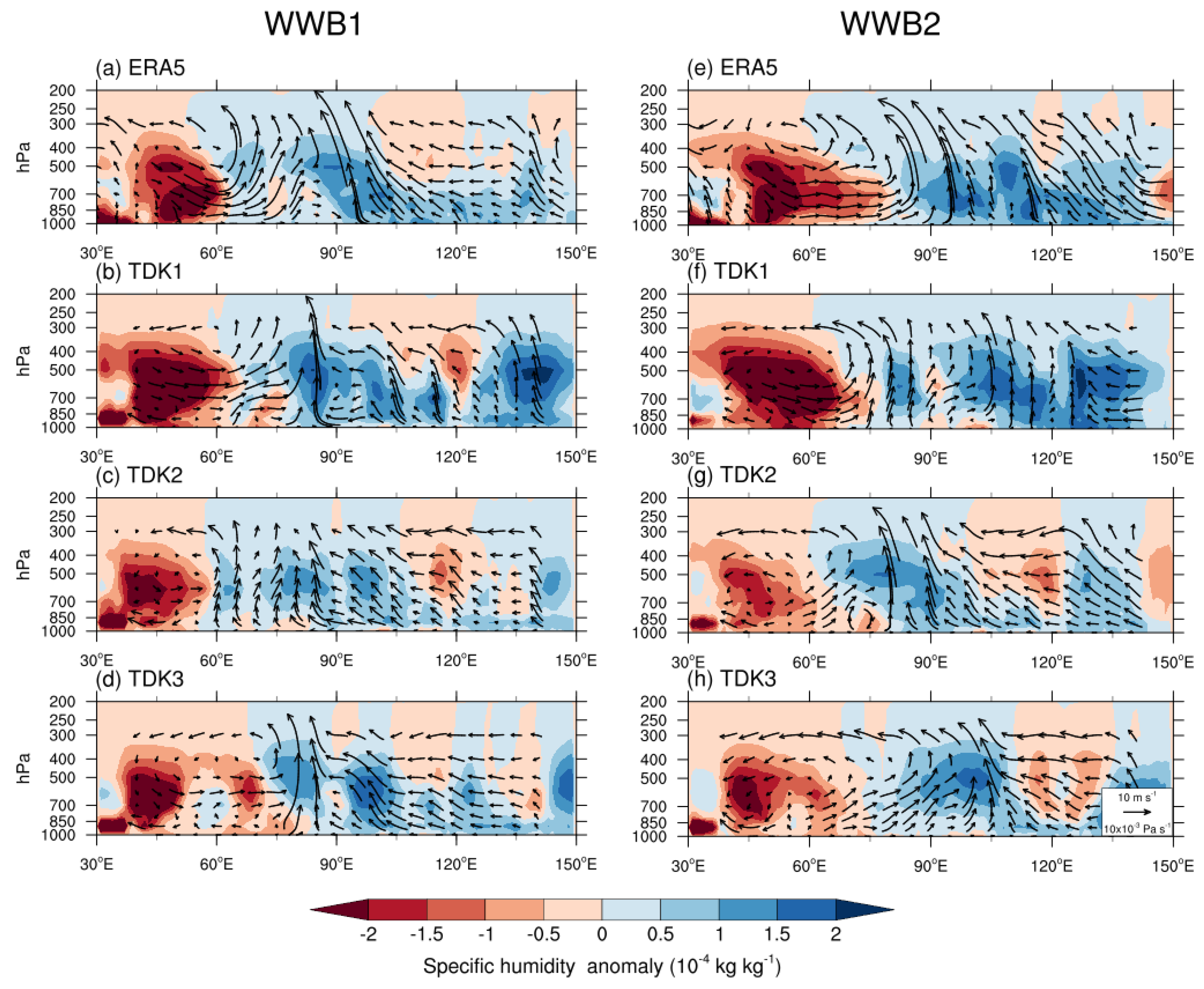
The vertical moisture structure also shows pronounced differences among the ERA5 reanalysis and the three TDK experiments, consistent with those in the east–west asymmetric circulation patterns. The specific humidity anomaly represents the change of the moisture, a variable that is central to the MJO. In Figure 4, the averaged specific humidity in each level is removed from the specific humidity to get the anomaly. The shadings in Figure 4a–d show that, for the WWB1, a positive specific humidity anomaly extends from the maximum center (around 90° E) downward and eastward to 150° E with an easterly winds profile in the vertical direction. This non-propagating MJO precipitation event is characterized by a negative specific humidity in the middle–upper troposphere from 105° E to 120° E. This dry atmospheric condition contributes to blocking MJO precipitation signals over the MC.
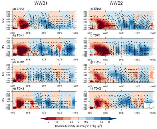
Figure 4.
Vertical structure of the two MJO events. Composited zonal (10 m s−1) and vertical (−10 × 10−3 Pa s−1) winds for (a,e) ERA5, (b,f) TDK1, (c,g) TDK2, and (d,h) TDK3. Two-day averaged results are shown in the left panels (right) panels when the WWB1 (WWB2) convective center is located near 90° E. The selected time range of the WWB1 is 22 to 23 November 2011. For the WWB2, the time range is 27 to 28 (28 to 29) November 2011 in the ERA5 and the TDK1 (the TDK1 and TDK2 experiments). The shading indicates the specific humidity anomalies (10−4 kg kg−1). The mean value of the specific humidity for each level is removed from the specific humidity to get the anomaly.
The right column of Figure 4 shows the vertical structure of the WWB2 at the point that the MJO convective center is located near 90° E. This eastward-propagating event is characterized by positive middle-level specific humidity anomalies with a strong ascending motion around the MC (Figure 4e,f). The moisture in the low-level troposphere can be transported into the middle troposphere. However, for the TDK2 and TDK3 experiments, the dry condition of the middle troposphere still influences the MC region, leading to a non-propagating MJO convection in the WWB2 (Figure 4g,h). Figure 4 indicates that correctly capturing moisture distribution features in the middle level around the MC may be necessary for a realistic MJO simulation across the MC.
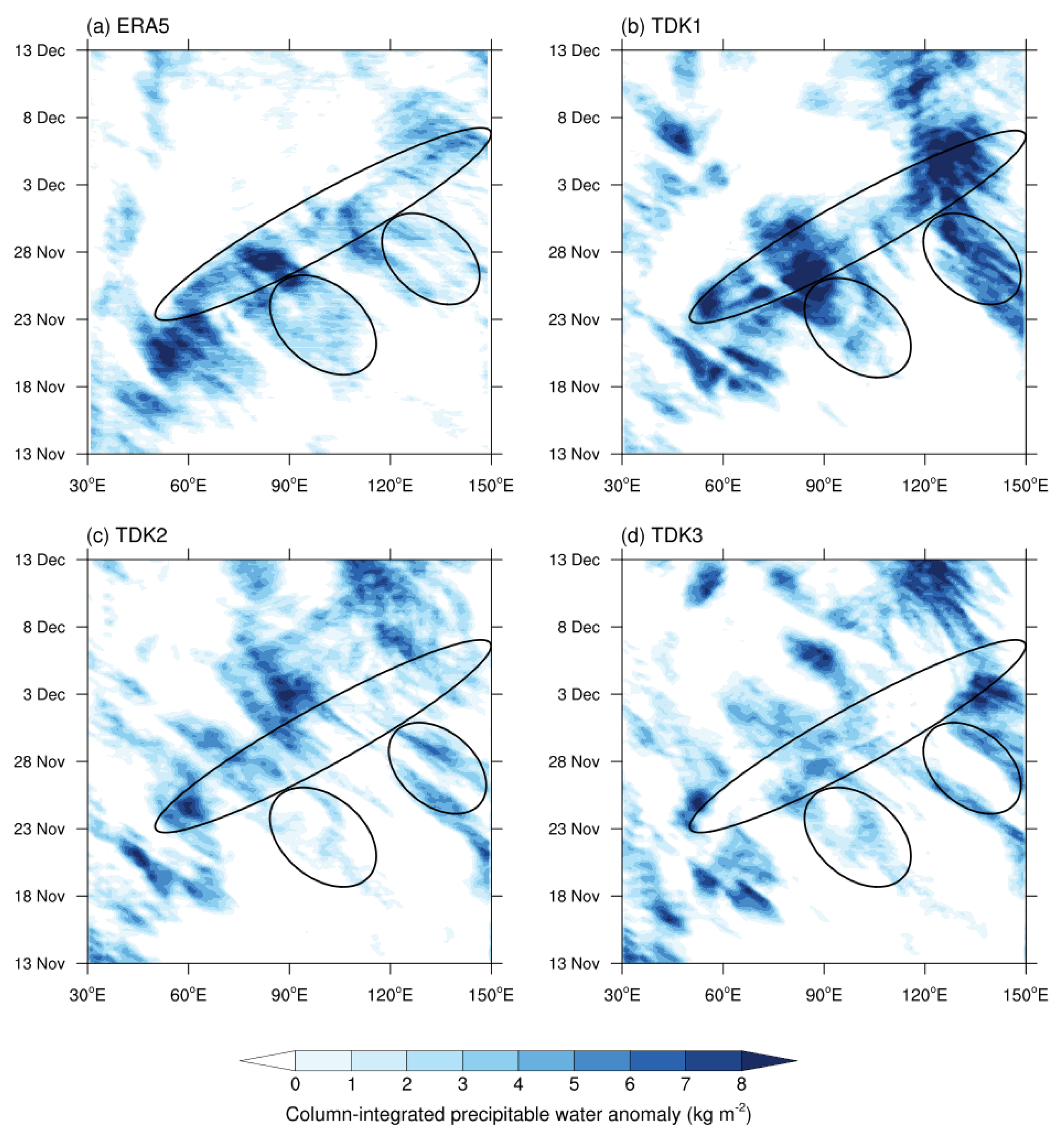
The atmospheric water cycle is central to many fundamental processes in the earth’s system. Planetary-scale patterns of water vapor play critical roles in the MJO event in both observations and simulations [61,62]. According to the vertical column-integrated precipitable water anomaly in Figure 5a,b, the simulated precipitable water anomaly is much higher in the TDK1 experiment than that in the reanalysis product. This is due to the convection trigger function in the cumulus scheme if a proper PBL scheme is selected. When the column-integrated moisture convergence exceeds the boundary layer turbulent moisture flux by 110%, deep or penetrative convection is activated in the TDK scheme. The total moisture supply from surface evaporation and large-scale convergence is assumed to go into deep convection until deep or penetrative convection is activated [63]. Thus, the positive precipitable water anomaly is overestimated. For the ERA5 reanalysis and the TDK1 (Figure 5a,b), the atmosphere is relatively dry over most of the equatorial Indian Ocean and the MC before the initial date of WWB1 (18 November). The exceptions are two subsequent moisture corridors (black circles in Figure 5a). The first one is over the central and eastern Indian Ocean in the early stages (18 to 28 November) of the WWB1, and the second one is over 60–120° E and the Western Pacific Ocean in the middle period (23 November to 3 December) of the WWB2. Heavy rainfall occurs in these moisture corridors (Figure 1, red lines), which is the manifestation of the MJO events in the precipitation field. A water vapor transport signal appears along 120° E to 90° E from 18 to 25 November, while another signal is along 150° E to 120° E from 23 November to 1 December (small circles in Figure 5a). The atmosphere over the MC region around 120° E is too dry before 28 November (in the WWB1) until the latter signal appears (in the WWB2). This water vapor difference is the reason for the different propagation progress of the WWB1 and WWB2 over this region.

Figure 5.
Longitude-time sections of 3-hourly column-integrated precipitable water anomaly (kg m−2) from (a) ERA5, (b) TDK1, (c) TDK2, and (d) TDK3 experiment from 13 November to 12 December 2011. Data are averaged between 10° N and 10° S with the time average removed. Black circles in (a) represent the propagations of column-integrated precipitable water anomaly from the ERA5.
For the TDK2 and TDK3 experiments, the atmosphere in the MC region around 120° E is always dry before 3 November (Figure 5c,d). In the TDK2 experiment, the water vapor is hard to collect in the MJO envelope (see the big circle of Figure 5c,d). An apparent jump of a positive precipitable water anomaly appears in this region as the MJO precipitation moves from the eastern Indian Ocean to the western Pacific across the MC in the TDK3 experiment. Such jumpy behavior over the MC demonstrates the sensitivity of the simulated water cycle to the PBL parameterization schemes. Ulate et al. [62] found similar results in this region. When the YSU and MYJ PBL schemes are used, dry biases produced by the PBL scheme can penetrate the middle troposphere but disappear when the UW scheme is used.
3.3. MSE Budget
It is noted that the positive MSE tendency ahead of the MJO convective center is crucial for the eastward propagation of the MJO [27]. The MSE is a thermodynamic variable that describes the state of an air parcel. It is similar to the equivalent potential temperature. As mentioned in Yano and Ambaum [64], MSE is a useful quantity in understanding moist convection, and it is conserved under moist adiabatic processes and hydrostatic balance.
The MSE is regarded as the sum of dry static energy (DSE) and Latent Static Energy (LSE). Following Yano and Ambaum [64], the DSE and LSE are defined as
and
where Cp is the specific heat of dry air at a constant pressure (J K−1 kg−1), t is the temperature (K), g is the gravity acceleration (9.8 m s−2), z is the elevation above the ground (m), Lv is the latent heat of the vaporization of water (J kg−1), and q is the specific humidity (kg kg−1).
Wang et al. [28] found that the longitudinal and latitudinal range of the analysis domain over the MC and the positions of the boundaries should be carefully designed to get the accurate contribution of each MSE budget term. Figure 6 shows the zonal distribution of the column-integrated MSE tendency averaged over 10° S–10° N for the WWB1 and WWB2. The data are derived from the two-day average of the MSE tendency, and the time range is similar to that given in Section 3.2.1. The dry air intrusion effect is found in the column-integrated MSE tendency profiles (Figure 6a) in the WWB1 because the MSE tendency is near zero or negative from 105° E to 120° E (grey shading) ahead of the MJO convection. It prohibits the development of new convection to the east of the existing convective center of the MJO. In contrast, a positive MSE tendency appears in the WWB2 over the same longitudinal band and the MSE tendency between 90° E and 105° E is negative in the ERA5 (Figure 6b, bold line). This favors the continuous eastward-propagating MJO due to the west–east asymmetric MSE tendency. The TDK1 realistically reproduces a similar MSE tendency both in the WWB1 and the WWB2 (Figure 6, thin lines). The positive MSE tendency in the WWB2 over 105–120° E supports the eastward propagation of the MJO. In contrast, the negative MSE tendencies in both WWB1 and WWB2 over the MC in the TDK2 and TDK3 experiments prohibit the MJO propagation across the MC.
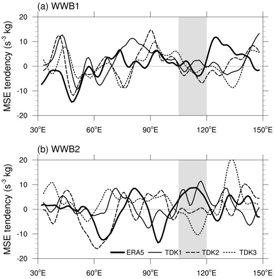
Figure 6.
Zonal distribution of the column-integrated MSE tendency (W m−2) averaged over 10° S–10° N from the ERA5 and three TDK experiments. Two-day averaged results are shown by black lines when the (a) WWB1 and (b) WWB2 convective centers are near the 90° E. The gray shaded area represents the analysis domain between 105° E and 120° E.
Figure 7 illustrates the time evolutions of the vertical distribution of MSE, DSE, and LSE over the analysis domain of the MC (10° N–10° S, 105–120° E) from the ERA5 reanalysis and the three forecast experiments. In the lower troposphere, the MSE starts to increase on 18 November, but the atmosphere is still dry above the PBL before 23 November, especially in the 400–500 hPa levels (Figure 7a). The lack of moisture in the vertical direction weakens the cloud–radiation effect and is not able to locally warm the troposphere; the cloud–radiation effect is essential to convection development [65]. This is the reason for the non-propagating MJO precipitation in WWB1. After 23 November, the increase in MSE in the troposphere at 1000–200 hPa over the MC leads to the eastward-propagating MJO in the WWB2. These different characteristics of MSE distribution between the WWB1 and the WWB2 are realistically captured in the TDK1 experiment (Figure 7b). Interestingly, the increase in MSE in the lower-middle troposphere is not reproduced in the TDK2 and TDK3 experiments before 28 November when the second MJO precipitation event is located near the MC (Figure 7c,d). The MSE (first column) is primarily regulated by the DSE (second column) in the middle-upper troposphere as a result of temperature anomalies but is mainly regulated by the LSE (third column) in the lower-middle troposphere as a result of latent heat flux anomalies. The increases of DSE in the upper troposphere at 450–200 hPa (Figure 7e) and LSE in the lower troposphere at 1000–850 hPa (Figure 7i) are realistically captured in the TDK1 experiment (Figure 7f,j). In contrast, the upper-level DSE and lower-level LSE in the TDK2 and TDK3 experiments are small (Figure 7g,k,h,l), which means that the moisture from the PBL to the free atmosphere is regulated by the PBL schemes.
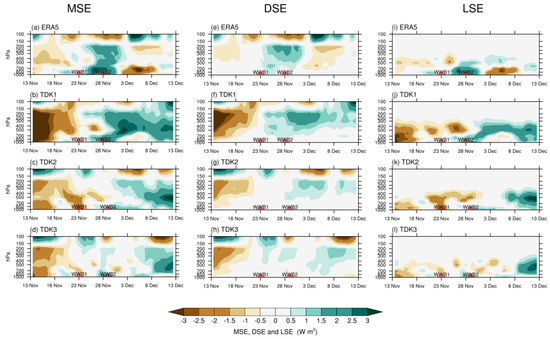
Figure 7.
Time-pressure diagrams of the MSE (left panels, W m−2), the DSE (middle panels, W m−2), and the LSE (right panels, W m−2) over the analysis domain (10° N–10° S, 105–120° E) derived from (a,e,i) ERA5, (b,f,j) TDK1, (c,g,k) TDK2, and (d,h,l) TDK3 between 13 November and 13 December 2011. The red triangles present the time ranges when the WWB1 and WWB2 convective centers are located near the 90° E.
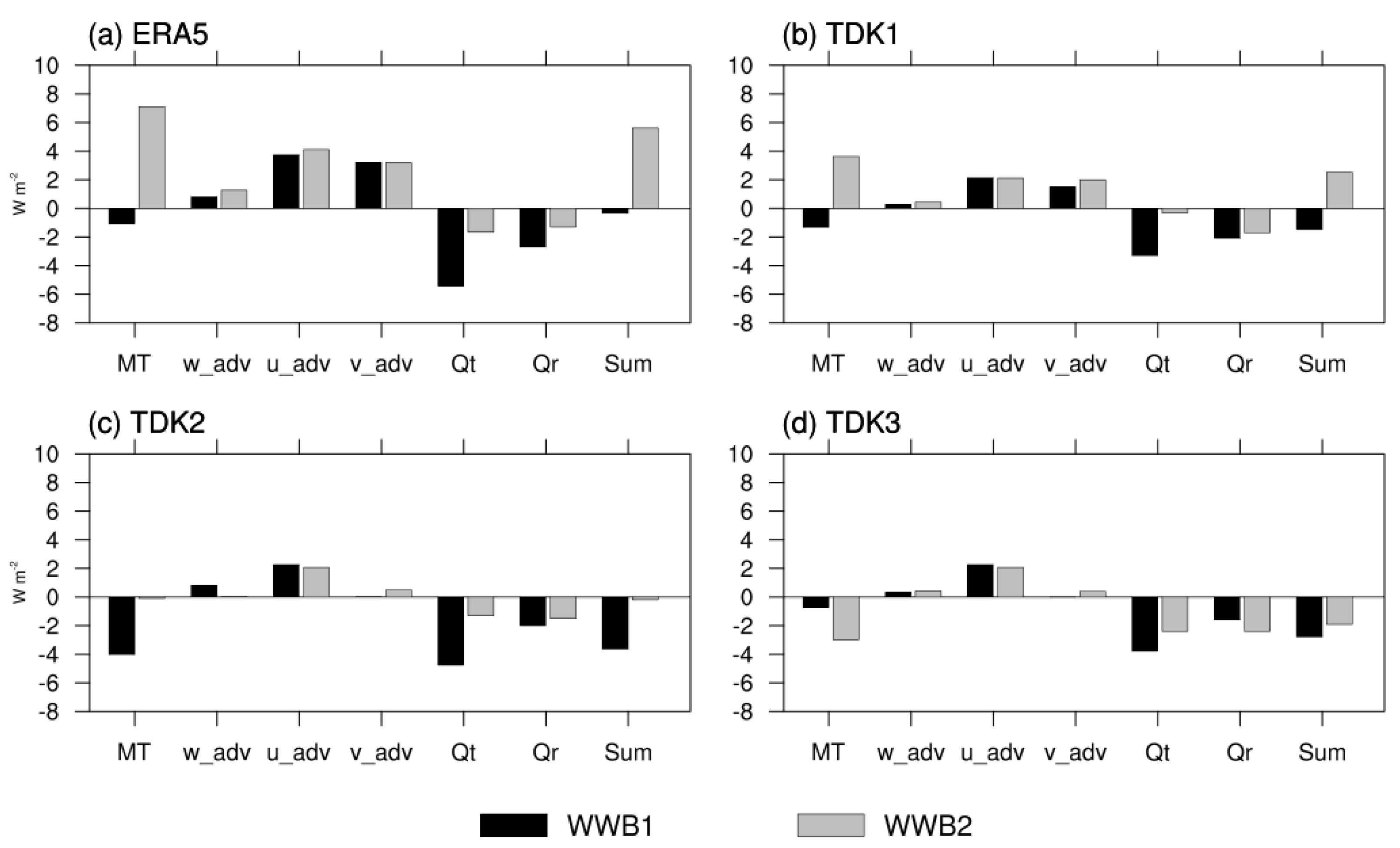
To further evaluate the processes relating to the moisture and the intensity of MJO convection, an MSE budget analysis has been performed. As in Neelin and Held [66] and Maloney [17], the MSE budget can be written as:
and
where represents the MSE tendency (MT, W m−2). On the right-hand side, the first term in Equation (3) represents the transport of MSE due to the vertical velocity (w_adv, W m−2). The is the vertical pressure velocity (Pa s−1) and p is the pressure (Pa). The second term represents the transport of MSE due to the horizontal advection, which can be divided into zonal (u_adv, W m−2) and meridional advection terms (v_adv, W m−2) as displayed in Equation (4). is the horizontal wind vector. The surface turbulent heat flux (Qt, W m−2) includes the surface latent (LH) and sensible (SH) heat flux. The column-integrated radiation heat rate (Qr, W m−2) contains the vertically integrated longwave (LW) and shortwave (SW) heating rates. The Qt and Qr are determined by LH and LW with an order of magnitude larger than and SW, respectively.
The spatial average in the domain of 105–120° E and 10° N–10° S is computed for the budget term in Equation (3) and displayed in Figure 8. The horizontal advection and vertical advection (u_adv, v_adv, and w_adv) increase the MSE over 105–120° E with a large contribution from the horizontal advection in the ERA5 reanalysis (Figure 8a). The turbulent heat flux (Qt) and the radiation heating rate (Qr) decrease the MSE. For the non-propagating WWB1, the five terms in the total lead to a negative MSE tendency. In WWB2, the heat produced by the horizontal and vertical advection slightly increased and the heat moved away by turbulent and radiation heat flux decreased, contributing to the increased MSE. These contributions are realistically reproduced in the TDK1 experiment despite that the absolute values are smaller in the TDK1 than in the ERA5. The meridional advection term (v_adv) in the TDK2 and TDK3 experiments is much smaller than that in the TDK1. The lack of heat and water vapor transported from the extratropics to the tropics is responsible for the non-continuous propagation of MJO convection across the MC in the TDK2 and TDK3 experiments.

Figure 8.
Fractional contributions of each MSE budget component to the east–west asymmetric MSE tendency pattern over the study domain (10° N–10° S, 105–120° E) for (a) ERA5, (b) TDK1, (c) TDK2, and (d) TDK3 experiment. Black boxes (gray boxes) are two-day averaged results when the WWB1 (WWB2) convective center is located near 90° E. The bars from left to right represent the MSE tendency (MT), the vertical MSE advection (w_adv), the zonal MSE advection (u_adv), the meridional MSE advection (v_adv), surface heat fluxes (Qt), the atmospheric radiative term (Qr), and the sum of MSE budget terms. The unit is W m−2.
3.4. Meridional Wind and Specific Humidity
To address the question of why the different experiments using different PBL schemes yield such different meridional MSE advection, time-latitude diagrams of the 850-hPa meridional wind over 105–120° E are plotted in Figure 9. From 23 to 28 November, the strong convergence of meridional wind in the tropics (marked in the red triangle, southerly wind over 0–10° S and northerly wind over 0–10° N) supported PBL moisture convergence in the ERA5 and the TDK1 experiment. However, in the TDK2 and TDK3 experiments, when the WWB2 convective center is located near the MC from 28 to 29 November, the southerly wind over the Southern Hemisphere changed to the northerly wind (Figure 9c,d). The tropical wind convergence ahead of the MJO convection is not captured in the TDK2 and TDK3 experiments with the northerly wind crossing the equator from 28 to 29 November, which tends to weaken the PBL moisture convergence for the MJO propagation. Similarly, the cross-equatorial flow is also found at 250 hPa around the same time (not shown). This means that the PBL schemes can lead to different simulated results about the meridional wind over the MC. The errors in the simulated meridional wind based on the MYJ and YSU PBL schemes lead to the bias of meridional circulation and further prohibit moisture convergence over the MC region.
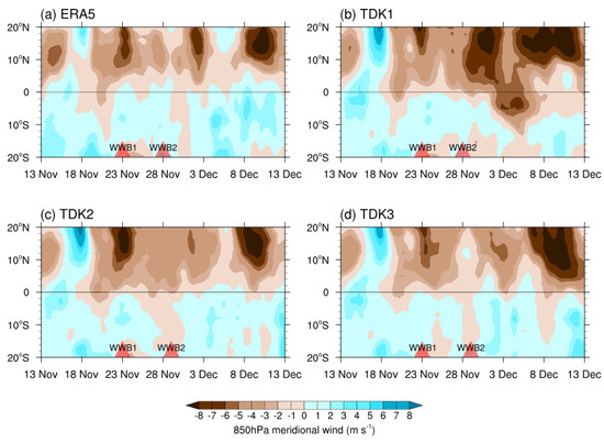
Figure 9.
Time-latitude diagrams of 850 hPa meridional wind (m s−1) over the analysis domain (10° N–10° S, 105–120° E) for (a) ERA5, (b) TDK1, (c) TDK2, and (d) TDK3 experiment from 13 November to 13 December 2011. The red triangles present the time ranges when the WWB1 and WWB2 convective centers are located near 90° E.
The 850 hPa wind vectors in the WWB1 and WWB2 from the ERA5 reanalysis and the three experiments are shown in Figure 10. For the WWB1, a wind convergence region appears over the ocean off the southwestern part of Australia in all the model experiments, which means that there are some systematic biases in the tropical channel no matter which PBL scheme is selected. This systematic bias does not influence the meridional MSE advection of the experiments in the WWB1. However, for the WWB2, an obvious anticyclone appears over this region in the TDK2 and TDK3 experiments only. If considering the cross-equatorial flow at 850 hPa (Figure 9c,d) and 250 hPa, the meridional circulation is not simulated well in the TDK2 and TDK3 experiments. This difference has also confirmed that the PBL scheme can change the tropical vapor variations via the meridional wind.

Figure 10.
Horizontal circulations of 850 hPa winds (m s−1, vectors) for (a,e) ERA5, (b,f) TDK1, (c,g) TDK2, and (d,h) TDK3 experiments. The upper (bottom) panels display two-day averaged results when the WWB1 (WWB2) convective center is located near 90° E. The shading represents the land.
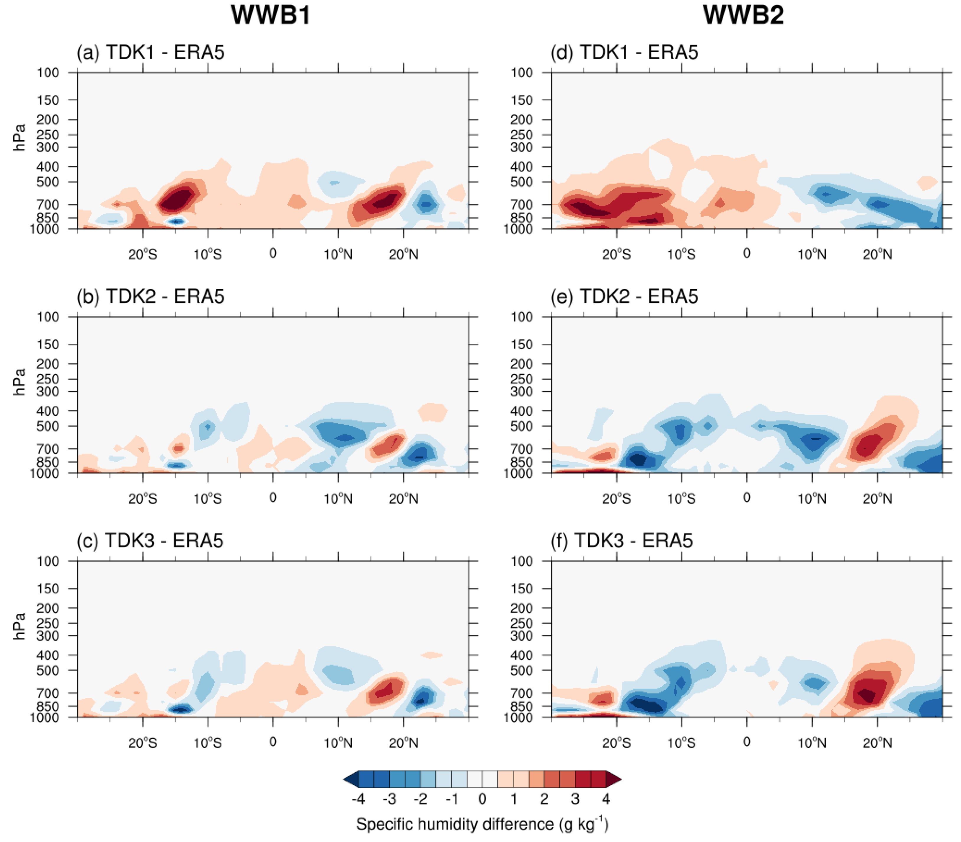
To further illustrate the impacts of the different PBL schemes on the water vapor forecasts, Figure 11 shows pressure-latitude diagrams of the specific humidity difference between all experiments and the ERA5 reanalysis. Considering the overestimation of the column-integrated precipitable water anomaly in Figure 5b, we find that there is a low-level wet bias over the tropics in the TDK1 experiment, especially over the Southern Hemisphere in the WWB2. The middle-level troposphere is much drier on both sides of the analysis domain (105–120° E, 10° N–10° S) in the TDK2 and TDK3 experiments when the first convective center is located near 90° E (Figure 11b,c). The relatively dry condition outside the analysis domain decreases water vapor flux toward the tropics despite the tropical wind convergence (Figure 9c,d), leading to the meridional MSE advection biases shown in Figure 8c,d (black boxes). The dry bias covers 10° N and 10° S in the TDK2 and TDK3 in response to the biases in the cross-equatorial flow (Figure 9c,d and Figure 11c,d). But for the WWB2, the maximum of the dry bias appears at 700–800 hPa as a result of the low-level divergence over 15° S–20° S. This dry atmospheric condition explains why the meridional MSE advection is still weak in the WWB2 (gray boxes in Figure 8c,d). Thus, a faithful simulated eastward-propagating MJO over the MC requires the correct meridional advection and water vapor transport. The PBL scheme plays a crucial role in simulating the latter two fields.
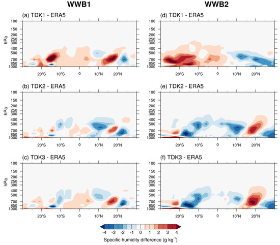
Figure 11.
Pressure-latitude diagrams of the specific humidity difference (g kg−1) between all experiments and the ERA5 reanalysis. Data are averaged between 105° E and 120° E. The left (right) panel displays two-day averaged results when the WWB1 (WWB2) convective center is located near 90° E.
4. Summary and Discussion
Based on the coupled COAWST, we designed a high-resolution tropical channel model to simulate the evolution of the MJO precipitation events over the MC during the DYNAMO campaign period. This model is periodical in the zonal direction and thereby can eliminate the spurious effects of artificial eastern and/or western boundaries. Results of the three hindcast experiments illustrate the sensitivity of MJO event simulation to PBL parameterization schemes. The three experiments use different PBL schemes (UW, MYJ, and YSU) and the same TDK cumulus parameterization scheme. The experiments with the UW PBL scheme can simulate the eastward-propagating MJO precipitation over the MC, similar to previous studies [28].
The diagnosis of model simulations indicates that the successful MJO simulation over the MC relies on the model’s capability to represent the west-east asymmetry of the MSE tendency in the equatorial zone. Our results indicate that a proper selection of the PBL scheme leads to a better simulation/forecast of the horizontal MSE advection associated with the MJO. The horizontal MSE advection over the MC regulates an increased middle-level specific humidity and recharges the MSE, forming a wet atmospheric condition favorable for the MJO propagation. The difference among the three experiments appears in the meridional MSE advection. The weak meridional MSE advection leads to a dry condition over the MC, which cannot contribute to the atmosphere moistening ahead of the MJO convection and the eastward propagation of MJO precipitation. A further diagnosis of the meridional wind shows that the model capacity in capturing the meridional circulation has an important impact on the meridional MSE advection simulation. The low-level wind circulation is not reproduced well in the failed forecasts, leading to an erroneous meridional circulation. The errors in the cross-equatorial wind can influence the tropical moisture convergence and weaken the meridional MSE advection. In addition, the well-simulated upward transport of moisture from the PBL to the free atmosphere supports the cloud-radiation effect to heat the troposphere, which is essential to set up new convection activity over the MC ahead of the MJO.
It is difficult to understand that the fundamental physics of the MJO forms the base for forecasting the MJO. Many hypotheses have been proposed to explain the dynamics of the MJO, but a single theory is difficult/has failed to explain the most fundamental characteristic of the MJO [67]. These theories have been merged to form modern theories that describe several fundamental aspects of the MJO, such as the trio-interaction theory [68]. The lack of a unified theory still restricts the improvement of the MJO forecast. So far, the moisture-mode theory may be more suitable for the MJO forecast because correcting errors in water vapor alone is necessary and sufficient for a realistic simulation of the MJO event. In another MJO event/period, the model bias may be different, including diurnal signals, latent heat flux (moisture), land surface progress, land–atmosphere interaction, MJO–wave interaction, etc. This raises a further puzzle and needs more study. In addition, the contribution of atmosphere–ocean feedback to the emergence and evolution of the MJO remains unclear, which prompted the DYNAMO. The intensive sounding observations (atmospheric and oceanic data) from DYNAMO/Cooperative Indian Ocean Experiment on Intraseasonal Variability in the Year 2011(CINDY) field campaign provides an opportunity for us to study the moistening progress of the MJO associated with the air-sea interaction. Many kinds of research have so far been provided based on the DYNAMO observations [30,57].
The vertical mixing strength of the PBL scheme plays a bigger role in modulating the temperature and moisture in the convective boundary layer [32,69]. The difference in vertical mixing strength leads to a different temperature and moisture in the PBL. Stronger vertical mixing causes stronger entrainment at the top of the PBL. The local closure models (UW and MYJ) have a stronger vertical mixing strength than the nonlocal model (MYJ). The nonlocal schemes only simulated stronger vertical mixing at nighttime, producing higher temperature and lower moisture in the convective boundary layer. Local schemes have some advantages in the prediction of wind speed and direction.
In this paper, the UW shows a stronger vertical mixing strength in the MJO event (see WWB2 in Figure 7i–l). The low-level water vapor can be transported to a higher level and moisten it, leading to uncertainty in the representation of cloud processes and their feedback on radiation. The companion paper shows a time-averaged high cloud fraction. There is a negative high cloud fraction bias over the longitude region (105–120° E) in TDK2 and TDK3 experiments [37]. This cloud fraction bias weakens the meridional temperature gradient in the ocean and atmosphere, leading to anomalous meridional MSE advection ahead of the MJO convective center.
This study offers a good opportunity for better recognizing the advantages and disadvantages of the PBL scheme on the MJO simulation. However, the non-propagation and eastward propagation of the MJO across the MC are still hard to predict because of the complex spatiotemporal variability in atmospheric moisture as a consequence of land–sea contrast, topography, surface water and energy fluxes, and atmospheric circulation. Thus, additional research is needed to reveal how to improve the PBL schemes under warm and moist regimes. To better understand the role of the PBL scheme on the evolution of the MJO across the MC, more studies will be performed over the tropical regions to compare specific parameterization processes shortly.
Author Contributions
Conceptualization, J.-J.L.; methodology, X.W.; software, Y.H.; validation, Y.H.; formal analysis, Y.H.; investigation, Y.H.; resources, X.W. and D.W.; data curation, X.L. and H.Y.; writing—original draft preparation, Y.H.; writing—review and editing, Y.H., X.W. and J.-J.L.; visualization, Y.H.; supervision, C.Y. and H.Y.; project administration, C.Y. and H.Y.; funding acquisition, J.-J.L., X.W. and X.L. All authors have read and agreed to the published version of the manuscript.
Funding
The author Y.H. was supported by the Natural Science Foundation of China (Grant Nos. 42030605, 42088101, 41906190, and 92158204) and the Strategic Priority Research Program of the Chinese Academy of Sciences (XDA20060503).
Institutional Review Board Statement
Not applicable.
Informed Consent Statement
Not applicable.
Data Availability Statement
The data of the TRMM 3B42RT precipitation product could be found at https://gpm.nasa.gov/data accessed on 5 April 2021. The data of ERA5 could be downloaded at Copernicus Climate Change Service (C3S) Climate Date Store: https://cds.climate.copernicus.eu/#!/search?text=ERA5&type=dataset accessed on 22 June 2021. The NOAA OLR data are available at https://psl.noaa.gov/data/gridded/data.interp_OLR.html accessed on 17 May 2021.
Acknowledgments
We thank the High-Performance Computing Division of the South China Sea Institute of Oceanology for supporting the numerical simulation. We thank all scientists and staff members who contribute to the observations and reanalysis of data archive.
Conflicts of Interest
The authors declare no conflict of interest.
References
- Madden, R.A.; Julian, P.R. Detection of a 40–50 Day Oscillation in the Zonal Wind in the Tropical Pacific. J. Atmos. Sci. 1971, 28, 702–708. [Google Scholar] [CrossRef]
- Madden, R.A.; Julian, P.R. Description of Global-Scale Circulation Cells in the Tropics with a 40–50 Day Period. J. Atmos. Sci. 1972, 29, 1109–1123. [Google Scholar] [CrossRef]
- Wang, B.; Chen, G.; Liu, F. Diversity of the Madden-Julian Oscillation. Sci. Adv. 2019, 5, eaax0220. [Google Scholar] [CrossRef] [PubMed] [Green Version]
- Maloney, E.D.; Sobel, A.H. Surface fluxes and ocean coupling in the tropical intraseasonal oscillation. J. Clim. 2004, 17, 4368–4386. [Google Scholar] [CrossRef] [Green Version]
- Sobel, A.; Maloney, E.D.; Bellon, G.; Dargan, M.F. The role of surface heat fluxes in tropical intraseasonal oscillations. Nat. Geosci. 2008, 1, 653–657. [Google Scholar] [CrossRef]
- Hsu, H.H.; Lee, M.Y. Topographic effects on the eastward propagation and initiation of the Madden-Julian oscillation. J. Clim. 2005, 18, 795–809. [Google Scholar] [CrossRef]
- Adames, A.F.; Kim, D. The MJO as a dispersive, convectively coupled moisture wave: Theory and observations. J. Atmos. Sci. 2016, 73, 913–941. [Google Scholar] [CrossRef]
- Feng, J.; Li, T.; Zhu, W. Propagating and nonpropagating MJO events over maritime continent. J. Clim. 2015, 28, 8430–8449. [Google Scholar] [CrossRef]
- Kim, H.M.; Kim, D.; Vitart, F.; Toma, V.E.; Kug, J.S.; Webster, P.J. MJO propagation across the Maritime Continent in the ECMWF ensemble prediction system. J. Clim. 2016, 29, 3973–3988. [Google Scholar] [CrossRef]
- Adames, Á.F.; Wallace, J.M. Three-dimensional structure and evolution of the MJO and its relation to the mean flow. J. Atmos. Sci. 2014, 71, 2007–2026. [Google Scholar] [CrossRef]
- Muhammad, F.R.; Lubis, S.W.; Setiawan, S. Impacts of the Madden–Julian oscillation on precipitation extremes in Indonesia. Int. J. Climatol. 2021, 41, 1970–1984. [Google Scholar] [CrossRef]
- Fathurochman, I.; Lubis, S.W.; Setiawan, S. Impact of Madden-Julian Oscillation (MJO) on Global Distribution of Total Water Vapor and Column Ozone. IOP Conf. Ser. Earth Environ. Sci. 2017, 54, 012034. [Google Scholar] [CrossRef]
- Ungerovich, M.; Barreiro, M.; Masoller, C. Influence of Madden–Julian Oscillation on extreme rainfall events in Spring in southern Uruguay. Int. J. Climatol. 2021, 41, 3339–3351. [Google Scholar] [CrossRef]
- Tang, Y.; Yu, B. MJO and its relationship to ENSO. J. Geophys. Res. Atmos. 2008, 113, 1–18. [Google Scholar] [CrossRef]
- Lee, R.W.; Woolnough, S.J.; Charlton-Perez, A.J.; Vitart, F. ENSO Modulation of MJO Teleconnections to the North Atlantic and Europe. Geophys. Res. Lett. 2019, 46, 13535–13545. [Google Scholar] [CrossRef] [Green Version]
- Chen, G.; Ling, J.; Li, C.; Zhang, Y.; Zhang, C. Barrier effect of the indo-pacific maritime continent on MJO propagation in observations and CMIP5 models. J. Clim. 2020, 33, 12. [Google Scholar] [CrossRef] [Green Version]
- Zhang, C.; Ling, J. Barrier effect of the Indo-Pacific Maritime Continent on the MJO: Perspectives from tracking MJO precipitation. J. Clim. 2017, 30, 3439–3459. [Google Scholar] [CrossRef]
- Ahn, M.S.; Kim, D.; Kang, D.; Lee, J.; Sperber, K.R.; Gleckler, P.J.; Jiang, X.; Ham, Y.G.; Kim, H. MJO Propagation Across the Maritime Continent: Are CMIP6 Models Better Than CMIP5 Models? Geophys. Res. Lett. 2020, 47, 1–9. [Google Scholar] [CrossRef]
- Ling, J.; Zhang, C.; Joyce, R.; Xie, P.P.; Chen, G. Possible Role of the Diurnal Cycle in Land Convection in the Barrier Effect on the MJO by the Maritime Continent. Geophys. Res. Lett. 2019, 46, 3001–3011. [Google Scholar] [CrossRef]
- Seo, K.H.; Wang, W.; Gottschalck, J.; Zhang, Q.; Schemm, J.K.E.; Higgins, W.R.; Kumar, A. Evaluation of MJO forecast skill from several statistical and dynamical forecast models. J. Clim. 2010, 22, 2372–2388. [Google Scholar] [CrossRef]
- Ahn, M.S.; Kim, D.; Sperber, K.R.; Kang, I.S.; Maloney, E.; Waliser, D.; Hendon, H. MJO simulation in CMIP5 climate models: MJO skill metrics and process-oriented diagnosis. Clim. Dyn. 2017, 49, 4023–4045. [Google Scholar] [CrossRef] [Green Version]
- Lubis, S.W.; Jacobi, C. The modulating influence of convectively coupled equatorial waves (CCEWs) on the variability of tropical precipitation. Int. J. Climatol. 2015, 35, 1465–1483. [Google Scholar] [CrossRef]
- Lubis, S.W.; Respati, M.R. Impacts of convectively coupled equatorial waves on rainfall extremes in Java, Indonesia. Int. J. Climatol. 2021, 41, 2418–2440. [Google Scholar] [CrossRef]
- Peatman, S.C.; Schwendike, J.; Birch, C.E.; Marsham, J.H.; Matthews, A.J.; Yang, G. A Local-to-Large Scale View of Maritime Continent Rainfall: Control by ENSO, MJO, and Equatorial Waves. J. Clim. 2021, 34, 8933–8953. [Google Scholar] [CrossRef]
- Sakaeda, N.; Kiladis, G.; Dias, J. The Diurnal Cycle of Rainfall and the Convectively Coupled Equatorial Waves over the Maritime Continent. J. Clim. 2020, 33, 3307–3331. [Google Scholar] [CrossRef]
- Sobel, A.; Maloney, E. An idealized semi-empirical framework for modeling the Madden-Julian oscillation. J. Atmos. Sci. 2012, 69, 1691–1705. [Google Scholar] [CrossRef]
- Maloney, E.D. The moist static energy budget of a composite tropical intraseasonal oscillation in a climate model. J. Clim. 2009, 22, 711–729. [Google Scholar] [CrossRef] [Green Version]
- Wang, L.; Li, T.; Maloney, E.; Wang, B. Fundamental causes of propagating and nonpropagating MJOs in MJOTF/GASS models. J. Clim. 2017, 30, 3743–3769. [Google Scholar] [CrossRef]
- Wang, L.; Li, T. Effect of vertical moist static energy advection on MJO eastward propagation: Sensitivity to analysis domain. Clim. Dyn. 2020, 54, 2029–2039. [Google Scholar] [CrossRef]
- Jiang, X.; Adames, A.F.; Kim, D.; Maloney, E.; Lin, H.; Kim, H.; Zhang, C.; DeMott, C.; Klingaman, N. Fifty Years of Research on the Madden-Julian Oscillation: Recent Progress, Challenges, and Perspectives. J. Geophys. Res. Atmos. 2020, 125, e2019JD030911. [Google Scholar] [CrossRef]
- Hsu, P.C.; Li, T. Role of the boundary layer moisture asymmetry in causing the eastward propagation of the Madden-Julian oscillation. J. Clim. 2012, 25, 4914–4931. [Google Scholar] [CrossRef] [Green Version]
- Hu, X.M.; Nielsen-Gammon, J.W.; Zhang, F. Evaluation of three planetary boundary layer schemes in the WRF model. J. Appl. Meteorol. Climatol. 2010, 49, 1831–1844. [Google Scholar] [CrossRef] [Green Version]
- Yang, Y.M.; Wang, B. Improving MJO simulation by enhancing the interaction between boundary layer convergence and lower tropospheric heating. Clim. Dyn. 2019, 52, 4671–4693. [Google Scholar] [CrossRef]
- Yoneyama, K.; Zhang, C.; Long, C.N. Tracking pulses of the Madden-Julian oscillation. Bull. Am. Meteorol. Soc. 2013, 94, 1871–1891. [Google Scholar] [CrossRef]
- Tseng, K.C.; Sui, C.H.; Li, T. Moistening processes for Madden-Julian oscillations during DYNAMO/CINDY. J. Clim. 2015, 28, 3041–3057. [Google Scholar] [CrossRef]
- Jia, X.; Li, C.; Ling, J.; Zhang, C. Impacts of a GCM’s resolution on MJO simulation. Adv. Atmos. Sci. 2008, 25, 139–156. [Google Scholar] [CrossRef]
- Hu, Y.; Wang, X.; Luo, J.J.; Wang, D.; Yan, H.; Yuan, C.; Lin, X. Forecasts of MJO during DYNAMO in a coupled tropical channel model, Part I: Impact of parameterization schemes. Int. J. Climatol. 2022, 1–22. [Google Scholar] [CrossRef]
- Warner, J.C.; Armstrong, B.; He, R.; Zambon, J.B. Development of a Coupled Ocean-Atmosphere-Wave-Sediment Transport (COAWST) Modeling System. Ocean. Model. 2010, 35, 230–244. [Google Scholar] [CrossRef] [Green Version]
- Fairall, C.W.; Bradley, E.F.; Rogers, D.P.; Edson, J.B.; Young, G.S. Bulk parameterization of air-sea fluxes for Tropical Ocean-Global Atmosphere Coupled-Ocean Atmosphere Response Experiment. J. Geophys. Res. 1996, 101, 3747–3764. [Google Scholar] [CrossRef]
- Ray, P.; Zhang, C.; Dudhia, J.; Chen, S.S. A numerical case study on the initiation of the Madden-Julian oscillation. J. Atmos. Sci. 2009, 66, 310–331. [Google Scholar] [CrossRef]
- Cummings, J.A. Operational multivariate ocean data assimilation. Q. J. R. Meteorol. Soc. 2006, 131, 3583–3604. [Google Scholar] [CrossRef] [Green Version]
- Mun, J.; Lee, H.W.; Jeon, W.; Lee, S.H. Impact of meteorological initial input data on WRF simulation-comparison of ERA-interim and fnl data. J. Environ. Sci. Int. 2017, 26, 1307–1319. [Google Scholar] [CrossRef]
- Grenier, H.; Bretherton, C.S. A moist PBL parameterization for large-scale models and its application to subtropical cloud-topped marine boundary layers. Mon. Weather Rev. 2001, 129, 357–377. [Google Scholar] [CrossRef] [Green Version]
- Mellor, G.L.; Yamada, T. A Hierarchy of Turbulence Closure Models for Planetary Boundary Layers. J. Atmos. Sci. 1974, 31, 1791–1806. [Google Scholar] [CrossRef] [Green Version]
- Mellor, G.L.; Yamada, T. Development of a turbulence closure model for geophysical fluid problems. Rev. Geophys. 1982, 20, 851–875. [Google Scholar] [CrossRef] [Green Version]
- Janjic, Z.I. The step-mountain eta coordinate model: Further developments of the convection, viscous sublayer, and turbulence closure schemes. Mon. Weather Rev. 1994, 122, 927–945. [Google Scholar] [CrossRef] [Green Version]
- Hong, S.Y.; Noh, Y.; Dudhia, J. A new vertical diffusion package with an explicit treatment of entrainment processes. Mon. Weather Rev. 2006, 134, 2318–2341. [Google Scholar] [CrossRef] [Green Version]
- Tiedtke, M. A comprehensive mass flux scheme for cumulus parameterization in large-scale models. Mon. Weather Rev. 1989, 117, 1779–1800. [Google Scholar] [CrossRef] [Green Version]
- Hong, S.Y.; Dudhia, J.; Chen, S.H. A revised approach to ice microphysical processes for the bulk parameterization of clouds and precipitation. Mon. Weather Rev. 2004, 132, 103–120. [Google Scholar] [CrossRef]
- Monin, A.S.; Obukhov, A.M. Basic laws of turbulent mixing in the surface layer of the atmosphere. Contrib. Geophys. Inst. Acad. Sci. USSR 1954, 24, e187. [Google Scholar]
- Mlawer, E.J.; Taubman, S.J.; Brown, P.D.; Iacono, M.J.; Clough, S.A. Radiative transfer for inhomogeneous atmospheres: RRTM, a validated correlated-k model for the longwave. J. Geophys. Res. Atmos. 1997, 102, 16663–16682. [Google Scholar] [CrossRef] [Green Version]
- Chou, M.D.; Suarez, M. A Solar Radiation Parameterization (CLIRAD-SW) for Atmospheric Studies. NASA Tech. Memo. 1999, 15, 10460. Available online: https://www.researchgate.net/publication/237129013_A_solar_radiation_parameterization_CLIR-AD-SW_for_atmospheric_studies (accessed on 12 March 2022).
- Chen, F.; Dudhia, J. Coupling and advanced land surface-hydrology model with the Penn State-NCAR MM5 modeling system. Part I: Model implementation and sensitivity. Mon. Weather Rev. 2001, 129, 569–585. [Google Scholar] [CrossRef] [Green Version]
- Large, W.G.; McWilliams, J.C.; Doney, S.C. Oceanic vertical mixing: A review and a model with a nonlocal boundary layer parameterization. Rev. Geophys. 1994, 32, 363–403. [Google Scholar] [CrossRef] [Green Version]
- Huffman, G.J.; Adler, R.F.; Bolvin, D.T.; Nelkin, E.J. The TRMM multi-satellite precipitation analysis (TMPA). In Satellite Rainfall Applications for Surface Hydrology; Springer: Dordrecht, The Netherlands, 2010; pp. 1–19. [Google Scholar] [CrossRef] [Green Version]
- Hersbach, H.; Bell, B.; Berrisford, P.; Hirahara, S.; Horányi, A.; Muñoz-Sabater, J.; Nicolas, J.; Peubey, C.; Radu, R.; Schepers, D.; et al. The ERA5 global reanalysis. Q. J. R. Meteorol. Soc. 2020, 146, 1999–2049. [Google Scholar] [CrossRef]
- Liebmann, B.; Smith, C.A. Description of a Complete (Interpolated) Outgoing Longwave Radiation Dataset. Bull. Am. Meteorol. Soc. 1996, 77, 1275–1277. [Google Scholar]
- Moum, J.N.; De Szoeke, S.P.; Smyth, W.D.; Edson, J.B.; DeWitt, H.L.; Moulin, A.J.; Thompson, E.J.; Zappa, C.J.; Rutledge, S.A.; Johnson, R.H.; et al. Air-sea interactions from westerly wind bursts during the november 2011 MJO in the Indian Ocean. Bull. Am. Meteorol. Soc. 2014, 95, 1185–1199. [Google Scholar] [CrossRef]
- Kiladis, G.N.; Dias, J.; Straub, K.H.; Wheeler, M.C.; Tulich, S.N.; Kikuchi, K.; Weickmann, K.M.; Ventrice, M.J. A comparison of OLR and circulation-based indices for tracking the MJO. Mon. Weather Rev. 2014, 142, 1697–1715. [Google Scholar] [CrossRef]
- Hsu, P.C.; Li, T.; Murakami, H. Moisture asymmetry and MJO eastward propagation in an aquaplanet general circulation model. J. Clim. 2014, 27, 8747–8760. [Google Scholar] [CrossRef]
- Ulate, M.; Zhang, C.; Dudhia, J. Role of water vapor and convection-circulation decoupling in MJO simulations by a tropical channel model. J. Adv. Model. Earth Syst. 2015, 7, 692–711. [Google Scholar] [CrossRef] [Green Version]
- Ulate, M.; Dudhia, J.; Zhang, C. Sensitivity of the water cycle over the Indian Ocean and Maritime Continent to parameterized physics in a regional model. J. Adv. Model. Earth Syst. 2014, 6, 1095–1120. [Google Scholar] [CrossRef]
- Liu, P.; Wang, B.; Sperber, K.R.; Li, T.; Meehl, G.A. MJO in the NCAR CAM2 with the Tiedtke convective scheme. J. Clim. 2005, 18, 3007–3020. [Google Scholar] [CrossRef] [Green Version]
- Yano, J.I.; Ambaum, M.H.P. Moist static energy: Definition, reference constants, a conservation law and effects on buoyancy. Q. J. R. Meteorol. Soc. 2017, 143, 2727–2734. [Google Scholar] [CrossRef]
- Ruppert, J.H.; Wing, A.A.; Tang, X.; Duran, E.L. The critical role of cloud–infrared radiation feedback in tropical cyclone development. Proc. Natl. Acad. Sci. USA 2020, 117, 27884–27892. [Google Scholar] [CrossRef]
- Neelin, J.D.; Held, I.M. Modeling tropical convergence based on the moist static energy budget. Mon. Weather Rev. 1987, 115, 3–12. [Google Scholar] [CrossRef]
- Zhang, C.; Adames, F.; Khouider, B.; Wang, B.; Yang, D. Four theories of the Madden-julian Oscillation. Rev. Geophys. 2020, 58, e2019RG000685. [Google Scholar] [CrossRef]
- Wang, B.; Liu, F.; Chen, G. A trio-interaction theory for Madden–Julian oscillation. Geophys. Lett. 2016, 3, 34. [Google Scholar] [CrossRef] [Green Version]
- Huang, W.Y.; Shen, X.Y.; Wang, W.G.; Huang, W. Comparison of the thermal and dynamic structural characteristics in boundary layer with different boundary layer parameterizations. Chin. J. Geophys.-Ch. 2014, 57, 543–562. [Google Scholar] [CrossRef]


Publisher’s Note: MDPI stays neutral with regard to jurisdictional claims in published maps and institutional affiliations. |
© 2022 by the authors. Licensee MDPI, Basel, Switzerland. This article is an open access article distributed under the terms and conditions of the Creative Commons Attribution (CC BY) license (https://creativecommons.org/licenses/by/4.0/).