Vehicle Emissions and Urban Air Quality: 60 Years of Progress

Abstract

The past 60 years have seen large reductions in vehicle emissions of particulate matter (PM), nitrogen oxides (NO_x), carbon monoxide (CO), hydrocarbons (HCs), sulfur dioxide (SO₂), and lead (Pb). Advanced emission after-treatment technologies have been developed for gasoline and diesel vehicles to meet increasingly stringent regulations, yielding absolute emission reductions from the on-road fleet despite increased vehicle miles traveled. As a result of reduced emissions from vehicles and other sources, the air quality in cities across the U.S. and Europe has improved greatly. Turn-over of the on-road fleet, increasingly stringent emission regulations (such as Tier 3 in the U.S., LEV III in California, Euro 6 in Europe, and upcoming rules in these same regions), and the large-scale introduction of electric vehicles will lead to even lower vehicle emissions and further improvements in air quality. We review historical vehicle emissions and air quality trends and discuss the future outlook.

1. Introduction

The origins of our current scientific understanding of the impact of vehicle emissions on urban air quality can be traced to research in Southern California in the 1950s and 1960s. Episodes of severe air pollution were reported in the 1940s in Southern California with visibility reduced to a few city blocks and damage to crops [1]. The term “smog”, used to describe the mixture of smoke and fog characteristic of air pollution in London in the early 1900s, was adopted to refer to air pollution in Los Angeles. However, it was recognized from its odor and effects on materials that the air pollution in Los Angeles was highly oxidizing and chemically different from that in London [2]. In 1952 Blacet proposed that the photolysis of NO₂ was an important source of ozone in polluted urban air [3].

NO₂ + hν (λ < 420 nm) → NO + O

O + O₂ + M → O₃ + M

Haagen-Smit and co-workers conducted experiments demonstrating photochemical formation of ozone and other oxidants and aerosols from reactions of nitrogen oxides and hydrocarbons in sunlight in the early 1950s [2,4]. Haagen-Smit used the rate at which cracks develop in samples of fresh rubber to measure oxidant concentrations in his experiments and showed that they produced eye irritation and crop damage similar to that observed on smoggy days [2]. Haagen-Smit and co-workers showed that vehicle emissions were an important source of air pollution in Southern California [5].

Total oxidants in ambient air in the 1950s were measured using a wet chemical method involving bubbling air through a potassium iodide (KI) solution and titrating for the I₂ formed.

2O₃ + 4KI + 2H₂O → 2O₂ + 4KOH + 2I₂

The KI method is subject to chemical interferences with oxidants such as peroxides and peroxyacyl nitrates giving positive interferences and reductants such as SO₂ giving negative interferences. Ozone was specifically identified as the major oxidant in Los Angeles smog using UV spectroscopy by Renzetti in 1955 [6]. The first air quality standards were introduced in 1955 by the Los Angeles Air Pollution Control District with a three-stage alert system, in which the first stage was triggered when the total oxidant exceeded 0.5 ppm over an averaging period of 1-h. Recognition of the importance of photochemistry led to the term “photochemical smog” being introduced by Rogers in 1958 to describe urban air pollution in California and elsewhere [7].

Stephens and coworkers used a long pathlength infrared spectrometer to identify the formation of peroxyacetylnitrate [CH₃C(O)O₂NO₂, PAN] in smog [8,9]. PAN and homologous peroxyacylnitrates [RC(O)O₂NO₂] were found to be toxic to plants and responsible for the eye irritation associated with smog [9]. In the 1960s it was believed that chain reactions involving oxygen atoms and organic radicals were the main driving force in the photochemistry of air pollution [10,11]. It was understood that oxygen atoms were formed by the photolysis of NO₂ described above and by the photolysis of ozone.

O₃ + hν → O₂ + O

It was further determined that organic radicals were formed by photolysis of volatile organic compounds such as aldehydes (RCHO), ketones (RC(O)R’), nitrates (RONO₂), and hydroperoxides (ROOH).

RCHO + hν → R + HCO

RC(O)R’ + hν → RCO + R’

RONO₂ + hν → RO + NO₂

ROOH + hν → RO + OH

As kinetic data for elementary reactions became more available it was realized that reactions with oxygen atoms and organic radicals could not explain the fate of important pollutants such as carbon monoxide and methane. Vehicle exhaust was a major source of carbon monoxide emissions in the 1960s, and the atmospheric lifetime, fate, and impacts of CO were a subject of interest. Weinstock deduced an atmospheric lifetime of 0.1 years by dividing the atmospheric burden of ¹⁴CO by its rate of formation [12]. Using kinetic data which were becoming available for reactions involving hydroxyl radicals [13], Weinstock postulated that reaction with hydroxyl radicals determined the atmospheric lifetime of CO and limited its accumulation in the atmosphere.

OH + CO → H + CO₂

Levy identified a chain reaction initiated by photolysis of ozone which could provide the source of hydroxyl radicals needed to explain the removal of CO [14]. Levy noted that photolysis of ozone in the lower atmosphere produces electronically excited oxygen atoms, O(¹D), most of which are collisionally stabilized to ground state oxygen atoms, O(³P), but some react with water vapor to produce OH radicals. The OH radicals can react with CO leading to HO₂ radicals which then react with NO to regenerate OH radicals.

O₃ + hν → O₂ + O(1D)

O(¹D) + M → O(³P) + M*

O(¹D) + H₂O → 2 OH

OH + CO → H + CO₂

H + O₂ → HO₂

HO₂ + NO → OH + NO₂

Photolysis of NO₂ gives oxygen atoms which complete the cycle by reforming ozone as discussed above. Extensive kinetic and mechanistic laboratory studies combined with computational modeling of urban air chemistry in the 1970s showed that hydroxyl radicals, not oxygen atoms, are the main driving force behind the chemistry leading to photochemical smog [15]. The chemical processes that interconvert NO₂ and NO in the sunlit atmosphere occur on a time scale of minutes and it is convenient to refer to their sum as NO_x (NO + NO₂ = NO_x).

By the late 1950s, it was clear that volatile organic compound (VOC) and NO_x emissions from automobiles in California made an important contribution to smog formation. This led to regulations in California to limit VOC and NO_x emissions from vehicles and other sources starting in the 1960s which spread to the rest of the world in the following decades. California made positive crankcase ventilation, a measure to reduce blow-by emissions from the engine, mandatory in 1963. In 1966 California established the first tailpipe emission standards in the U.S. which focused on hydrocarbons and CO. In 1967 the California Air Resources Board (CARB) was established and authorized to set air quality standards for the state of California. CARB regulated tailpipe NO_x emissions beginning in 1971 [16]. In 1970 the Clean Air Act was passed by the U.S. Congress requiring a 90% reduction in emissions from new vehicles by 1975. The Environmental Protection Agency was established in 1970 and given responsibility for regulating motor vehicle emissions and for establishing health-based National Ambient Air Quality Standards (NAAQS) for six air pollutants: CO, Pb, NO₂, O₃, particulate matter (PM), and SO₂.

Here we provide an overview of the last 60 years of progress in reducing vehicle emissions and improvements in air quality in the U.S. We start with an overview of internal combustion engine operation and the chemistry of vehicle emissions updated from our previous account [17]. Technologies that can control tailpipe and evaporative emissions and their effectiveness are then discussed. Air quality trends are reviewed, and conclusions are drawn for the continued outlook. Our review of progress over the last 60 years (1960–2020) complements the review by Hoekman and Welstand [18] of progress in the early years (1940–1950s) in this special issue.

2. Internal Combustion Engine Fundamentals

Fuels derived from petroleum accounted for approximately 90% of total U.S. transportation energy in 2020, biofuels contributed about 5%, natural gas about 3%, and electricity <1% [19]. Gasoline, diesel, and jet fuel accounted for 62%, 24%, and 10% of U.S. transportation energy. Internal combustion engines power >98% of U.S. transportation. The vast majority of motor vehicles rely on four-stroke internal combustion engines. These engines contain a reciprocating piston within a cylinder, two classes of valves (intake and exhaust), and a spark plug in the case of a spark-ignition (SI) engine. Diesel engines do not have a spark plug and instead, rely on auto-ignition of the fuel. In a four-stroke SI engine, the fuel-air mixture is drawn into the cylinder, or fuel is injected directly into the cylinder during the intake stroke (when the piston moves from the top to the bottom of its travel with the intake valve open). After the intake valve closes, the piston compresses the intake fuel-air mixture (“charge”) by a factor of approximately 10 (the compression ratio is the ratio by which the charge is compressed) during the compression stroke into a small volume between the piston top and the top of the cylinder (the combustion chamber). In SI engines, a spark ignites the flammable mixture, and a flame passes smoothly across the combustion chamber at a velocity governed by the turbulent flame speed. In diesel engines, the fuel is injected directly into either the cylinder or a pre-chamber, and the fuel burns primarily as a diffusion flame that emanates from the fuel injector. The burning fuel increases the gas temperature, raising the pressure in the combustion chamber, which causes the piston to be driven down during the expansion stroke, generating power to propel the vehicle. When the piston approaches the bottom of its travel, the exhaust valve opens and the rising piston pushes the exhaust gases out of the cylinder through the exhaust manifold, through any included after-treatment devices, and out the exhaust pipe into the atmosphere. A brief overview of gasoline and diesel engine operation and the associated emissions is given below, more detailed accounts are available elsewhere [17,20].

2.1. Gasoline Engine Operation and Emissions

Carburetors were used in gasoline-fueled vehicles until the 1980s when they were replaced with fuel injection systems enabling more precise control of fuel-air mixtures required for control of unburned hydrocarbons during combustion and efficient operation of catalytic converters. Port fuel injection (PFI) was used in >90% of spark ignition (SI) engines sold from 1995 to 2010. PFI is now being replaced by direct injection (DI) which increased from 8% in 2010 to 57% of new gasoline vehicles sold in the U.S. in 2020 [21]. In PFI engines, fuel is injected into the intake port near the intake valve, leading to a well-mixed fuel-air charge in the combustion chamber. As much as possible, these engines are operated with a stoichiometric fuel-air ratio, which is the ratio that permits complete conversion of the fuel and oxygen in the intake charge to form CO₂ and H₂O. As a result of the pre-mixed combustion, it produces very low particulate emissions. The levels of other emissions directly leaving the engine are relatively high, and compliance with regulated emission standards relies on the effectiveness of the three-way catalyst, which reduces emissions by 95–99% as discussed in Section 3 below.

In direct injection spark ignition (DISI) engines, the fuel is injected directly into the combustion chamber. At a higher load, the fuel is injected during the intake stroke to form a nearly homogeneous fuel/air mixture at the time of ignition. At lower load, the injection timing can be delayed until the compression stroke to produce a “stratified” fuel mixture. This mixture is ideally uniform, premixed, and stoichiometric near the center, and devoid of fuel near the cylinder walls. This spatial localization translates into a faster burn and allows the engine to be run more fuel-lean overall than PFI engines, providing improved fuel economy. However, with fuel sprayed directly into the combustion chamber, particulate emissions are increased substantially relative to PFI engines [20].

For gasoline, the primary performance criterion is knock resistance, measured by octane numbers. Engine knock occurs when a fraction of the unburned fuel mixture spontaneously ignites before it can be consumed by the flame initiated from the spark plug. Engine knock has historically limited the performance and efficiency of spark-ignition engines, and much work has been done to minimize knock through engine hardware and control modifications and compositional changes to the fuel. Historically, metallic anti-knock additives such as tetra-ethyl lead, (C₂H₅)₄Pb, were added to gasoline. Tetra-ethyl lead decomposes to form lead oxide particles in the unburned gas prior to the arrival of the flame. These particles scavenge radicals and inhibit preflame chain branching reactions that lead to autoignition and hence knock. Concerns over the health impacts of lead and its interference with exhaust after-treatment catalysts resulted in a ban on added lead in U.S. gasoline in 1996.

The major emissions from gasoline engines are products of incomplete combustion or species formed at high temperatures in the cylinder. Incomplete combustion products include carbon monoxide (CO) and unburned or partially burned fuel, usually denoted as hydrocarbon (HC) or volatile organic compounds (VOC). Sulfur oxides (primarily SO₂) are formed from the combustion of sulfur-containing molecules in the fuel. SO₂ reduces the conversion efficiency of emission control systems and as result sulfur has been largely removed from the fuel. NO and NO₂ emissions come from the oxidation of fuel-bound nitrogen and atmospheric nitrogen. Raw NOx emissions from engine combustion are mostly in the form of NO. The vast majority of NO_x emissions come from oxidation of atmospheric nitrogen initiated via reaction with O atoms which are formed by thermal decomposition of molecular oxygen as first described by Zeldovich [22].

O₂ → O + O

O + N₂ → NO + N

N + O₂ → NO + O

N + OH → NO + H

2.2. Diesel Engine Operation and Emissions

Diesel engines provide higher torque, are more efficient, and tend to be more durable than gasoline engines. Higher efficiency results primarily from the fact that diesel engines have a higher compression ratio, and they operate lean and unthrottled (i.e., with no imposed restrictions on the air entering the cylinder) even at light load. Diesel engines typically use a direct injection of fuel into the engine cylinder. Combustion of diesel fuel is initiated by auto-ignition and does not require a spark. A higher compression ratio is required to obtain the compression temperature and pressure necessary to achieve auto-ignition, and the rate of fuel burning is controlled by the rate of fuel flow through the injector. Thus, a flame does not propagate across the combustion chamber as occurs in a spark-ignited engine but burns largely as a diffusion flame that emanates from the fuel injector. This mode of combustion can generate high particulate matter (soot) and NO_x emissions. As auto-ignition starts the combustion event, the fuel ignition properties and chemical composition are very different from SI engine fuel, which is blended to be resistant to auto-ignition (or knock). Diesel fuel is blended to ignite easily at the engine compression temperature. Knock is not an issue in diesel engines and higher compression ratios can be used.

While emissions from diesel engines are similar to those from SI engines (VOC, CO, NO_x, and PM), there are significant differences in their relative importance. Diesel engines operate lean and the environment within the engine is highly oxidizing. Exhaust CO and HC emissions are therefore generally lower from diesel engines and can be converted to H₂O and CO₂ with an exhaust oxidation catalyst more easily than is the case for gasoline engines. Engine-out NO_x levels are also typically lower for diesel engines than their stoichiometric gasoline counterparts reflecting the somewhat lower combustion temperatures. However, tailpipe-out NO_x emissions are often higher from diesel vehicles reflecting difficulties in reducing NO_x to N₂ in the oxidizing environment of diesel exhaust which typically contains an average of 8% O₂.

PM is higher in untreated diesel engine exhaust than in gasoline engine exhaust. These higher particulate emissions arise from the nature of the diffusion flame and the combustion of liquid fuel droplets near the fuel injector. Although most of the particulates are burned by the excess O₂ in the cylinder before leaving the engine, some survive and are emitted in the exhaust. Control of particulate emissions is required for diesel engines in new on-road vehicles.

3. Emission Control Technology

Emissions from vehicles fall into four general categories: tailpipe emissions, crankcase emissions, evaporative emissions, and other emissions. Tailpipe and crankcase emissions include combustion products, combustion byproducts, and unburned fuels that are not removed by the after-treatment system. Evaporative emissions are related to fuel volatility and are a greater challenge for gasoline than for diesel vehicles. Other emissions, unrelated to fuel and engine, include PM from brake and tire wear. Methods for controlling several of these emission sources are discussed below.

3.1. Engine Design

3.1.1. Positive Crankcase Ventilation

“Blow-by” refers to combustion gases that pass by the piston rings and into the crankcase. These gases need to be removed to prevent contamination of the engine oil and build-up of pressure in the crankcase. Prior to the 1960s these gases were vented to the atmosphere and represented approximately 25–30% of vehicle hydrocarbon emissions [23]. Positive crankcase ventilation technology was developed to feed the blow-by gases through the intake manifold and back into the engine where they are combusted. Positive crankcase ventilation was introduced as a voluntary measure for the model year 1961 cars sold in California and became mandatory in California in 1963. It was the first required vehicle emission control technology.

3.1.2. Reduction in Crevice Volumes and Wall Wetting

Unburned fuel is a major contributor to engine-out hydrocarbon emissions. In the 1990s, approximately 5–7% of the intake charge was retained in crevice volumes within the cylinders of typical SI engines, particularly around the piston rings [24]. The flame front does not fully penetrate into crevice volumes, and unburned fuel returns to the cylinder during the expansion stroke where most, but not all, is oxidized to CO and CO₂. The remaining unburned fuel exits the engine during the exhaust stroke. Modern engines are designed to minimize crevice volumes. Wall wetting refers to liquid fuel droplets hitting surfaces in the cylinder during engine startup or aggressive acceleration. The resulting fuel film does not burn completely and is a source of hydrocarbon and PM emissions, particularly in the first few minutes after the engine is started. Modern engines are designed with fuel injection systems that minimize wall wetting by directing fuel away from the walls, using fuel injectors that introduce a fine spray of fuel that is more easily vaporized, and injecting with engine operating strategies that promote fuel evaporation.

3.2. Exhaust Catalyst Systems

The use of catalysts to treat vehicle exhaust was first suggested in 1909 [25]. Oxidation catalysts (Pt/Pd and Pt/Rh) were introduced on gasoline vehicles in the mid-1970s to control HC and CO emissions [26]. Upstream Pt/Rh catalysts were then added to control NO_x emissions. In the 1980s when more stringent NO_x control was mandated, “three-way” catalysts were developed that oxidize CO and HC to CO₂ and H₂O while simultaneously reducing NO_x to N₂ and O₂. To meet the requirement of simultaneously oxidizing CO and HC while reducing NO_x, the engine must be operated near the stoichiometric air/fuel ratio, requiring careful feedback control using an on-board exhaust gas sensor. The overall conversion efficiency is improved by oscillating the air/fuel ratio by ~2–3% around the stoichiometric point. Three-way catalytic converters consist of one or more ceramic monolithic honeycomb substrates wrapped with mounting material and contained in a metal can. The honeycomb is coated with alumina, other high surface area oxides such as ceria or zirconia, and precious metals (Pt, Rh, and Pd). The precious metals catalyze the reduction/oxidation of pollutants in the exhaust gas, while the oxides improve catalytic efficiency by storing and giving up oxygen as engine operating conditions are changed. Three-way catalysts have been developed extensively over the past four decades and remove hydrocarbons with efficiencies of approximately 99% for olefins, 98% for aromatics, and 90–95% for paraffins [17]. In addition to the use of TWCs, the move to DI engines in the early 2010s introduced the need for gasoline particulate filters (GPFs) to manage cold start particle emissions [20].

Diesel oxidation catalysts (DOCs) were first used on U.S. heavy-duty diesel trucks in the mid-1990s to provide reductions in emissions of PM. Increasingly stringent emission standards led to the development of diesel particulate filters (DPF) to remove PM and lean NO_x catalysts to remove NOx. The reduction of NO_x in the highly oxidizing environment of diesel exhaust is challenging and most manufacturers apply selective catalytic reduction (SCR) with aqueous urea to selectively reduce NO_x over a Cu/zeolite catalyst [20]. Modern diesel emission control systems typically now include a Pt/Pd DOC to remove CO and HC, a lean NO_x catalyst (usually SCR), and a DPF to remove PM.

3.3. Evaporative and Refueling Emissions Control

Evaporative emissions can occur while the vehicle is parked, during refueling, when the engine is running, and immediately after the engine is turned off while the vehicle fuel system is still warm. Emissions, while parked, include fuel permeation through fuel system materials as well as those associated with vapor pressure changes from diurnal ambient temperature changes. Prior to control beginning in the 1970s, evaporative emissions from passenger cars were about 20 g/vehicle/day, and emissions after the engine was turned off (and before the fuel system cooled down) were approximately 10 g/vehicle per occurrence [27]. In modern vehicles, most of the evaporative emissions are controlled by venting vapors to an activated carbon canister onboard the vehicle, with the vapors later purged from the canister and burned in the engine. In most cases, control is based on the total mass of HC emissions during a specified test protocol. Permeation emissions have seen greater control through new materials, and enclosed fuel systems for PZEV applications. Current U.S. Tier 3 evaporative emission standards for 2-day and 3-day tests range from 0.3 to 0.5 g/test depending on the vehicle category [28], approximately 100-fold lower than for uncontrolled vehicles in the 1960s.

3.4. Exhaust Gas Recirculation

As described in Section 2.1, the formation of NO_x in internal combustion engines is initiated by reactions of oxygen atoms with N₂. The source of oxygen atoms is the unimolecular thermal decomposition of molecular oxygen, and the rate of this process is very sensitive to temperature. Reducing the burned gas temperature is an effective means to limit NO_x emissions. One commonly employed strategy, termed exhaust gas recirculation (EGR), involves recirculating a fraction (typically 5–30%) of the exhaust gas to the intake manifold. The dilution effect, combined with the replacement of air with the exhaust gases CO₂ and H₂O which have higher heat capacities, leads to lower combustion temperature, and hence reduced NO formation. Exhaust gas recirculation is employed widely in modern gasoline and diesel engines.

3.5. Fuel Formulation

Engine technology, exhaust catalyst after-treatment, and fuels have co-evolved over the past 60 years and are best regarded as a single system. Achieving the highest efficiency and lowest emissions requires optimization of the entire system. Fuel composition changes over the past 60 years have been mainly driven by changing requirements of the engine and after-treatment hardware to meet increasingly stringent air quality requirements. The volatility of gasoline is adjusted seasonally; it is higher during winter in cold climates to promote engine starting and lower in the summer to reduce evaporative emissions. Recognition of the different photochemical ozone-creating potentials (e.g., alkenes > alkanes) has led to a reformulation of fuels to reduce the smog-forming potential of emissions. The most significant compositional fuel changes have been the removal of lead from gasoline and the reduction of sulfur in gasoline and diesel fuel. Lead was removed because of its adverse health impacts and its irreversible poisoning of catalytic converters. Sulfur has a smaller and generally reversible, but nevertheless serious, negative impact on catalytic converter effectiveness. The reductions in lead and sulfur in fuel are shown in Figure 1. Concerns over health effects have also led to reductions in the level of benzene, which is now held to approximately 1% in European and in U.S. reformulated gasoline (RFG). Limitations on the concentration of aromatics and olefins are also included in some areas. Oxygenates may be added to gasoline and are controlled through maximum limits, and in some cases minimum limits. Collectively, lead, sulfur, and volatility are the fuel variables that have had the greatest impact on reducing emissions.

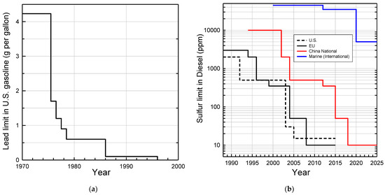
Figure 1. Reductions in regulatory limits for: (a) lead added to U.S. gasoline; (b) sulfur in diesel in the U.S., EU, China, and in marine fuel. The U.S. voluntary standard for lead from 1958 to 1975 was 4 cm³ tetra-ethyl lead per gallon which equates to 4.23 g Pb per gallon. The industry average use was approximately 2.4 g Pb per gallon in the 1950s and 1960s. The EPA required the availability of one grade of unleaded gasoline by 1974 to protect catalytic converters introduced in 1975. Limits from 1975 to 1986 were specified based on “pool averaging” allowing refiners to average over all grades of gasoline, including unleaded. In 1986 pool averaging was discontinued and the limit referred to leaded gasoline. The addition of lead to U.S. gasoline for road vehicles was banned in 1996 (https://www.epa.gov/history/epa-history-lead, accessed on 31 January 2022). Sulfur data were taken from https://www.transportpolicy.net/topic/fuels/, accessed on 31 January 2022.

4. Trends in Vehicle Emissions

Driven by increasingly stringent emission regulations, the combined effect of improvements in engine design, fuel systems, catalytic emission control systems, sensor technology, and electronic engine control systems, and evolving fuel formulations has led to spectacular decreases in vehicle emissions.

The University of Denver has conducted on-road optical remote sensing measurements of vehicle emissions over 30 years in Los Angeles [29] and over 20 years in Chicago [30]. The remote sensing technique measures the ratios of CO, HC, NO, SO₂, NH₃, and NO₂ to CO₂ in the exhaust plumes of individual vehicles as they pass by the monitoring equipment. A video camera captures the vehicle license plate information which can be used to determine the model year of the vehicle. The exhaust concentration ratios are converted into fuel-based emission factors (g pollutant emitted per kg fuel combusted) in the motor vehicle exhaust. Figure 2 shows CO and NO emissions as a function of the vehicle model year measured in Los Angeles in 1989, 1991, and 2018 and in Chicago in 2000 and 2020. Data for 1957–1962, 1963–1967, and 1968–1971 model year cars representative of the U.S. on-road fleet obtained in a laboratory study using the Federal Test Procedure driving cycle conducted in 1973 [31] are also shown in Figure 2. The systematic difference between the filled and open symbols in Figure 2b reflects the deterioration of the emission performance over the life of the vehicles (e.g., MY 2000 vehicles were less than a year old in the 2000 study but were about 20 years old in the 2020 study). The data in Figure 2 show the dramatic progress made in reduction of tailpipe emissions over the past 60 years. Remote measurements can be used to identify high emitting vehicles in the fleet for inspection and maintenance.

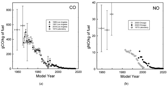
Figure 2. Emissions of CO (a) and NO (b) as a function of vehicle model year measured during on-road measurements conducted by Stedman, Bishop, and the research group at the University of Denver in Los Angeles and Chicago in 1989, 1991, 2000, 2018, and 2020 and in laboratory measurements by Fegraus et al. in 1973.

Measurements of emissions from uncontrolled vehicles prior to 1960 are limited. Hoekman and Westand [18] reviewed vehicle emission measurements in the 1940s–1950s. Based on dynamometer studies, the Los Angeles County Air Pollution Control District estimated daily automobile emissions within Los Angeles County in 1951 of 127 million ft³ CO, 132 tons NO_x, and 875 tons hydrocarbons, which equate to emission factors of 410 g CO/kg fuel, 11 g NO/kg fuel, and 70 g HC/kg fuel [32]. Real-world vehicle emission measurements were conducted in 1951 at the Stanford Research Institute in Pasadena, California. Four automobiles were studied: 2 from 1940–1941 and 2 from 1950–1951 [33]. The measurements involved towing a trailer behind the vehicles with grab samples taken from the exhaust for mass spectrometric chemical analysis. The work was expanded to include ten automobiles (5 each from 1940–1941 and 1950–1951) and it was estimated that 1016 tons of hydrocarbons (approximately 85 g/kg fuel) were emitted in the exhaust of the 1951–1952 fleet in Los Angeles [34]. The Los Angeles County Air Pollution Control District estimated daily automobile emissions within Los Angeles County in 1958 as 8850 tons CO, 1100 tons hydrocarbons, and 345 tons NO_x, which equate to emission factors of 480 g CO/kg fuel, 19 g NO/kg fuel, and 60 g HC/kg fuel [35]. Emission factors for uncontrolled (i.e., pre-1960) automobile exhaust were estimated by the U.S. Department of Health, Education, and Welfare to be 2300 lbs CO, 113 lbs NO_x, and 200 lbs HC per 1000 gallons of gasoline which equate to 365 g CO/kg fuel, 18 g NO/kg fuel, and 32 g HC/kg fuel [36]. Results from the four studies above are broadly consistent and taking an average gives emission factors of 420 g CO/kg fuel, 16 g NO/kg fuel, and 62 g HC/kg fuel from uncontrolled vehicles in the 1940s–1950s. Measurements reported in 1971 of a 1911 Model T Ford gave 120 g/mile CO, 2 g/mile NO_x, and 8 g/mile HC [37] which, assuming a fuel economy of 17 miles per gallon, equate to emission factors of 700 g CO/kg fuel, 12 g NO/kg fuel, and 50 g HC/kg fuel which are similar to those from unregulated vehicles in the 1940s and 1950s.

In addition to CO, HCs, NOx, and PM, the EPA and CARB track the emissions of gas-phase air toxics such as formaldehyde, acetaldehyde, acrolein, benzene, and 1,3-butadiene. Researchers at the University of California, Riverside reviewed the historical progress in reducing the emissions of air toxics from vehicles [38]. Figure 3a shows the emissions measured in the laboratory using the Federal Test Procedure for 410 light-duty gasoline vehicles showing the progress as successively more sophisticated emission control systems were added from the model year 1970 to 2000. As illustrated in Figure 3a, the introduction of emission control technology led to an approximately 100-fold reduction in the emissions of air toxins. This is approximately the same magnitude as the decrease in the emissions of total organic gases [38] indicating high effectiveness of the emission control systems across a wide range of organic compounds.

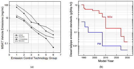
Figure 3. (a) Emissions of formaldehyde, acetaldehyde, 1,3-butadiene, and benzene from gasoline light-duty vehicles as increasingly sophisticated emission control technology was added over the vehicle model years 1970–2000. The technology groups are: (1) non-catalyst, (2) oxidation catalyst, (3) three-way catalysts, (4) transitional—low emission vehicles, (5) low emission (LEVs), and (6) ultra-low emission vehicles (ULEVs). (b) Evolution of emissions standards for NO_x and PM for heavy-diesel vehicles (updated from [39]).

Increasingly stringent NO_x and PM emission standards for diesel vehicles (Figure 3b) set by U.S. EPA in the 1980s and 1990s were met largely using increasingly advanced fuel injection systems, turbochargers, and exhaust gas recirculation. DOCs and catalyzed DPFs were added to meet the order of magnitude increase in PM emission standard stringency in 2007. Urea SCR catalysts were added to meet the new NO_x standard in 2010. A typical modern heavy-duty diesel emission control system now consists of, in order, a fuel injector upstream of the DOC (to assist DPF regeneration), DOC, DPF, urea injector, SCR, and finally an ammonia oxidation catalyst. Khalek et al. [40] conducted a comprehensive investigation of regulated and unregulated emissions from model year 2010 emissions compliant heavy-duty engines and reported reductions of PM, CO, NMHC, and NO_x of 99%, 97%, >99%, and 98%, respectively, relative to the 1998 standard. Unregulated emissions such as single-ring aromatics, polycyclic aromatic hydrocarbons (PAH), and nitro-PAH were reduced by 90%, 99%, and >99%, respectively.

While the data in Figure 2 and Figure 3 show that emissions on a per-vehicle per-mile basis have decreased it is important to recognize that the number of vehicles and the number of miles they are driven have increased. In the U.S., the vehicle miles travelled tripled between 1970 and 2019 [41]. The number of registered passenger cars in the EU grew about 66% from 1990–2019 and passenger car travel (passenger km) increased 30% from 1995–2019 [42]. Assessments of the impacts of vehicle emissions need to account for a number of factors including the distribution of ages of vehicles on the road, the number of miles and the manner in which they are driven, and emissions from tailpipe and non-tailpipe sources (e.g., evaporative emissions, brake-wear, and tire-wear). Figure 4 shows the absolute inventory of CO, NO_x, and HC emissions from the on-road fleet in the U.S. [43] and Europe (EU-28) [44] accounting for these factors. As seen from Figure 4, despite increased vehicle mileage, total highway vehicle (light-duty, heavy-duty, and commercial vehicle and motorcycle) CO, NO_x, and volatile organic compound (VOC) emissions in the U.S. and EU have decreased by 60–80% since 1990.

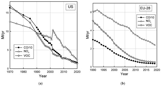
Figure 4. Total highway vehicle emissions in (a) the U.S. and (b) the EU-28, updated from Wallington et al. [45] see text for details.

Limits or bans on internal combustion engine vehicles (ICEV) are being considered in major cities and in some countries. California has a target stating that 100% of in-state sales of new passenger cars and trucks will be “zero-emission” by 2035. Zero-emission vehicles (ZEVs) are defined by the CARB as producing no emissions from the onboard source of power. The only technologies that meet this definition today are battery-electric vehicles and hydrogen fuel cell electric vehicles. Battery electric vehicles (BEVs) are being introduced at scale into the market. While BEVs do not have tailpipe emissions and hence have decreased local emissions, there are emissions associated with the generation of electricity that need to be considered on a regional scale. Table 1 shows emissions of criteria pollutants from BEVs running on U.S. average grid electricity compared with the best-in-class (lowest criteria emissions) U.S. ICEV, the U.S. average on-road fleet, typical Euro 6 gasoline direct injection (DI) ICEV real driving emissions (RDE), and the EU passenger car and the U.S. LDV standards updated from Winkler et al. [46]. The Euro 6 gasoline direct injection (DI) ICEV real driving emissions (RDE) reported by Winkler et al. [46] in 2018 are generally consistent with results published by the EU Joint Research Center in 2019 [47]. The best-in-class vehicle in the 2021 annual U.S. certification data is the Hyundai Sonata Hybrid [48]. The 2020 fleet average was taken from the remote sensing report of Bishop ([30]) with g/kg fuel emissions converted to mg/km using a fleet average 22.2 mpg [49]. The BEV emissions were calculated using a best-in-class efficiency (Tesla Model 3) of 0.24 kWh/mile and 2014–2019 grid emissions from the e-GRID database as discussed elsewhere [46]. Ranges for tire and brake wear emissions are from recent literature [50,51,52]. The best-in-class ICEV has about one order of magnitude lower tailpipe PM2.5 and HC and about two orders of magnitude lower NO_x emissions than a BEV powered by U.S. average grid electricity, while the 2020 on-road fleet average ICEV emissions are similar to those of this BEV. BEV emissions will decrease significantly by 2030 as the grid mix becomes cleaner. Finally, with the dramatically decreased vehicle tailpipe PM emissions there is increasing recognition of the increase in the relative contribution of non-tailpipe emissions such as brake and tire wear. As seen in Table 1, brake and tire wear is now a larger source of PM emissions than tailpipe emissions.

Table 1. Comparison of U.S. and EU vehicle emission standards (mg/km) with emissions from selected gasoline light-duty ICE vehicles and BEVs, and non-exhaust brake wear and tire wear emissions (updated from Winkler et al. [46] and Wallington et al. [45]).

	PM2.5	HC + NOx	NOx	SO2	CO
Vehicle Standards (test cycle)
U.S. Tier 3	2	36		0.6	1057
Euro 6 (gasoline)	0.3		60		1000
Euro 6 (diesel)	0.3 a	170	80		500
U.S. ICE
2021 Best-in-class (test cycle)	0.50	3.6	0.5		50
2020 Fleet average (on-road)		81	22		229
EU ICE
Average Euro 6 gasoline DI ICEV (RDE)	0.2–0.4		12–20		17–100
Most Efficient U.S. 2021 BEV
BEV-2014 U.S. elec. grid	6	67	66	116
BEV-2016 U.S. elec. grid	6	52	51	56
BEV-2019 U.S. elec. grid			42	39
BEV-2019 CA b elec. grid			25	2
BEV-2030 U.S. elec. grid			17	15
Tire and Brake Wear	PM2.5	PM10
Tire wear	5–7	5–10
Brake wear	1–5	1–20

^a Based on particle number standard of 6 × 10¹¹ #/km; 2 × 10¹² #/km is equivalent to ~1 mg/km. PM mass standard is 4.5 mg/km. ^b California; Notes: BEV emissions, best-in-class, 2020 Fleet Average, Tire and Brake Wear emissions were updated. The 2019 CA and U.S. electric grids were added; Creative Commons License: https://creativecommons.org/licenses/by/4.0/, accessed on 31 January 2022.

5. Trends in Air Quality

As the result of decreased emissions from mobile and stationary sources, the air quality in U.S. cities has improved substantially. Taking Los Angeles as an example, Figure 5a shows the decrease by a factor of approximately 10–100 in the concentrations of CO and volatile organic compounds and the decrease by a factor of approximately 5 in peak ozone levels (Figure 5b) over the past 50–60 years.

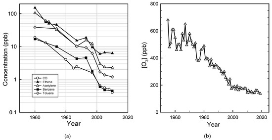
Figure 5. Progress in ambient air quality in the Los Angeles area: (a) CO and volatile organic compound concentrations 1960–2010 (data are from Warneke et al. [54]); (b) peak ozone levels (1955–1972 data are from the South Coast Air Quality Management District [55], 1973–2019 data are from the California Air Resources Board [56]).

Looking more broadly across cities in the U.S., Figure 6 shows trends in ambient air concentrations of key air pollutants in U.S. cities as measured by the U.S. EPA [53]. From 1980 to 2020 the national average levels of CO (annual 2nd maximum 8-h average), Pb (annual maximum 3-month average), NO₂ (annual 98th percentile of daily maximum 1-h average), O₃ (annual 4th highest 8-hr average), SO₂ (annual 99th percentile of daily maximum 1-h average) have decreased by 81%, 98%, 64%, 33%, and 94%, respectively [52]. PM2.5 (seasonally-weighted annual average) levels fell by 41% from 2000 to 2020. PM10 (annual 2nd maximum 24-h average) levels fell by 26% from 1990 to 2020. The dramatic progress in air quality shown in Figure 6 is even more remarkable considering the major increase in population (60% increase) and economic activity (GDP up by a factor of 3) over the past 50 years in the U.S.

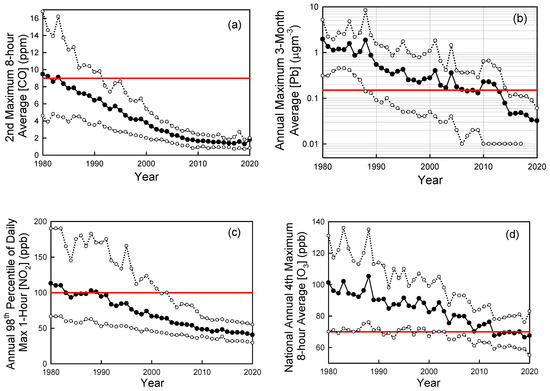
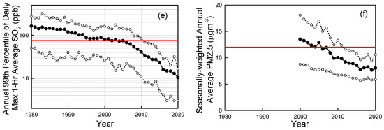
Figure 6. Trends in CO (a), lead (Pb) (b), NO₂ (c), ozone (d), SO₂ (e), and PM2.5 (f) in ambient urban air updated from Wallington et al. [45]. Solid symbols are averages, open symbols are 10th and 90th percentiles. The red horizontal lines are the primary National Ambient Air Quality Standards (NAAQS). Data were taken from the EPA Air Trends site [53] accessed in 2022 and 2019.

National Ambient Air Quality Standards (NAAQS) are set to protect public health and the environment. There are primary and secondary NAAQS. Primary standards (horizontal dashed lines in Figure 6) protect public health, including sensitive populations such as asthmatics, children, and the elderly. Secondary standards protect public welfare including damage to animals, crops, and buildings. As seen in Figure 6, with the exception of ozone, ambient pollution levels have fallen generally well below the NAAQS. Decreases in levels of CO, lead, and SO₂ have been particularly impressive with current levels in ambient air (shown in Figure 6a,b,e) now much lower than the NAAQS (note log scale in Figure 6b,e).

Ozone is formed in a complex series of reactions in the atmosphere, and its local concentration is a non-linear function of local, regional-, and hemispheric emissions of VOCs and NO_x. There is also a significant natural background of ozone of approximately 20–50 ppb depending on location and season [57]. These factors greatly complicate efforts to control ozone levels. While there has been major progress (see Figure 5b), elevated ozone levels are still an issue in many U.S. cities (see Figure 6d) and more work is needed to reduce emissions of the ozone precursors NO_x and VOCs.

PM2.5 levels have decreased to well below the 12 mg m⁻³ NAAQS in most U.S. locations (see Figure 6f). However, recent epidemiological research suggests that there may be adverse health impacts associated to exposure to levels below the current standard [58]. It is unclear whether the association revealed in this epidemiological study reflects a causal link between exposure and health impacts, or whether factors such as exposure to noise or access to green space (not considered in the study) confound the results. The WHO recently revised its annual PM2.5 air quality guideline from 10 to 5 mg m⁻³ [59]. Further work is needed to better understand the health impacts of exposure to low levels of PM2.5 and whether the current NAAQS is adequate.

NO₂ levels in ambient air have fallen by a factor of 2–3 to levels that are well below the daily maximum 1-h NAAQS of 100 ppb (Figure 6c). In addition to the 1-h standard established in 2010, there is an annual average standard of 53 ppb set in 1971. Typical annual average NO₂ concentrations are approximately 10 ppb; a factor of 5 below the standard. The EPA reviewed the NO₂ standards in 2018 and decided that no changes were needed. The EU has an annual average limit value of 40 μg m⁻³ (21 ppb) which is a factor of 2.5 times lower than the 53 ppb U.S. standard. The WHO annual air quality guideline for NO₂ is 10 μg m⁻³ [59]. Results are mixed from recent large-scale epidemiological studies on whether there are health impacts associated with exposure to NO₂ levels below the standards in the U.S. and EU. A study in the U.S. did not find any statistically significant association [58] while a similar study in Europe did find a significant association [60]. As with PM2.5, further work is needed to better understand the health impacts of exposure to low levels of NO₂. As discussed in the introduction, NO₂ and NO are rapidly interconverted in the sunlit atmosphere, and it is convenient to refer to their sum (NO + NO₂) as NO_x. Trends of decreased NO_x and NO₂ levels in ambient air are similar and closely match those of decreased road-vehicle NO_x emissions in emission inventories [61].

6. Pollutant Levels in Vehicle Exhaust Compared to NAAQS

Given the impressive strides made in reducing vehicle tailpipe emissions, it is of interest to ask the question “how do pollutant levels in the undiluted raw exhaust from a vehicle representative of the current on-road fleet compare to the current national ambient air quality standards (NAAQS)?” To answer this question, we use the 2020 U.S. on-road fleet average g/km ICE vehicle CO and NO_x emissions of 229 mg/km (0.37 g/mile) and 22 mg/km (35 mg/mile) from Table 1 and assume that vehicle PM emissions are at the Tier 3 Bin 30 certification level of 1.9 mg/km (0.003 g/mile). We then make three additional assumptions. First, the vehicle operates on E10 fuel at a stoichiometric air-fuel ratio of 14.05 with a fuel economy of 30 mpg. Second, NO_x emissions can be equated with NO₂ emissions, and PM emissions can be equated with PM2.5. Third, vehicle exhaust is cooled to ambient temperature, the gasoline exhaust density at ambient conditions is 1.217 kg m⁻³, and the exhaust has a molar mass of 28.8 g mol⁻¹.

Table 2 shows the results of the calculations. The final column in Table 2 shows the ratios of the concentrations of CO, NO₂, and PM2.5 in the raw exhaust compared to the current NAAQS. The approximate nature of these estimates should be noted. Emissions will vary from vehicle to vehicle and are not constant over a drive cycle; there will be times when the emissions are higher (particularly at engine start when the engine and after-treatment system are cold) and times when the emissions are lower (when the engine is warmed up and at light load). We do not consider the conversion of gas-phase emissions of HC and NOx into secondary aerosol formation. Nevertheless, the values in Table 2 provide the order of magnitude comparisons of how average pollutant concentrations in undiluted exhaust compare with the NAAQS. As seen in Table 2 the levels of CO, NO₂, and PM in the raw exhaust are of the order of 10 s–100 s of times higher than the NAAQS. Clearly, even modern vehicle exhaust has the potential to contribute significantly to the deterioration of urban air quality. However, it should be noted that vehicle exhaust is rapidly diluted by ambient air. Under typical driving conditions, turbulent mixing with ambient air leads to dilution of the exhaust by approximately a factor of 1000–10,000 within the first second [62].

Table 2. Pollutant concentrations in raw undiluted exhaust typical of the on-road 2020 fleet compared to NAAQS (ppm and ppb units are on a volume basis).

Pollutant	Exhaust (g/mi)	Exhaust	NAAQS	Exhaust/NAAQS
CO	0.37	260 ppm	9 ppm	29
NO2	0.035	15 ppm	100 ppb	150
PM2.5	0.003	2600 µg m−3	12 µg m−3	220

7. Discussion

We have provided an overview of 60 years of progress in reducing vehicle emissions and improvements in air quality in the U.S. As shown in Figure 2, NO_x and CO emissions were approximately 25 g/kg fuel and 500 g/kg for a typical light-duty vehicle in 1960. Using the 1960 average fuel economy of 14 mpg [48] gives NO_x and CO emissions of 3.2 and 64 g/km. The average emissions from the on-road 2020 fleet (see Table 2) of 22 mg/km NO_x and 229 mg/km CO are factors 145 and 280 times lower than those in 1960. Put another way there has been an approximately 99.3% and 99.6% reduction in the per vehicle per km emissions of NO_x and CO. Traffic volumes and the number of vehicles on the road have increased, leading to vehicle miles traveled in the U.S. increasing by a factor of 4.5 from 1960 to 2019 (from 0.72 to 3.26 trillion [48]). However, despite increased vehicle numbers and vehicle miles traveled, the absolute emissions have decreased substantially (see Figure 4).

As a result of decreased emissions from vehicles and stationary sources, the air quality in U.S. cities has improved dramatically. The peak level of ozone in Los Angeles smog has decreased by a factor of approximately 5 since the 1950s (see Figure 5b). The average concentrations of CO, lead, NO₂, ozone, SO₂, and PM2.5 measured at urban sites were all above the current national air quality standards 20–40 years ago but now are all below the standards (see Figure 6).

With the large decrease in vehicle emissions, the relative importance of other sources of emissions in urban areas has increased. The use of volatile chemical products, such as personal care products and cleaning agents, is now estimated to account for 50–80% of emissions, reactivity, and aerosol-forming potential of urban anthropogenic VOCs [63,64,65]. Food preparation in restaurants is a major source of PM in ambient air in urban areas and can dominate air pollution on a neighborhood scale [66]. With the drop in emissions from vehicles, biogenic emissions are now a major source of secondary organic aerosol in Los Angeles [67]. We have witnessed a profound change in the absolute and relative importance of vehicle emissions of VOCs. VOC emissions from highway vehicles in the U.S. have decreased by a factor of 12 (16.9 to 1.38 Mt yr⁻¹, see Figure 4a) from 1970 to 2020. Emissions of VOCs from vehicles are now at such a low level that in many areas they are less important than emissions from other anthropogenic sources.

Looking to the future it is clear that the trends of decreasing vehicle emissions shown in Figure 4 will continue for at least the next 10–20 years, primarily because new vehicles entering the fleet are dramatically cleaner than old vehicles retiring from the fleet. Hence, even if future emission standards were not tightened, and even if electric vehicles did not come into the fleet, the downward emission trend would continue. Nonetheless, it is likely that future emission standards will be tightened. Moreover, and more significantly, most major vehicle manufacturers have announced aggressive electrification goals and the Biden administration has announced a target of 50% electric share of new vehicle sales in 2030, with similar targets being pursued in other countries. A major increase in the number of BEVs will accelerate the decline in vehicle emissions in urban areas.

We have seen tremendous progress in reducing vehicle emissions and a yet lower emissions future lies ahead.

References

- Finlayson–Pitts, B.J.; Pitts, J.N.J. Chemistry of the Upper and Lower Atmosphere; Academic Press: San Diego, CA, USA, 2000; pp. 349–360. [Google Scholar]
- Haagen-Smit, A.J. Chemistry and Physiology of Los Angeles Smog. Ind. Eng. Chem. 1952, 44, 1342–1346. [Google Scholar] [CrossRef]
- Blacet, F.E. Photochemistry in the Lower Atmosphere. Ind. Eng. Chem. 1952, 44, 1339–1342. [Google Scholar] [CrossRef]
- Haagen-Smit, A.J.; Bradley, C.E.; Fox, M.M. Ozone Formation in Photochemical Oxidation of Organic Substances. Ind. Eng. Chem. 1953, 45, 2086–2089. [Google Scholar] [CrossRef]
- Haagen-Smit, A.J.; Fox, M.M. Automobile Exhaust and Ozone Formation. SAE Trans. 1955, 53, 575–580. [Google Scholar]
- Renzetti, N.A. Ozone in the Los Angeles Atmosphere. J. Chem. Phys. 1956, 24, 909–910. [Google Scholar] [CrossRef]
- Rogers, L.H. Report on Photochemical Smog. J. Chem. Educ. 1958, 35, 310–313. [Google Scholar] [CrossRef]
- Stephens, E.R.; Scott, W.E.; Hanst, P.L.; Doerr, R.C. Recent Developments in the Study of the Organic Chemistry of the Atmosphere. J. Air Pollut. Control Assoc. 1956, 6, 159–165. [Google Scholar] [CrossRef]
- Stephens, E.R. Absorptivities for Infrared Determination of Peroxyacyl Nitrates. Anal. Chem. 1964, 36, 928–929. [Google Scholar] [CrossRef]
- Leighton, P.J. Photochemistry of Air Pollution; Academic Press: San Diego, CA, USA, 1961; p. 312. [Google Scholar]
- Altshuller, A.P.; Bufalini, J.J. Photochemical Aspects of Air Pollution. Review. Environ. Sci. Technol. 1971, 5, 39–64. [Google Scholar] [CrossRef]
- Weinstock, B. Carbon Monoxide: Residence Time in the Atmosphere. Science 1969, 166, 224–225. [Google Scholar] [CrossRef] [PubMed][Green Version]
- Dixon-Lewis, G.; Wilson, W.E.; Westenberg, A.A. Studies of Hydroxyl Radical Kinetics by Quantitative ESR. J. Chem. Phys. 1966, 44, 2877–2884. [Google Scholar] [CrossRef]
- Levy, H., II. Normal Atmosphere: Large Radical and Formaldehyde Concentrations Predicted. Science 1971, 173, 141–143. [Google Scholar] [CrossRef]
- Logan, J.A.; Prather, M.J.; Wofsy, S.C.; McElroy, M.B. Tropospheric chemistry: A Global Perspective. J. Geophys. Res. Earth Surf. 1981, 86, 7210–7254. [Google Scholar] [CrossRef]
- California Air Resources Board. 2022. Available online: https://ww2.arb.ca.gov/about/history (accessed on 12 January 2022).
- Wallington, T.J.; Kaiser, E.W.; Farrell, J.T. Automotive Fuels and Internal Combustion Engines: A Chemical Perspective. Chem. Soc. Rev. 2006, 35, 335–347. [Google Scholar] [CrossRef]
- Hoekman, S.K.; Welstand, J.S. Vehicle Emissions and Air Quality: The Early Years (1940s–1950s). Atmosphere 2021, 12, 1354. [Google Scholar] [CrossRef]
- U.S. Energy Information Agency. 2022. Available online: https://www.eia.gov/energyexplained/use-of-energy/transportation.php (accessed on 12 January 2022).
- Haywood, J.B. Internal Combustion Engine Fundamentals, 2nd ed.; Mc Graw Hill: New York, NY, USA, 2018. [Google Scholar]
- Environmental Protection Agency. The 2021 EPA Automotive Trends Report, EPA-420-R-21-023; Environmental Protection Agency: Washington, DC, USA.
- Zeldovich, J. The Oxidation of Nitrogen in Combustion and Explosions. Acta Physicochim. URSS 1946, 21, 577–628. [Google Scholar]
- Jensen, D.A.; Grant, E.P. Status of Control of Motor Vehicle Emissions in California. J. Air Pollut. Control Assoc. 1964, 14, 483–522. [Google Scholar] [CrossRef]
- Cheng, W.K.; Hamrin, D.; Heywood, J.B.; Hochgreb, S.; Min, K.; Norris, M. An Overview of Hydrocarbon Emissions Mechanisms in Spark-Ignition Engines. SAE Tech. Pap. Ser. 1993, 932708. [Google Scholar]
- Frenkel, M. Deodorisation of Exhaust Gases in Motor Vehicles. J. Soc. Ind. Chem. 1909, 28, 692–693. [Google Scholar]
- Twigg, M.V. Catalytic Control of Emissions from Cars. Catal. Today 2011, 163, 33–41. [Google Scholar] [CrossRef]
- Nelson, P.F. Evaporative Hydrocarbon Emissions from a Large Vehicle Population. J. Air Pollu. Control Assos. 1981, 31, 1191–1193. [Google Scholar] [CrossRef]
- DieselNet Emission Standards. Available online: https://dieselnet.com/standards/us/ld_t3.php (accessed on 12 January 2022).
- Bishop, G.A. Three Decades of on-road Mobile Source Emissions Reductions in South Los Angeles. J. Air Waste Manag. Assos. 2021, 69, 967–976. [Google Scholar] [CrossRef]
- Bishop, G.A. On-Road Remote Sensing of Automobile Emissions in the Chicago Area: Fall 2020. CRC Report No. E-123, Coordinating Research Council. 2021. Available online: https://crcao.org/published-report/ (accessed on 21 September 2021).
- Fegraus, C.E.; Domke, C.J.; Marzen, J. Contribution of the Vehicle Population to Atmospheric Pollution; SAE International: Warrendale, PA, USA, 1975; p. 730530. [Google Scholar]
- Larson, G.P.; Fischer, G.I.; Hamming, W.J. Evaluating Sources of Air Pollution. Ind. Eng. Chem. 1953, 45, 1070–1074. [Google Scholar] [CrossRef]
- Magill, P.L.; Hutchison, D.H.; Stormes, J.M. Hydrocarbon Constituents of Automobile Exhaust Gases. In Proceedings of the Second National Air Pollution Symposium (Stanford Research Institute), Pasadena, CA, USA, 5–6 May 1952; pp. 71–83. [Google Scholar]
- Hutchison, D.H.; Holden, F.R. An Inventory of Automobile Gases. J. Air Pollut. Control Assoc. 1955, 5, 71–118. [Google Scholar] [CrossRef]
- Chass, R.L.; Tow, P.S.; Lunche, R.G.; Shaffer, N.R. Total Air Pollution Emissions in Los Angeles County. J. Air Pollut. Control Assoc. 1960, 10, 351–366. [Google Scholar] [CrossRef] [PubMed][Green Version]
- Duprey, R.L. Compilation of Air Pollutant Emission Factors; U. S. Department of Health, Education, and Welfare: Washington, DC, USA, 1968; Report 999-AP-42.
- Russell, G.A.; McGowan, J.G.; Ambs, L.A. Exhaust Emissions from a Model “A” Ford. Model A News 1971, 18, 20–21. [Google Scholar]
- Zhu, X.; Durbin, T.D.; Norbeck, J.M.; Cocker, D. Internal Combustion Engine (ICE) Air Toxic Emissions. Final Report CARB Contract 02-334A, California Air Resources Board; 2004. Available online: https://ww3.arb.ca.gov/research/single-project_ajax.php?row_id=60365 (accessed on 5 September 2019).
- Wallington, T.J.; Lambert, C.K.; Ruona, W.C. Diesel Vehicles and Sustainable Mobility in the U.S. Energy Policy 2013, 54, 47–53. [Google Scholar] [CrossRef]
- Khalek, I.A.; Blanks, M.G.; Merritt, P.M.; Zielinska, B. Regulated and Unregulated Emissions from Modern 2010 Emissions-compliant Heavy-duty Diesel Engines. J. Air. Waste Man. Assoc. 2015, 65, 987–1001. [Google Scholar] [CrossRef] [PubMed]
- U.S. Federal Highway Administration. Traffic Volume Trends. Available online: https://www.fhwa.dot.gov/policyinformation/travel_monitoring/tvt.cfm (accessed on 1 February 2022).
- European Union Transport in Figures: Statistical Pocketbook 2021. Available online: https://data.europa.eu/doi/10.2832/733836 (accessed on 21 February 2021).
- U.S. EPA. Air Pollutant Emissions Trends Data. Available online: https://www.epa.gov/air-emissions-inventories/air-pollutant-emissions-trends-data (accessed on 1 February 2022).
- European Environmental Agency, EEA. Air Pollutant Emissions Data Viewer (Gothenburg Protocol, LRTAP Convention 1990–2019). Available online: https://www.eea.europa.eu/data-and-maps/dashboards/air-pollutant-emissions-data-viewer-4 (accessed on 19 August 2021).
- Wallington, T.J.; Anderson, J.E.; He, X.; Ruona, W.C.; Shen, W.; Vogt, R.; Winkler, S.L. Light-duty Vehicle Emissions: An Automotive Perspective. EM Magazine, Air and Waste Water Management Association, April 2020. [Google Scholar]
- Winkler, S.L.; Anderson, J.E.; Garza, L.; Ruona, W.C.; Vogt, R.; Wallington, T.J. Vehicle Criteria Pollutant (PM, NOx, CO, HCs) Emissions: How Low Should We Go? Npj Clim. Atmospheric Sci. 2018, 1, 26. [Google Scholar] [CrossRef]
- Clairotte, M.; Valverde Morales, V.; Bonnel, P.; Gruening, C.; Pavlovic, J.; Manara, D.; Loos, R.; Giechaskiel, B.; Carriero, M.; Otura Garcia, M.; et al. Joint Research Centre 2019 Light-Duty Vehicles Emissions Testing, EUR 30482 EN; Publications Office of the European Union: Luxembourg, 2020; ISBN 978-92-76-26951-9. [CrossRef]
- United States Environmental Protection Agency. Compliance and Fuel Economy Data-Annual Certification Data for Vehicles, Engines, and Equipment. Available online: https://www.epa.gov/compliance-and-fuel-economy-data/annual-certification-data-vehicles-engines-and-equipment (accessed on 1 June 2021).
- Federal Highway Administration. Highway Statistics Series Publications. Available online: https://www.fhwa.dot.gov/policyinformation/statistics.cfm (accessed on 12 January 2022).
- OECD. Non-Exhaust Particulate Emissions from Road Transport; Organisation for Economic Co-Operation and Development (OECD): Paris, France, 2020.
- Harrison, R.M.; Allan, J.; Carruthers, D.; Heal, M.R.; Lewis, A.C.; Marner, B.; Murrells, T.; Williams, A. Non-exhaust Vehicle Emissions of Particulate Matter and VOC from Road Traffic: A Review. Atmos. Environ. 2021, 262, 118592. [Google Scholar] [CrossRef]
- Agudelo, C.; Vedula, R.T.; Collier, S.; Stanard, A. Brake Particulate Matter Emissions Measurements for Six Light-Duty Vehicles Using Inertia Dynamometer Testing. SAE Tech. Pap. Ser. 2020, 3, 994–1019. [Google Scholar] [CrossRef]
- U.S. EPA Air Trends. Available online: https://www.epa.gov/air-trends (accessed on 3 February 2022).
- Warneke, C.; De Gouw, J.A.; Holloway, J.S.; Peischl, J.; Ryerson, T.B.; Atlas, E.; Blake, D.; Trainer, M.; Parrish, D.D. Multiyear Trends in Volatile Organic Compounds in Los Angeles, California: Five Decades of Decreasing Emissions. J. Geophys. Res. Atmos. 2012, 117, D00V17. [Google Scholar] [CrossRef]
- South Coast Air Quality Management District, The Southland’s War on Smog: 50 Years of Progress on Clean Air. Available online: https://www.aqmd.gov/home/research/publications/50-years-of-progress (accessed on 1 March 2022).
- California Air Resources Board, Data Statistics Homepage. Available online: https://www.arb.ca.gov/adam (accessed on 2 February 2022).
- Calvert, J.G.; Orlando, J.J.; Stockwell, W.R.; Wallington, T.J. The Mechanisms of Reactions Influencing Atmospheric Ozone; Oxford University Press (OUP): Oxford, UK, 2015; pp. 16–30. [Google Scholar]
- Dominici, F.; Zanobetti, A.; Schwartz, J.; Braun, D.; Sabath, B.; Wu, X. Assessing Adverse Health Effects of Long-Term Exposure to Low Levels of Ambient Air Pollution: Implementation of Causal Inference Methods. Health Effects Institute Report 211. 2022. Available online: https://www.healtheffects.org/publications (accessed on 1 March 2022).
- World Health Organization. WHO Global Air Quality Guidelines; World Health Organization: Geneva, Switzerland, 2021; ISBN 978-92-4-003422-8. [Google Scholar]
- Brunekreef, B.; Strak, M.; Chen, J.; Anderson, Z.J.; Atkinson, R.; Bauwelinck, M. Mortality and Morbidity Effects of Long-term Exposure to Low-level PM2.5, BC, NO2, and O3: An Analysis of European Cohorts in the ELAPSE Project. Health Effects Institute Report 208. 2021. Available online: https://www.healtheffects.org/publications/research-reports (accessed on 1 March 2022).
- Yu, K.A.; McDonald, B.C.; Harley, R.A. Evaluation of Nitrogen Oxide Emission Inventories and Trends for On-Road Gasoline and Diesel Vehicles. Environ. Sci. Technol. 2021, 55, 6655–6664. [Google Scholar] [CrossRef] [PubMed]
- Men, Y.; Lai, Y.; Dong, S.; Du, X.; Liu, Y. Research on CO dispersion of a Vehicular Exhaust Plume using Lattice Boltzmann Method and Large Eddy Simulation. Transp. Res. Part D Transp. Environ. 2017, 52, 202–214. [Google Scholar] [CrossRef]
- McDonald, B.C.; de Gouw, J.A.; Gilman, J.B.; Jathar, S.H.; Akherati, A.; Cappa, C.D.; Jimenez, J.L.; Lee-Taylor, J.; Hayes, P.L.; McKeen, S.A.; et al. Volatile chemical products emerging as largest petrochemical source of urban organic emissions. Science 2018, 359, 760–764. [Google Scholar] [CrossRef] [PubMed]
- Coggon, M.M.; Gkatzelis, G.I.; McDonald, B.C.; Gilman, J.B.; Schwantes, R.H.; Abuhassan, N.; Aikin, K.C.; Arend, M.F.; Berkoff, T.A.; Brown, S.S.; et al. Volatile Chemical Product Emissions Enhance Ozone and Modulate Urban Chemistry. Proc. Natl. Acad. Sci. USA 2021, 118, e2026653118. [Google Scholar] [CrossRef]
- Gkatzelis, G.I.; Coggon, M.M.; McDonald, B.C.; Peischl, J.; Gilman, J.B.; Aikin, K.C.; Robinson, M.A.; Canonaco, F.; Prevot, A.S.H.; Trainer, M.; et al. Observations Confirm that Volatile Chemical Products Are a Major Source of Petrochemical Emissions in U.S. Cities. Environ. Sci. Technol. 2021, 55, 4332–4343. [Google Scholar] [CrossRef] [PubMed]
- Robinson, E.S.; Gu, P.; Ye, Q.; Li, H.Z.; Shah, R.U.; Apte, J.S.; Robinson, A.L.; Presto, A.A. Restaurant Impacts on Outdoor Air Quality: Elevated Organic Aerosol Mass from Restaurant Cooking with Neighborhood-Scale Plume Extents. Environ. Sci. Technol. 2018, 52, 9285–9294. [Google Scholar] [CrossRef] [PubMed]
- Nussbaumer, C.M.; Cohen, R.C. Impact of OA on the Temperature Dependence of PM2.5 in the Los Angeles Basin. Environ. Sci. Technol. 2021, 55, 3549–3558. [Google Scholar] [CrossRef] [PubMed]
Publisher’s Note: MDPI stays neutral with regard to jurisdictional claims in published maps and institutional affiliations. |
© 2022 by the authors. Licensee MDPI, Basel, Switzerland. This article is an open access article distributed under the terms and conditions of the Creative Commons Attribution (CC BY) license (https://creativecommons.org/licenses/by/4.0/).