Abstract
The intermittent nature of wind resources is challenging for their integration into the electrical system. The identification of weather systems and the accurate forecast of wind ramps can improve wind-energy management. In this study, extreme wind ramps were characterized at four different geographical sites in terms of duration, persistence, and weather system. Mid-latitude systems are the main cause of wind ramps in Mexico during winter. The associated ramps last around 3 h, but intense winds are sustained for up to 40 h. Storms cause extreme wind ramps in summer due to the downdraft contribution to the wind gust. Those events last about 1 to 3 h. Dynamic downscaling is computationally costly, and statistical techniques can improve wind forecasting. Evaluation of the North American Mesoscale Forecast System (NAM) operational model to simulate wind ramps and two bias-correction methods (simple bias and quantile mapping) was done for two selected sites. The statistical adjustment reduces the excess of no-ramps (≤|0.5| m/s) predicted by NAM compared to observed wind ramps. According to the contingency table-derived indices, the wind-ramp distribution correction with simple bias method or quantile mapping method improves the prediction of positive and negative ramps.
1. Introduction
Wind energy is an alternative electricity generation prospect, and can reduce carbon dioxide emissions into the atmosphere, unlike fossil fuels. The intermittent nature of this power source has prompted the development/refinement of wind forecasting systems. One aspect to consider when evaluating models is their ability to reproduce the high-frequency variations of the wind. These changes in the magnitude of the wind in periods ranging from minutes to hours are defined as ramps. Ramp events can represent a critical situation for energy systems, due to an energy imbalance and associated costs. There are several definitions of wind-power ramp [1,2], such as, for instance, a percentage of change of the rated power or as a specific value of power related to the size of the wind farm. Wind-power ramps obtained from wind farm records can originate from the management of the wind farm and are not necessarily associated with an atmospheric phenomenon [2]. Wind ramps reveal the presence of atmospheric phenomena such as cold fronts, hurricanes, storms, sea–land breezes, valley–mountain breezes, etc.
Wind-power ramps are challenging for power-system operators, as they must manage grid operations to optimize costs and avoid damage to the power grid or wind turbines. The prediction of wind ramps is useful for reducing the uncertainty of electricity generation. Wind-power operators need to anticipate the amplitude and timing of wind ramps for better integration into the power grid. With the planned growth of the wind-power share of the global electricity portfolio, wind ramps may become a critical issue. Intermittent and abrupt changes in wind speed pose a risk to grid stability, especially during periods of low generation when there is limited availability of reserve power [3]. Curtailment of wind ramps represents a loss of potential profits and a possible increase in energy prices [4]. Mismanagement of wind ramps can result in power outages. Recently, assessment of wind-ramp forecasting using NWP models has grown [2,3,5,6,7], in order to implement adequate management of wind farms and mitigate issues as grid instability and economic losses. Regions with wind-energy potential are usually located over complex terrain where the near-surface flow is difficult to simulate. As result, model improvements are necessary for better wind-speed and wind-ramp prediction. Forecast errors can be associated with initial conditions or with the description of physical processes in the models [7].
Improving numerical weather prediction (NWP) (see Table S1 in Supplementary Material for a list of abbreviations) models require relevant observational data for the assessment of NWP performance for wind energy. Observations of meteorological towers and LiDAR permit the evaluation of the horizontal and vertical distribution of the wind; the latter is particularly important to determine the wind speed at the height of the rotor layer, to avoid vertical wind interpolation. Projects such as the Wind Forecast Improvement Project (WFIP) [4] have been designed to improve the accuracy of short-term (0–6 h) wind-power forecasting. The WFIP used wind profile radars, sodars, several LiDARs, and surface flux stations, instrumented tall towers, and nacelle anemometers. A reduction (12–5% for forecast hours 1–12) in power root-mean-square error was achieved from the combination of improved numerical weather prediction models and the assimilation of new observations [8]. A reduction of errors can also be obtained through statistical correction or post-processing data. Post-processing is used to adjust the model bias to historical observational data [9]. Ensemble predictions of NWP are constructed under several initial conditions or several physical parameterizations, and the runs capture the inherent uncertainty in model outputs. An ensemble prediction of planetary boundary layer (PBL) parameterizations can be useful in wind forecast [10].
A short-range weather forecast is a key component for the improvement of decision-making under weather situational awareness. NWP forecasts especially for rapidly changing weather conditions require frequent updates. In response to that problem, the Rapid Update Cycle was created [11]. This was replaced by the Rapid Refresh Model (RAP) in 2012. RAP is used for various applications including aviation, severe weather, and energy [11]. The ability of the model for capturing severe weather conditions can help predict wind ramps related to storms.
Understanding the weather systems that generate wind ramps at specific locations can be helpful for designing a model configuration that reproduces adequately weather event characteristics. Middle-latitude systems are the main weather systems that produce large wind-speed changes in winter in Mexico [12]. However, a common issue in the prediction of wind ramps is their magnitude and timing.
On the other hand, predictability in summer is low because the systems that originate the ramps are mesoscale systems such as valley–mountain and sea–land breezes or Mesoscale Convective Systems [12]. Synoptic systems dominate the weather in winter and they can be forecasted days in advance with good accuracy. In summer, local effects such as the differential warming of hills and valleys or land and sea surfaces produce thermally driven circulations that dominate the weather. Soil moisture and atmospheric instability help the development of scattered showers and thunderstorms [13]. The triggers for a thunderstorm development can be difficult to determine some hours before its formation. The atmospheric processes involved in summer weather are complex, with an important interaction of topography. In mesoscale models, surface inhomogeneities resulting from a rough description of terrain and/or surface features generates an inadequate representation of the above-mentioned processes [13]. Mesoscale models can reproduce horizontal and vertical temperature and humidity with high accuracy, but they have problems modeling adequately shallow and deep convection, leading to misallocation of centers of convection activation [13].
The identification of the meteorological phenomena that produce wind ramps in a region provides information on the characteristics of the ramps and the necessary refinements in the physical configuration of the model. The focus of the study is to present some tools to improve wind-ramp forecast. Wind generation cannot be fully controlled, unlike to conventional power plants (thermal or hydropower plants). The assessment of extreme wind events and the underlying role of weather regimes in triggering these events is crucial. Characterization can permit an increase in the predictability of wind ramps in terms of the seasonality of weather systems generating these ramps and the persistence of intense winds. Additionally, the examination of post-processing statistical tools for adjusting NWP outputs to local conditions can improve wind-ramp prediction. Cold fronts account for most of the ramps in winter. As a typical synoptic event, they are predictable several days in advance. However, ramps associated with storm events can be difficult to accurately predict more than a couple of hours in advance. Better storm prediction (time, intensity, and location) can lead to improved wind-ramp prediction in summer. In this study, extreme wind ramps were characterized at four different geographical sites in terms of duration, persistence, and weather system. Additionally, the skill in predicting ramps of an operational forecast model available for Mexico, the North American Mesoscale Forecast System (NAM), is evaluated. The outputs are freely accessible and contain information since 2006; however, its use for wind energy purposes has been little explored.
Section 2 introduces the horizontal wind observational data from weather stations and masts used in this study and a brief description of the NAM model. Additionally, in this section the definition of wind ramps, indices for the verification of ramp events, and bias-correction methods applied to NAM outputs are presented. The weather systems generating wind ramps at four different geographical sites in Mexico are discussed in Section 3. Ramp verification is included in Section 3. Lastly, conclusions are presented in Section 4.
2. Materials and Methods
The observational wind data used in this study are from two weather stations of the National Meteorological Service and two masts from the National Institute of Electricity and Clean Energies (Figure 1). Location and record periods are indicated in Table 1. Weather stations measure 10-m wind speed and direction every 10 min. Meanwhile, wind masts report winds at 20 m in Francisco Villa (FCOV) and at 15 m in La Venta (LVEN) every 10 min.
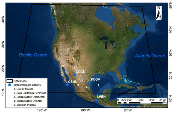
Figure 1.
Weather stations and masts (blue dots) used in the study and North American Forecast System (NAM) domain (black line). Cabo San Lucas (CSNL), Ciudad Cuauhtemoc (CDCU), Francisco Villa (FCOV), and La Venta (LVEN).

Table 1.
Description of measurement sites.
The mast installed in FCOV and LVEN measured the wind speed and the wind direction with NRG Maximum 40 cup anemometers and NRG 200P wind vane, respectively. The station monitored the variables every 2 s. It calculated and recorded speed average wind speed, wind gust, and wind direction every 10 min. The data-logger was a Campbell CR100. There are no specifications available of the equipment in Ciudad Cuauhtemoc (CDCU) and Cabo San Lucas (CSNL) weather stations. The observed hourly wind gust is the maximum 10 min wind gust observed for one hour.
2.1. NAM Model
NAM outputs were used to assess the ability of an operational model to predict wind ramps in Mexico. Bias-correction methods were applied to the model data for adjusting to the observed wind-ramp distribution. After this correction, NAM non-corrected and NAM-corrected data performance were assessed. CDCU and CSNL weather stations were used for wind-ramp evaluation because both have the longest and recent record periods (2010–2016). Additionally, both areas have wind-power potential, but wind farms have not been installed yet.
The NAM is one of the National Centers for Environmental Prediction’s (NCEP) major models for producing regional weather forecasts. NAM model forecasts were obtained from the National Oceanic and Atmospheric Administration’s (NOAA) National Centers for Environmental Information [14]. The NAM model has been running with a non-hydrostatic version of the Weather Research and Forecasting (WRF) model at its core since June 2006. The NAM is initialized with a 6-h data assimilation cycle with hourly analysis updates using the NCEP hybrid variational ensemble analysis for the 12 km parent domain (Figure 1). Wind-ramp verification was done using the 24-h NAM forecast initialized at 0000 UTC at 10 m height (the wind measurement height of weather station). The model uses hybrid sigma-pressure vertical coordinates, with 2 mb model top pressure and 60 vertical layers. Presently, NAM includes a full set of parameterizations for physical processes, including the Janjic-modified Betts–Miller convection and Mellor–Yamada–Janjic 2.5 scheme for turbulent exchange [15].
The NAM model runs multiple domains of weather forecasts over the North American continent at various horizontal resolutions [14]. High-resolution forecast windows are generated over fixed regions and are occasionally run to follow significant weather events, such as hurricanes. The NAM system is constantly tested and its configurations are modified to improve the quality of forecasts [16,17]. This system has been evaluated in terms of the process associated with convection initiation [18], which can influence the ability to predict wind ramps associated with storms. The NOAA Environmental Modeling Center looked extensively into the cause of noisy profiles of temperature and moisture in the presence of strong updrafts in NAMv3 [19], and ultimately developed a routine to stabilize all vertical layers above the boundary layer [20]. These changes were implemented in NAM version 4, which became operational in early 2017 [18]. The recent model improvements resulted in best simulation of storms tracks and outflows.
2.2. Wind-Power Spectra
The power spectra of wind-speed data were computed using the Fourier transform. For a clear representation of spectral peaks and valleys, the frequency-weighted form of the spectrum fS(f) is used [21,22,23]. We investigate the spectral structure for the four geographical sites. The construction of the wind-energy spectra was used to detect the relevant atmospheric phenomena in the production of wind ramps for each region. Atmospheric phenomena that significantly affect the region generate energy peaks in the spectrum, which are associated with a periodicity.
2.3. Wind Ramps
Probability density function (PDF) of the hourly wind-speed increments/decrements normalized by their standard deviation is constructed to analyze the differences among the four geographic locations, a similar procedure applied by DeMarco et al. [24].
For a time, increment (), the wind-speed ramp is defined as the difference between the wind speed at time + and the wind speed at the starting time (). The wind increment/decrement values are normalized by the standard deviation () [24].
The periods used for the calculation of observed PDFs are shown in Table 1. Observed PDFs of wind ramps show similar shape and heavier tails than Gaussian PDFs for different meteorological and topographical conditions (Figure S1 in Supplementary Material). Based on similar distributions for all four sites, we define extreme ramps as those exceeding four times the normalized deviation of the wind ramps ().
The verification of the ramp simulation with the NAM model was carried out by constructing indices derived from contingency tables. The ramp is considered positive (ramp-up) or negative (ramp-down) whether the wind speed increases or decreases over time. On verification, a ramp-up (down) event occurs when the wind-speed change is greater (less) than 0.5 m/s (−0.5 m/s) for one hour. A wind magnitude changing ≤|0.5| m/s is considered a no-ramp event.
2.4. Ramp Categorization
The weather circulation types are identified for every wind-ramp event. Winter wind ramps are mainly related to frontal system passages that cause prevailing intense wind from a persistent direction. Examining surface winds and the horizontal gradient of equivalent potential temperature at 700 mb using ERA5 shows the displacement of a cold front over the region. The verification of cold front position near the weather station was done using the MODIS-corrected reflectance images [25] for the day of the wind-ramp event. Cold front reports in newspapers were also consulted. Prefrontal and postfrontal wind intensification is usually experienced at weather station. In locations near the Gulf of Mexico, such as FCOV and LVEN masts, the interaction between topography and the high pressure systems associated with the cold front originates wind intensification events known as a “Norte” [26] or “Surada” [27].
Tropical cyclones and easterly tropical waves were associated with wind-ramp events examining trajectories of these systems in the NOAA Tropical Cyclone Reports [28].
A wind ramp is classified as related to storms when intensification of wind is observed in the weather station and precipitation occurs on the weather station or nearby. Additionally, cloud top height (AIRS2RET_NRT, [29]) and MODIS cloud top temperature [30] were analyzed to identify Mesoscale Convective Systems [31].
2.5. Downdrafts
Gustiness in horizontal winds near the surface is often associated with convection. Downdrafts possess vertical momentum which, on approaching the ground, is deflected to the horizontal [32,33]. Different convective gust models have been proposed [33]. Nakamura [32] considers that downdrafts are driven by three terms: the momentum of the parcel at the top of the downdraft, the latent heat-induced negative buoyancy of the air, and the precipitation loading effect. For quantifying the possible contribution of downdrafts in the wind ramps, we employed Nakamura-based scheme used by the Met Office [33].
where is the absolute temperature of the enviroment in K over depth in m, calculated under the assumption that for summer thunderstorms, the downdraught originates near the melting level for precipitation, given by the wet bulb temperature freezing level (). is the difference between the and in K. is the initial wind speed in m/s, is the maximum precipitation rate in mm/h and g is the acceleration due to gravity in m/s2.
2.6. Bias-Correction Methods
Bias adjustment is usually applied to model wind time series for reproducing similar statistical properties of observations [34], reducing systematic errors. They result from the inability of the NWP to reproduce all the relevant atmospheric processes and orographic interactions of flows. Additionally, bias originates from the initialization of data and model resolution [35]. In this study, two bias-adjustment methods have been applied to the 24-h NAM forecast of wind ramps: simple bias adjustment and quantile mapping adjustment.
The simple bias-correction scheme is summarized as:
Wind-ramp anomalies are calculated by subtracting the forecast mean to each forecast at a particular time . A new wind-ramp forecast is calculated by multiplying the NAM non-corrected forecast anomaly by the ratio of the standard deviation of the reference dataset (observations) () to the standard deviation of the NAM non-corrected wind-ramp forecast (). Finally, the mean of the reference data set is added to the anomaly.
Quantile mapping (QM) correction involves transforming the distribution functions of the modeled wind ramp into the observed ramp distribution using a mathematical function [34,36]. The method employs the PDFs of the reference dataset and the PDFs of the NAM forecasts in the reference period and then the empirical cumulative distribution function (CDF) is defined. A transfer function for correcting an independent forecast is defined as:
with a NAM-corrected forecast in a particular time, is the cumulative distribution function of NAM data and is the inverse cumulative distribution function of observation during the reference period. The QM method uses the quantile–quantile relationship to converge the simulated variables’ distribution function to the observed one. In cases where the data had missing values, the corresponding simulated values were omitted to obtain time series of equal length [37]. The years 2010–2015 were used as the reference period.
2.7. Contingency Table
Addressing the ability of NAM-corrected and NAM non-corrected is done through a contingency table [38]. The table summarizes the relationship between observed and forecasted wind ramps. A Hint or True Positive (TP) is the number of times a wind ramp is reproduced by the model, meanwhile the number of times a wind ramp is not forecasted is called a Miss or False Negative (FN). The events that are forecasted but not observed are called False Alarm or False Positive (FP). False Negative (FN) is the absence of wind ramps events correctly forecasted by the models. Indices for evaluating model performance in the detection of wind ramps are constructed with the elements of the contingency table. The following indices were used [38]:
Probability of detection (POD) measures the percentage of observed wind ramps (TP) that are correctly predicted by the model (TP + FN).
False Alarm Rate (FAR) is the percentage of forecasted events that were not observed.
Frequency bias (FBIAS) measures the ratio of forecasted ramp events to observed ramp events.
Critical success ratio (CSI) is the number of True Positive events between the forecasted events and the missed events (TP + FP + FN).
3. Results
3.1. Wind-Power Spectra
In this section, the analysis of long-term mean wind and turbulence data is discussed. Spectral peaks are evident in 3 × 10⁻⁸ Hz (1 year, see Figure S2), between 2 × 10⁻⁶ Hz and 3 × 10⁻⁶ Hz (3.9 to 5.7 days) and 1 × 10⁻⁵ Hz (1 day). Near-surface diurnal and sub-diurnal wind maxima decrease slightly with height. At frequencies higher than 8 × 10⁻⁵ Hz, the spectrum falls off −2/3 slope for the four sites (Figure 2). On the low-frequency side of the frequency-weighted spectrum, the yearly spectrum rises at f+1 from 10−7 to 10−6 Hz except for LVEN mast.
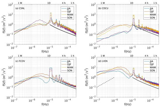
Figure 2.
Seasonal smoothed frequency-weighted spectra fS(f) of horizontal wind speed for (a) Cabo San Lucas (CSNL), (b) Ciudad Cuauhtemoc (CDCU), (c) Francisco Villa (FCOV), (d) La Venta (LVEN). The solid black line corresponds to the slope f−2/3. The dotted black line represents the f+1 slope. JJA: June–July–August (blue line); DJF: December–January–February (orange line); MAM: March–April–May (yellow line); SON: September–October–November (purple line).
Low-frequency events (~6 days) are more common in winter (yellow and orange lines in Figure 2) due to frontal systems over Mexico. Although these do not simultaneously affect the analyzed sites, they are the main middle latitudes synoptic modulators of winter weather. The effect of those systems is clearly observed at CDCU station (Figure 2b), during December–January–February (DJF) and March–April–May (MAM) as an increase in energy at the low-frequency side of the spectrum. Low-frequency maximum is associated with easterly waves during summer on southern Mexico. LVEN is the mast with the largest energy in the low-frequency side of the spectrum (Figure 2d), showing these synoptic phenomena are relevant for wind energy in the region. At CSNL station, the seasonal maximum of the spectrum in low-frequency events occurs in September–October–November (SON) (Figure 2a), due to tropical cyclone activity in the Pacific Ocean [39] and cold fronts passage over the region.
In summer, June–July–August (JJA) and starting in spring, local circulations intensify, as synoptic systems weaken, there is a decrease in energy associated with low-frequency events (Figure 2). The thermal differences caused by the heterogeneity of the surfaces produce local circulations with duration between 8 and 12 h, manifesting as daytime and hourly maxima in the spectrum that are more evident in the summer period. The spectral peak in 1 × 10⁻⁵ Hz of sea-breeze circulation is higher than the observed in middle latitudes. The appropriated prediction of these weather systems is important in spring and summer for a better representation of wind and wind ramps as mentioned by Pereyra-Castro et al. [12]. Near-surface diurnal and sub-diurnal wind maxima decrease slightly with height, they become less relevant as the wind rotor is far from the surface.
3.2. Characteristics of the Persistence of Wind Ramps
Extreme ramp events are caused by frontal systems during winter (Figure 3 and Figures S3–S5). Figure 3 shows the wind-ramp duration for extreme events. Every event started with a wind change exceeding four times the normalized deviation of wind ramps in one hour. After the initial increase in wind speed, it can continue going up, lasting from 2 to 4 h (ramp-up). After a wind-ramp event, the wind speed can be sustained within a given interval of intense wind-speed values, the duration is defined as persistence [40] (Figure S6). The regional orographic characteristics modify the persistence and intensity of the wind ramps. In LVEN mast, the low-level atmospheric flow is channeled into the Isthmus of Tehuantepec, where the winds associated with cold fronts generate ramps with an average duration of 6 h and intense winds lasting on average 40 h (Figure 3d). In FCOV mast, the ramps associated with cold fronts last 2.5 h and persist for 7 h on average. In the sites located in the northwest of Mexico, CDCU and CSNL, the intense events persist for 4 h (Figure 3a,b). One characteristic of cold fronts that needs to be highlighted is that a front that moves over the region of FCOV mast tends to generate intense winds in the Mexican Plateau (CFT), the effect of which can be seen in CDCU station. Similarly, a cold front over the Mexican Plateau will affect the intensity of the winds in the region of FCOV mast (CFP) and Baja California Peninsula.
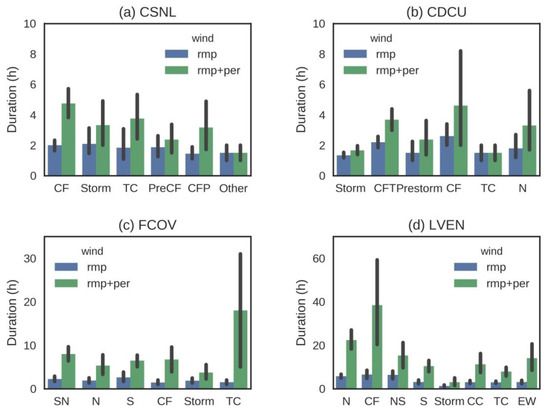
Figure 3.
Wind-ramp duration and associated intense winds at (a) CSNL, (b) CDCU, (c) FCOV, (d) LVEN. Weather systems: Cold front (CF), Tropical Cyclone (TC), Pre-Cold Front (PreCF), Nortes (N), Surada (S), Transition Surada to Norte (SN), Easterly wave (EW), Cyclonic Circulation (CC). Cold front over Plateau (CFP) and cold front over FCOV (CFT). Rmp means wind ramp and (Rmp + per) refers to the wind ramp and persistence of intense winds.
The anticyclonic circulations associated with the mid-latitude wave can cause northerly winds in the Gulf of Mexico > 30 m/s. These intense winds over the Gulf of Mexico are called Nortes. The average duration of the intense winds is 22 h in LVEN station and 6 h in FCOV mast with ramps of 4 to 5 h. Before a Norte, warm and intense southerly winds known as Suradas can be generated. These winds persist for up 10 h in LVEN mast and 8 h in FCOV mast. Some extreme ramps originate from Nortes to Surada or Surada to Nortes event transitions, which occur in 2 to 3 h periods, but strong winds persist for 10 to 14 h (Figure 3c).
In summer, the formation of Mesoscale Convective Systems (MCS) in some regions of Mexico generates extreme wind ramps of short duration; the winds intensify for 1 or 2 h and are sustained for another hour. Its duration does not vary with regional topographic characteristics. Strong winds associated with tropical cyclones and/or hurricanes can last for days, as seen in FCOV mast (Figure 3c). The persistence of ramp events depends on the proximity of the tropical cyclones to the study site, generating intense winds in periods of 1 to 8 h. At some stations during these events, the sensors do not register the wind, showing ramp events shorter than those observed.
3.3. Weather Conditions Generating Extreme Wind Ramps
Wind-ramp events observed during winter months are caused by the passage of cold fronts over Mexico; examples are shown in Figure 4. Surface winds are front position indicators at CDCU, CSNL, FCOV and LVEN. Westerly cold fronts tend to pass over CDCU station intensifying wind speed (Figure 4b). As they move eastward, they can also generate wind ramps at FCOV mast (Figure 4c) and LVEN mast. Cold fronts accelerate wind in the station, even if the cold front is not directly over the study point (Figure 4b). Wind-power variability can be dominated by synoptic phenomena for days changing the power production. The energy increase in the lower frequency side of the power spectrum during DEF and MAM (Figure 2). When passing over the Mexican Plateau, there is an intense westerly wind at CDCU station, generating ramps. At the same time, strong wind from the east or southeast is observed over the Gulf of Mexico (Figure 4b). These events generate wind ramps in the region of the FCOV station, when the wind is from the southeast. These events are similar to the weather patterns reported by Thomas et al. (2020) [41], they are common from January to May and they contribute significantly to extreme winds. The winter wind ramps in CDCU station and FCOV mast are related, the passage of a frontal system over CDCU station tends to generate ramps in FCOV mast and vice versa.
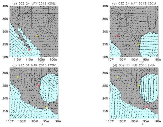
Figure 4.
Cold fronts affecting (a) CSNL, (b) CDCU, (c) FCOV and (d) LVEN. From ERA5 [42] surface wind for typical cold fronts causing wind ramp. Dots show weather stations location. Red dot indicates weather station or mast experiencing the wind ramp.
Wind-ramp events at CDCU and CSNL stations in summer are mainly caused by downdrafts of convective systems forming in Sierra Madre Occidental (Figure 5c) or around the region (Figure 5a). These events are usually short duration. Most intense precipitation occurs around the wind-ramp timing (lasting around 2 h). Trade winds intensification from the Gulf of Mexico also contributes to wind ramps over CDCU station and FCOV mast (Figure 5b). Trade winds carry moisture inland and can favor storm formation. Convective systems can also contribute to wind-ramp generation in LVEN mast.
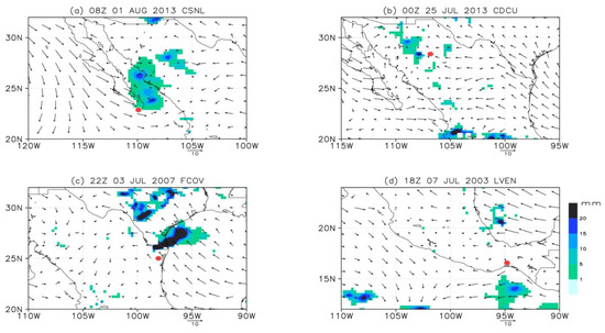
Figure 5.
Summer ramp-up events at (a) CSNL, (b) CDCU, (c) FCOV and (d) LVEN. Weather station location is indicated with a red circle. 3 h average ERA5 [42] surface wind speed and CMORPH [43] accumulated precipitation in mm (shaded) centered around the wind-ramp occurrence (weather station).
The meteogram illustrates the ramp event that occurred at CSNL station on 1 August 2013 (Figure 6). The storm formed over the Sierra Madre Occidental, then it moved eastward and reached the eastern coast of Baja California at 07:00 Z, where maximum precipitation presented according to CMORPH [43] data at 09:00 Z when the ramp occurs. According to the Nakamura storm gust formula [33] (Equation (2)), the gust in the core of the storm intensifies at 07:00 Z and it stands for 3 h and as the storm approaches the station, the ramp occurs. At 10:00 Z, the storm weakens considerably and a new core of maximum precipitation forms towards the north of Baja California Sur (Figure S7). At this new location, the precipitation is still intense but the distance between the station and the core of the storm is ~70 km (Figure S7). The wind ramp lasts around one hour due to the rapid dissipation of the storm. The storm trajectory forecasted by NAM model differs according to the initialization forecast hour (Figure S7), the displacement of the storm is more accurately predicted by the 06:00 Z NAM forecast initialization, near the ramp set up. On the other hand, the 00:00 Z NAM initialization predicts the movement of the storm parallel to the Sierra Madre Occidental.
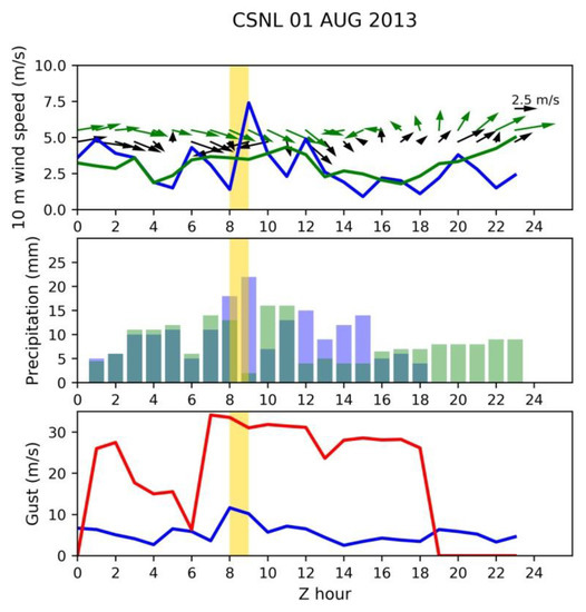
Figure 6.
Meteogram at CSNL station for a storm at 09:00 Z 01 August 2013. Wind-ramp timing is shaded in yellow. CMORPH [43] maximum precipitation in the center of the storm is in blue bars. Estimated wind gust in the storm is in red line and observed wind gust at CSNL is in blue. Forecasted wind speed, wind vector and precipitation are in green.
In the rest of the ramps shown in Figure 5, the time of occurrence of the ramp coincides with the moment when the storm is closest to the station, even when the precipitation is not the most intense observed during the day (Figures S8–S10). The calculated wind gusts (Equation (2)) due to convection are more intense than the ramps observed at the weather stations because the winds decrease due to the surface friction and the distance between the weather stations and the location where the storms are generated. The displacement of the storm can generate in some cases changes in the mean wind direction before the occurrence of the ramp.
3.4. Ramp Distribution Correction
Reanalysis data shows underestimation of high-frequency variability of wind [40]. Winds derived from simulations using mesoscale models also tend to be underestimated due to the spatial and temporal resolutions [44]. The smoothing effect conducts to the overestimation of weak ramp events in comparison to the observed ramps [45]. For this reason, it is necessary to adjust the simulated wind-ramp distribution to the observed distribution. The adjustment is done through simple bias and quantile mapping methods. The statistical corrections fit the predicted ramp distribution fairly well with respect to the observed distribution (Figure 7). Furthermore, to assess the correction effects on ramp forecasting, we use indices derived from contingency tables to compare the onset time of observed and forecast wind ramps. Both methods, as will be seen later, enhance POD index, improving wind-ramp forecasting.
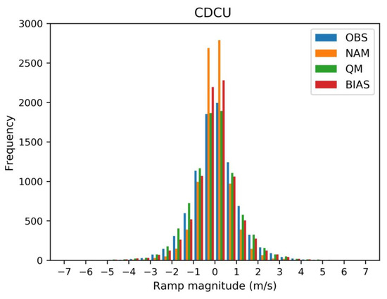
Figure 7.
Wind-ramp distribution for CDCU observations (blue bar), NAM (orange bar), Quantile mapping correction (QM) (green bar) and Simple bias correction (red bar).
A positive (negative) ramp is an increase (decrease) in wind speed for one hour. The ramp is correctly forecasted when an increment (decrement) in wind-speed change in 1 h is presented in the model wind speed for the same local hour of observation, this event is known as TP (Figure S11). A positive (negative) ramp produced by the model but not observed is a FP (Figure S11). Observed wind-speed changes that show an increment (decrement), but are not predicted are known FN (Figure S11). The effect of relaxing the time threshold was not tested in this study, in those cases a more sophisticated metric that incorporates phase, duration, and amplitude errors is discussed in Bianco et al. [5].
The ramps were grouped into no-ramps ≤|0.5| m/s, positive ramps (>0.5 m/s) and negative ramps (<−0.5 m/s). In CDCU, the probability of predicting a no-ramp event at the observed timing is 67.3% with NAM non-corrected forecast and decreases with simple bias correction and QM correction to 54.7% and 46.1% respectively (Table 2). The QM statistical adjustment redistributes the excess of predicted no-ramps in the other ramp magnitudes [34]. Therefore, there is an improvement in POD for positive ramps, 36.5% is correctly predicted using simple bias correction and 38.8% using QM correction. An increase in the predictability of negative ramps of 7.1% and 12.5% occur by simple bias and QM correction, respectively. The probability of false detection is slightly lower without applying statistical correction, FAR increases 2% with simple bias correction and ~3.6% with QM for negative ramps. In the case of positive ramps, FAR increases by ~2% with simple bias correction and 3.1% with QM adjustment (Table 2). The application of the statistical correction does not significantly affect the FAR of no-ramp events.
Table 2.
Derived contingency table indexes wind NAM forecast (non-corrected), bias-corrected, and quantile mapping (QM)-corrected for CDCU.
Regarding the relationship between predicted ramps and observed ramps (FBIAS), the NAM non-corrected forecast overestimates the frequency of no-ramps and underestimates the positive and negative ramps by ~30%. However, the forecast with QM adjustment underestimates the weak ramps and overestimates the frequency of negative and positive events around 10% (Table 2). The simple bias correction adjusts the number of predicted positive events with the number of observed positive events (FBIAS ~ 1). The frequency of negative ramps predicted with simple bias is slightly underestimated ~6%.
Finally, the CSI index shows QM correction is the best method for improving the prediction of positive ramps and negative ramps in CDCU station (Table 2) (See Table S2 for more details of adjustment effect on wind ramp magnitudes).
The statistical adjustment of the ramp distribution at CSNL improves the POD of positive (negative) ramps by 13.6% (16.8%) and 10.2% (9.8%) using simple bias method and QM method, respectively. However, statistical adjustment reduces the detection of no-ramps by 30% and 19.1%, respectively (Table 3). False alarms are not substantially altered by both bias-correction methods on negative and no-ramp events. FAR increases by ~2% when applying the simple bias adjustment.
Table 3.
Derived contingency table indexes wind NAM forecast (non-corrected), bias-corrected, and quantile mapping (QM)-corrected for CSNL.
In CSNL, NAM non-corrected forecast overestimates no-ramp events by >50%. QM correction adjusts the number of negative predicted events to the number of observed events (FBIAS ~ 1). There is also an improvement in the positive predicted events (FBIAS = 0.884) (Table 3). However, the best fit for this type of event occurs with a simple bias approach (FBIAS = 0.99). The adjustment in the frequency of the events with simple bias method is reduced for no-ramp and negative events. It is worth mentioning that although the number of events is similar to the number of observed events, they do not coincide in timing, so the POD is ~30%.
4. Discussion and Conclusions
The management of sudden changes in wind-power generation due to wind-speed variations is challenging for wind-power operators. The identification of meteorological phenomena causing wind ramps needs to be considered in the development of forecasting systems for wind farms to improve the predictability of wind ramps. In this study, we analyzed wind data from four different geographical sites in Mexico. The analysis of the long-term wind-speed spectrum was useful for detecting the energy peaks associated with weather systems. Synoptic phenomena are important throughout the year for sites such as LVEN; however, the contribution of cold fronts to the energy spectrum is relevant during the dry season in sites such as CDCU. Semidiurnal peaks are more pronounced during the spring and summer seasons when thermally driven circulations and storms become more frequent.
Cold fronts are the most common weather systems that originate extreme ramps. LVEN and FCOV masts can also experience wind ramps due to Nortes and Suradas. A winter wind ramp lasts 1 to 4 h, but the persistence of intense winds varies from 5 h in CSNL station to 40 h in LVEN station. These differences are caused by topographic interaction with near-surface flow. In LVEN masts, the channeling of wind flow originates long-lasting intense winds. Meanwhile, in summer, tropical cyclone activity contributes to the production of extreme wind ramps. Summer extreme ramps are also caused by surface gusts from thunderstorm downdrafts moving near observation sites. These events last 1 to 3 h. A case study at CSNL station shows that the onset of a wind ramp is more influenced by the distance between the storm and the weather station than by the precipitation rate at the core of the storm.
Wind-ramp prediction could help manage wind farms more efficiently. Presently, most of the operational regional mesoscale models run in the so-called gray-zone, such as NAM, where the representations of turbulence, convective processes, and the representation of topography are not fully resolved [46]. Statistical correction of model outputs to local conditions was assessed through simple bias correction and QM correction methods. Forecasted NAM no-ramps are more frequent than observed ones, and can produce long-lasting low-generation events in the region as discovered in [12]. Both statistical correction methods reduce the difference between the frequencies of the predicted ramps and the observed ramps in the range of −1 to 1 m/s, which leads to an improvement in the simulation of wind ramps and low-generation events.
Statistical correction enhances the POD of positive and negative wind ramps. The best performance was obtained using QM correction in the CDCU station and simple bias correction in the CSNL station, which is also suggested by CSI index. False alarm events are not substantially modified after statistical correction.
The integration of wind generation in the electricity grid is a challenge for energy operators; therefore, the characterization of wind ramps and the underlying role of meteorological systems is a relevant tool. Additionally, exploring statistical tools to adjust NWP results for local conditions can improve the predictability of wind ramps.
The main drawback of statistical downscaling is the simplification assumptions that can lead to divergences from the physical system under representation [47]. However, other more sophisticated methodologies, such as the Complete Stochastic Modeling Solution (CoSMos), could be applied for ramp forecasting [48]. Deep-learning technologies can also be applied to the post-processing of NWP results for wind-power applications [47,49]. Regarding atmospheric processes, to improve the prediction of wind ramps associated with storms, high-resolution numerical simulations are being carried out to evaluate the sensitivity of the parameterizations of physical processes (e.g., PBL, convection, etc.) during the passage of storms near/over wind farms over complex terrain.
5. Simple Summary
A large variation in wind energy production observed in a wind farm in short periods (up to a few hours) is denominated a wind-ramp. Ramp events are a significant source of uncertainty in wind-power generation. The identification of meteorological phenomena causing wind ramps needs to be considered in forecasting systems design to improve wind farm management. This study examines the characteristics of wind ramps for four sites with wind-power potential in Mexico. Cold fronts are the most common weather systems originating extreme ramps, lasting 1 to 4 hours, but the persistence of intense winds varies from 5 hours to 40 hours. In summer, tropical cyclone activity and surface gusts from thunderstorm downdrafts contribute to produce extreme wind ramps. These events last 1 to 3 hours. Nowadays, most of the operational regional forecasting systems run in the so-called gray-zone, where the representation of turbulence, convective processes, and topography is not fully resolved. Model outputs show more frequent no-ramps events than observed ones that can produce long-lasting low generation events in the region. Statistical correction methods reduce the difference between the frequencies of the predicted ramps and the observed ramps leading to an improvement in wind-ramp simulations and low-generation events.
Supplementary Materials
The following supporting information can be downloaded at: https://www.mdpi.com/article/10.3390/atmos13030453/s1, Figure S1. Probability density functions (PDF) of wind ramps (δu) from (a)CSNL, (b) CDCU, (c) FCOV and (d) LVEN. The wind increment and decrements values are normalized by the corresponding standard deviations; Figure S2. Annual smoothed frequency-weighted spectra fS(f) of horizontal wind speed for Ciudad Cuauhtemoc (CDCU); Figure S3. Cold fronts affecting Mexico in 24 May 2013. A cold front is seen as a curving line of clouds in the MODIS Corrected Reflectance imagery; Figure S4. Cold fronts affecting Mexico in 1 March 2010. A cold front is seen as a comma clouds in the MODIS Corrected Reflectance imagery; Figure S5. Cold fronts affecting Mexico in 11 February 2006. A cold front is seen as a comma clouds in the MODIS Corrected Reflectance imagery; Figure S6. Example of extreme wind ramp event and the consecutive persistent winds; Figure S7. Storm trajectory at 01 August 2013 calculated with the maximum precipitation in core of the storm using a) CMORPH data (magenta line), b) 00:00 Z NAM initialization forecast (blue line) and c) 06:00 Z NAM initialization forecast (green line). The end of the track is indicated with a cross; Figure S8. Meteogram at CDCU for a storm at 00:00 Z 25 July 2013. Wind ramp timing is shaded in yellow. CMORPH maximum precipitation in the center of the storm is in blue bars. Estimated wind gust in the storm is in red line and observed wind gust at CDCU is in blue. Forecasted wind speed, wind vector and precipitation are in green; Figure S9. Meteogram at FCOV for a storm at 22:00 Z 03 July 2007. Wind ramp timing is shaded in yellow. CMORPH maximum precipitation in the center of the storm is in blue bars. Estimated wind gust in the storm is in red line and observed wind gust at FCOV is in blue. Forecasted wind speed, wind vector and precipitation are in green; Figure S10. Meteogram at LVEN for a storm at 18:00 Z 07 July 2003. Wind ramp timing is shaded in yellow. CMORPH maximum precipitation in the center of the storm is in blue bars. Observed wind gust at LVEN is in blue; Figure S11. Example of wind ramps. Wind ramp observed and predicted (TP), wind ramp predicted by NAM but not observed (FP), and wind ramp observed but not predicted by NAM (FN). Events occurred in different days; Table S1. List of abbreviations; Table S2. Derived contingency table indexes wind NAM forecast (non-corrected), bias corrected and quantile mapping (QM) corrected for CDCU; Table S3. Derived contingency table indexes wind NAM forecast (non-corrected), bias corrected and quantile mapping (QM) corrected for CSNL.
Author Contributions
Conceptualization, K.P.-C. and E.C.; methodology, K.P.-C. and E.C.; formal analysis, K.P.-C.; investigation, K.P.-C. and E.C.; data curation, K.P.-C.; writing—original draft preparation, K.P.-C. and E.C.; writing—review and editing, K.P.-C. and E.C.; supervision, E.C. All authors have read and agreed to the published version of the manuscript.
Funding
This research was funded by The National Council of Science and Technology (CONACYT), grant number 473276 the first author’s PhD scholarship.
Institutional Review Board Statement
Not applicable.
Informed Consent Statement
Not applicable.
Data Availability Statement
Data and material are available to any reader directly from the corresponding author upon reasonable request. Code/algorithm/software is available to any reader directly from the corresponding author upon reasonable request.
Acknowledgments
The authors are grateful to Tania Isabel Rodríguez Mosqueda for preparing the Figure 1. The authors thank to thank to Ricardo Saldaña Flores, Instituto Nacional de Electricidad y Energías Limpias (INEEL) Coordinator of the Mexican Wind Atlas Project (AEM) for providing the wind data.
Conflicts of Interest
The authors declare no conflict of interest. The funders had no role in the design of the study; in the collection, analyses, or interpretation of data; in the writing of the manuscript, or in the decision to publish the results.
References
- Bossavy, A.; Girard, R.; Kariniotakis, G. Forecasting Uncertainty Related to Ramps of Wind Power Production. In Proceedings of the European Wind Energy Conference and Exhibition 2010, Warsaw, Poland, 20–23 April 2010; European Wind Energy Association: Warsaw, Poland, 2010; Volume 2, pp. 1–9, ISBN 9781617823107. [Google Scholar]
- Gallego-Castillo, C.; Cuerva-Tejero, A.; Lopez-Garcia, O. A review on the recent history of wind power ramp forecasting. Renew. Sustain. Energy Rev. 2015, 52, 1148–1157. [Google Scholar] [CrossRef] [Green Version]
- Zhang, J.; Cui, M.; Hodge, B.M.; Florita, A.; Freedman, J. Ramp forecasting performance from improved short-term wind power forecasting over multiple spatial and temporal scales. Energy 2017, 122, 528–541. [Google Scholar] [CrossRef] [Green Version]
- Pichault, M.; Vincent, C.; Skidmore, G.; Monty, J. Characterisation of intra-hourly wind power ramps at the wind farm scale and associated processes. Wind Energy Sci. 2021, 6, 131–147. [Google Scholar] [CrossRef]
- Bianco, L.; Djalalova, I.V.; Wilczak, J.M.; Cline, J.; Calvert, S.; Konopleva-Akish, E.; Finley, C.; Freedman, J. A Wind Energy Ramp Tool and Metric for Measuring the Skill of Numerical Weather Prediction Models. Weather Forecast. 2016, 31, 1137–1156. [Google Scholar] [CrossRef]
- Storm, B.; Dudhia, J.; Basu, S.; Swift, A.; Giammanco, I. Evaluation of the weather research and forecasting model on forecasting low-level jets: Implications for wind energy. Wind Energy 2009, 12, 81–90. [Google Scholar] [CrossRef]
- Olson, J.B.; Kenyon, J.S.; Djalalova, I.; Bianco, L.; Turner, D.D.; Pichugina, Y.; Choukulkar, A.; Toy, M.D.; Brown, J.M.; Angevine, W.M.; et al. Improving Wind Energy Forecasting through Numerical Weather Prediction Model Development. Bull. Am. Meteorol. Soc. 2019, 100, 2201–2220. [Google Scholar] [CrossRef]
- Wilczak, J.; Finley, C.; Freedman, J.; Cline, J.; Bianco, L.; Olson, J.; Djalalova, I.; Sheridan, L.; Ahlstrom, M.; Manobianco, J.; et al. The Wind Forecast Improvement Project (WFIP): A Public–Private Partnership Addressing Wind Energy Forecast Needs. Bull. Am. Meteorol. Soc. 2015, 96, 1699–1718. [Google Scholar] [CrossRef]
- Vannitsem, S.; Bremnes, J.B.; Demaeyer, J.; Evans, G.R.; Flowerdew, J.; Hemri, S.; Lerch, S.; Roberts, N.; Theis, S.; Atencia, A.; et al. Statistical Postprocessing for Weather Forecasts: Review, Challenges, and Avenues in a Big Data World. Bull. Am. Meteorol. Soc. 2021, 102, E681–E699. [Google Scholar] [CrossRef]
- Siuta, D.; West, G.; Stull, R. WRF hub-height wind forecast sensitivity to PBL scheme, grid length, and initial condition choice in complex terrain. Weather Forecast. 2017, 32, 493–509. [Google Scholar] [CrossRef]
- Benjamin, S.G.; Weygandt, S.S.; Brown, J.M.; Hu, M.; Alexander, C.R.; Smirnova, T.G.; Olson, J.B.; James, E.P.; Dowell, D.C.; Grell, G.A.; et al. A North American Hourly Assimilation and Model Forecast Cycle: The Rapid Refresh. Mon. Weather Rev. 2016, 144, 1669–1694. [Google Scholar] [CrossRef]
- Pereyra-Castro, K.; Caetano, E.; Martínez-Alvarado, O.; Quintanilla-Montoya, A.L. Wind and Wind Power Ramp Variability over Northern Mexico. Atmosphere 2020, 11, 1281. [Google Scholar] [CrossRef]
- López-Bravo, C.; Caetano, E.; Magaña, V. Forecasting Summertime Surface Temperature and Precipitation in the Mexico City Metropolitan Area: Sensitivity of the WRF Model to Land Cover Changes. Front. Earth Sci. 2018, 6, 6. [Google Scholar] [CrossRef] [Green Version]
- NCEI. North American Mesoscale Forecast System. Available online: https://www.ncei.noaa.gov/products/weather-climate-models/north-american-mesoscale (accessed on 1 October 2021).
- NCEP. North American Mesoscale Forecast System. Available online: https://www.emc.ncep.noaa.gov/emc/pages/numerical_forecast_systems/nam.php (accessed on 1 October 2021).
- Rogers, E.; DiMego, G.; Black, T.; Ek, M.; Ferrier, B.; Gayno, G.; Janjic, Z.; Lin, Y.; Pyle, M.; Wong, V. The NCEP North American mesoscale modeling system: Recent changes and future plans. In Proceedings of the 23rd Conference on Weather Analysis and Forecasting/19th Conference on Numerical Weather Prediction, Omaha, NE, USA, 1 June 2009; pp. 1–21. [Google Scholar]
- Rogers, E.; Lin, Y.; Mitchell, K.; Wu, W.; Ferrier, B.; Gayno, G.; Pondeca, M.; Pyle, M.; Wong, V.; Ek, M. The NCEP North American Mesoscale Modeling System: Final Eta model/analysis changes and preliminary experiments using the WRF-NMM. In Proceedings of the, 21st Conference on Weather Analysis and Forecasting/17th Conference on Numerical Weather, Prediction, Washington, DC, USA, 1 August 2005; pp. 1–21. [Google Scholar]
- Colbert, M.; Stensrud, D.J.; Markowski, P.M.; Richardson, Y.P. Processes Associated with Convection Initiation in the North American Mesoscale Forecast System, Version 3 (NAMv3). Weather Forecast. 2019, 34, 683–700. [Google Scholar] [CrossRef]
- Janjić, Z.; Black, T.L.; Pyle, H.-Y.; Chuang, E.R.; DiMego, G.J. The NCEP WRF-NMM Core. Available online: https://www2.mmm.ucar.edu/wrf/users/workshops/WS2005/presentations/session2/9-Janjic.pdf (accessed on 15 October 2021).
- Ferrier, B.S.; Janjić, Z.; Aligo, E.; Jovic, D.; Roger, E.; Carley, J.R.; Pyle, M.; DiMego, G.J. NMMB Model Changes as Part of the NAMv4 Upgrade. Available online: https://ams.confex.com/ams/97Annual/webprogram/Paper312628.html (accessed on 15 October 2021).
- Stull, R. An Introduction to Boundary Layer, 1st ed.; Kluwer Academic Publishers: Dordrecht, The Netherlands, 2012. [Google Scholar]
- Finnigan, J.J.; Einaudi, F.; Fua, D. The Interaction between an Internal Gravity Wave and Turbulence in the Stably-Stratified Nocturnal Boundary Layer. J. Atmos. Sci. 1984, 41, 2409–2436. [Google Scholar] [CrossRef]
- Kang, S.-L.; Won, H. Spectral structure of 5 year time series of horizontal wind speed at the Boulder Atmospheric Observatory. J. Geophys. Res. Atmos. 2016, 121, 11946–11967. [Google Scholar] [CrossRef]
- Demarco, A.; Basu, S. On the tails of the wind ramp distributions. Wind Energy 2018, 21, 892–905. [Google Scholar] [CrossRef]
- MODIS Characterization Support Team MODIS 250m Calibrated Radiances Product. Available online: https://doi.org/10.5067/MODIS/MYD02QKM.061 (accessed on 1 July 2021).
- Vázquez-Aguirre, J.L. Caracterización Objetiva de Los Nortes del Golfo de México y su Variabilidad Interanual. Bachelor’s Thesis, Universidad Veracruzana, Veracruz, México, 1999. [Google Scholar]
- Méndez-Pérez, I.R.; Rodríguez-Damián, J.J.; Tejeda-Martínez, A. Caracterización y Tipología de eventos de “Suradas” del Golfo de Tehuantepec al Centro del estado de Veracruz, México. In Proceedings of the El Clima: Aire, Agua, Tierra y Fuego, Cartagena, Colombia, 17–19 October 2018; Montávez Gómez, J.P., Ed.; Asociación Española de Climatología; Agencia Estatal de Meteorología: Madrid, Spain, 2018; pp. 529–538. [Google Scholar]
- Atlantic Hurricane Season. Available online: https://www.nhc.noaa.gov/data/tcr/index.php?season=2013&basin=atl (accessed on 1 October 2021).
- AIRS Project Aqua/AIRS L2 Near Real Time (NRT) Standard Physical Retrieval (AIRS-only) V7.0. Available online: https://disc.gsfc.nasa.gov/datasets/AIRS2RET_NRT_7.0/summary (accessed on 1 October 2021).
- NASA MODIS Adaptive Processing System MODIS Atmosphere L2 Cloud Product (06_L2). Available online: http://doi.org/10.5067/MODIS/MYD06_L2.061 (accessed on 1 October 2021).
- Valdés Manzanilla, A.; Cortéz Vázquez, M.; Francisco, P.; José, J. Un estudio explorativo de los Sistemas Convectivos de Mesoescala de México. Investig. Geográficas 2005, 56, 26–42. [Google Scholar] [CrossRef]
- Nakamura, K.; Kershaw, R.; Gait, N. Prediction of near-surface gusts generated by deep convection. Meteorol. Appl. 1996, 3, 157–167. [Google Scholar] [CrossRef]
- Sheridan, P. Review of Techniques and Research for Gust Forecasting and Parameterisation. 2011. Available online: https://digital.nmla.metoffice.gov.uk (accessed on 15 October 2021).
- Li, D.; Feng, J.; Xu, Z.; Yin, B.; Shi, H.; Qi, J. Statistical Bias Correction for Simulated Wind Speeds Over CORDEX-East Asia. Earth Space Sci. 2019, 6, 200–211. [Google Scholar] [CrossRef]
- Torralba, V.; Doblas-Reyes, F.J.; MacLeod, D.; Christel, I.; Davis, M. Seasonal Climate Prediction: A New Source of Information for the Management of Wind Energy Resources. J. Appl. Meteorol. Climatol. 2017, 56, 1231–1247. [Google Scholar] [CrossRef]
- Enayati, M.; Bozorg-Haddad, O.; Bazrafshan, J.; Hejabi, S.; Chu, X. Bias correction capabilities of quantile mapping methods for rainfall and temperature variables. J. Water Clim. Chang. 2020, 12, 401–419. [Google Scholar] [CrossRef]
- Jakob Themeßl, M.; Gobiet, A.; Leuprecht, A. Empirical-statistical downscaling and error correction of daily precipitation from regional climate models. Int. J. Climatol. 2011, 31, 1530–1544. [Google Scholar] [CrossRef]
- Wilks, D.S. Statistical Methods in the Atmospheric Science, 2nd ed.; Academic Press: San Diego, CA, USA, 2006; ISBN 0-12-064490-8. [Google Scholar]
- Zhao, H.; Raga, G.B. On the distinct interannual variability of tropical cyclone activity over the eastern North Pacific. Atmósfera 2015, 28, 161–178. [Google Scholar] [CrossRef]
- Cannon, D.J.; Brayshaw, D.J.; Methven, J.; Coker, P.J.; Lenaghan, D. Using reanalysis data to quantify extreme wind power generation statistics: A 33 year case study in Great Britain. Renew. Energy 2015, 75, 767–778. [Google Scholar] [CrossRef] [Green Version]
- Thomas, S.R.; Martínez-Alvarado, O.; Drew, D.; Bloomfield, H. Drivers of extreme wind events in Mexico for windpower applications. Int. J. Climatol. 2021, 41, E2321–E2340. [Google Scholar] [CrossRef]
- Hersbach, H.; Bell, B.; Berrisford, P.; Hirahara, S.; Horányi, A.; Muñoz-Sabater, J.; Nicolas, J.; Peubey, C.; Radu, R.; Schepers, D.; et al. The ERA5 global reanalysis. Q. J. R. Meteorol. Soc. 2020, 146, 1999–2049. [Google Scholar] [CrossRef]
- Joyce, R.J.; Janowiak, J.E.; Arkin, P.A.; Xie, P. CMORPH: A Method that Produces Global Precipitation Estimates from Passive Microwave and Infrared Data at High Spatial and Temporal Resolution. J. Hydrometeorol. 2004, 5, 487–503. [Google Scholar] [CrossRef]
- Larsén, X.G.; Ott, S.; Badger, J.; Hahmann, A.N.; Mann, J. Recipes for Correcting the Impact of Effective Mesoscale Resolution on the Estimation of Extreme Winds. J. Appl. Meteorol. Climatol. 2012, 51, 521–533. [Google Scholar] [CrossRef]
- Pereyra-Castro, K.; Caetano, E.; Altamirano del Razo, D. WRF wind forecast over coastal complex terrain: Baja California Peninsula (Mexico) case study. Arab. J. Geosci. 2021, 14, 1972. [Google Scholar] [CrossRef]
- Chow, F.K.; Schär, C.; Ban, N.; Lundquist, K.A.; Schlemmer, L.; Shi, X. Crossing Multiple Gray Zones in the Transition from Mesoscale to Microscale Simulation over Complex Terrain. Atmosphere 2019, 10, 274. [Google Scholar] [CrossRef] [Green Version]
- Schultz, M.G.; Betancourt, C.; Gong, B.; Kleinert, F.; Langguth, M.; Leufen, L.H.; Mozaffari, A.; Stadtler, S. Can deep learning beat numerical weather prediction? Philos. Trans. R. Soc. A Math. Phys. Eng. Sci. 2021, 379, 20200097. [Google Scholar] [CrossRef]
- Papalexiou, S.M.; Serinaldi, F.; Porcu, E. Advancing Space-Time Simulation of Random Fields: From Storms to Cyclones and Beyond. Water Resour. Res. 2021, 57, e2020WR029466. [Google Scholar] [CrossRef]
- Mora, E.; Cifuentes, J.; Marulanda, G. Short-term forecasting of wind energy: A comparison of deep learning frameworks. Energies 2021, 14, 7943. [Google Scholar] [CrossRef]
Publisher’s Note: MDPI stays neutral with regard to jurisdictional claims in published maps and institutional affiliations. |
© 2022 by the authors. Licensee MDPI, Basel, Switzerland. This article is an open access article distributed under the terms and conditions of the Creative Commons Attribution (CC BY) license (https://creativecommons.org/licenses/by/4.0/).