Article

A Study of Land Ecological Environment Evaluation Based on an Ideal Point Model

1
School of Earth Sciences and Resources, China University of Geosciences (Beijing), 29 Xueyuan Road, Beijing 100083, China
2
China Geological Survey Natural Resources Integrated Survey Command Center, Beijing 100055, China
*
Author to whom correspondence should be addressed.
Atmosphere 2022, 13(12), 1955; https://doi.org/10.3390/atmos13121955
Submission received: 24 October 2022 / Revised: 17 November 2022 / Accepted: 19 November 2022 / Published: 23 November 2022
(This article belongs to the Special Issue Anthropogenic Pollutants in Environmental Geochemistry)

Abstract

:
The paper took Guang’an City in Sichuan Province of China as a research region, and it built an evaluation index system based on 14 evaluation indices according to four criteria, namely, ecological background, ecological structure, ecological benefits, and ecological stress. The Delphi algorithm and entropy weight (a combination of subjective and objective methods) were used to calculate the weight value of each evaluation index, and an ideal point model was used to calculate the ideal point value. The ideal point ecological grade was classified, and the principal component analysis method was used to obtain the main control factors of each year, which revealed the relationship between the ecological distribution of ideal points and the environmental impact factor, with the changing characteristics of the ecology in the research region according to the hotspot model of the spatial differentiation of land ecological quality as the main control factor. Lastly, the paper also analyzed the land ecological quality of Guangan City in 2000, 2005, 2010, and 2015. The study results show that the overall land ecological quality in Guang’an City generally increased from 2005 to 2015. The proportion of forest land area and the temperature were the most important main control factors. The air temperature and the land ecological quality were positively correlated.

1. Introduction

More and more attention is being paid to ecological issues with the constant deterioration of the global ecological environment, making the study of land ecological quality evaluation methods an important research direction of land ecological science. The establishment of the land ecological evaluation index system is a key element of land ecological quality evaluation. The current land ecological evaluation index system mainly includes three categories: ① Sustainable Land developed by the Food and Agriculture Organization of the United Nations (FAO), which modifies the evaluation index system on the basis of the evaluation outline; ② the evaluation index system based on the pressure–state–response (PSR) model; ③ the ecological evaluation index system based on the economy–environment–society model (Environmental Effects Statement (EES) structure).
Research on the traditional land ecological evaluation index system has mostly been based on the “Outline of Sustainable Land Use Evaluation” established by the FAO, and relevant improvements have been made according to the actual situation. In 1995, Pieri [1] proposed that forest land degradation, soil erosion, salinization, groundwater level decline, and other ecological factors can be used to establish a land quality evaluation index system, and then analyzed the influence of different factors on land ecological quality. According to the actual situation, in 2003, Messing [2] studied the ecological status of agricultural land in a small watershed area from many aspects, including soil texture, organic matter, precipitation, and pH value, in accordance with the classic FAO evaluation system. In recent years, the number of studies based on the PSR model and EES framework has gradually increased. In 2011, Zhang Jun [3] established 21 evaluation indicators, including the urbanization level, per capita land area, and pesticide use per unit area. Their establishment was based on the characteristics of land ecological quality in the Three Gorges Reservoir area ecological zone and the PSR model. In 2011, Paracchini [4] selected 30 evaluation indicators using the EES model to comprehensively analyze the types of different land use in the research region, and then proposed the concept of tradeoff evaluation, which was used to meet the actual needs of land management departments. In 2019, Gong Fang [5] adopted the DPSIR model to study the response mechanism of grassland ecosystem compensation to its ecological economic system, and the model achieved good results. In 2016, Zou Yanping [6] studied the ecological environmental efficiency, ecological inefficiency efficiency, and output improvement of China’s 30 provinces and cities. In 2020, Wang Yi [7] took five prefecture-level cities in the Hexi Corridor as research regions, and then built a set of ecology indices based on the PSR-EES model according to the actual local conditions. The comprehensive index method was used in the safety evaluation index system to calculate the dynamic value of ecological safety in the research region from 2008 to 2017.
The comprehensive index method is an important mathematical model and the most widely used model for land ecological quality evaluation [8,9,10,11,12]. The advantages of this method are its simple process, no loss of evaluation index information, and convenient horizontal and vertical comparison analysis of the evaluation index. The ideal point method is a comprehensive index method. The ideal point method was applied to evaluating the land ecological quality in Guang’an City in the paper, and an evaluation index system with 14 evaluation indicators at four criterion levels was established, namely, ecological background, structure, stress, and benefit. The Delphi method (subjective method) and the entropy weight method (objective method) were used to calculate the weight value of each evaluation index. The principal component analysis method was used to extract the main control factor. The relationship between the ecological point area change and the main control factors was analyzed so as to the grasp the relationship between the distribution of various ecological grades of land ecological quality and the main control factors in Guang’an City in 2000, 2005, 2010, and 2015.

2. Research Area Overview and Data Preprocessing

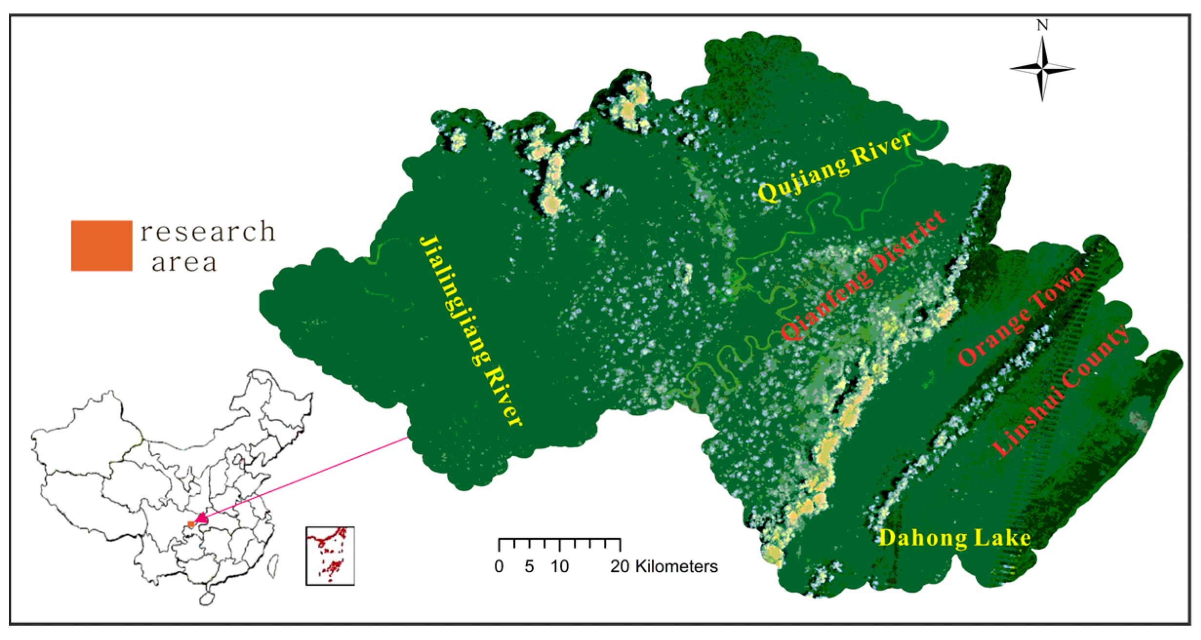
2.1. Overview of the Study Area

Guang’an City is located in a hilly area in the middle of Sichuan Province with a parallel ridge valley area in the east. Within the geographic range of 105°56′–107°19′ E and 30°01′–30°52′ N, it is an area dominated by hilly landforms, with an elevation of 400–1500 m. It is in a subtropical monsoon region with a warm climate and abundant precipitation. There are many lakes and rivers with abundant products. The plants are mostly subtropical evergreen broadleaved forests. The Qujiang River in the middle of Guang’an City and the Jialing River in the southwest are tributaries of the Yangtze River. The NE–SE-oriented Huaying Mountain, Tongluo Mountain, and Mingyue Mountain are arranged in parallel to the east of Guang’an. Guang’an covers an area of 6393.22 km2, consisting of one city, three counties, and two districts. The total population in 2017 was 4.647 million, and the gross national product (GDP) in 2018 was 125.02 billion CNY. Guang’an City is a national garden city, enjoying a good overall ecological environment. The overall ecological structure of Guang’an forests and lakes is mainly distributed across the city, constituting a planar area with high land ecological quality. There are areas with high linear land ecological quality, such as Qujiang River in the middle and Jialing River in the southwest, in addition to the adjacent areas. Basic farmland and economic forest areas are of good land ecological quality. Cities and towns with relatively more construction land and their surrounding areas are of low and medium land ecological quality. A geographic map of Guang’an is shown in Figure 1.

2.2. Data Preprocessing

The remote sensing images, terrain, temperature, precipitation, night lights, GDP, population, NDVI (vegetation index), GPP (vegetation primary productivity), and other relevant data were downloaded from websites such as http://www.gscloud.cn/, http://www.class.ngdc.noaa.gov/, Resource and Environment Data Cloud Platform, and Global Change Scientific Research Data Publishing System (accessed on 5 August 2019).
The remote sensing images were obtained from the Geospatial Data Cloud website, among which eight remote sensing images from Landsat5 in 2000, 2005, and 2010 and Landsat8 in 2015 were downloaded. The Landsat5 TM data level becomes Level 1T after radiation correction and geometric correction with ground control points. Landsat 8 OLI_TIRS data are also a Level 1T product, having undergone terrain correction, radiation correction, and geometric correction. Flash atmospheric correction, mosaic, cutting, and other preprocessing steps were applied to Landsat5 TM and Landsat8 ETM+ data in the paper.
The fractal texture, color, vegetation index, water body index, bare land index, building index, and other features of the remote sensing image were extracted in this study, and the land-use classification was combined with the support vector machine model. The land-use classification map of Guang’an City is shown in Figure 2. The proportion of land-use types in 2000, 2005, 2010, and 2015 is shown in Table 1.
The kilometer grid was used as the evaluation unit in this paper. The steps of importing the evaluation indicators into the kilometer grid were as follows: ① use the FISHNET tool module of ArcGIS 10.3 software to create a kilometer grid with a size of 1 km × 1 km in Guang’an; ② classify the land data assigned to the attribute data of each kilometer grid; ③ assign the terrain, population, GDP, night lights, temperature, NDVI, precipitation, GPP, land-use classification, and other data to the attribute data of each kilometer grid.

3. Methods

3.1. Selection of Evaluation Indicators

This paper comprehensively considered the actual situation of Guang’an City, took the main ecological problems facing Guangan City as a guide, screened various evaluation indicators based on land ecology and other related theories, and established the ecological background, ecological structure, ecological stress, and ecology. The remote sensing evaluation index system was composed of a total of 14 evaluation indices in four criterion layers, as shown in Table 2.

3.2. Subjective and Objective Weighting

There are many calculation methods for evaluating index weight values, which are mainly divided into two categories, subjective methods and objective methods. ① The Delphi method [14] is a comprehensive weighting method that combines the experience and subjective opinions of experts. ② The entropy weight method uses objective weighting. The concept of ’entropy’ was first proposed by the German physicist Clausius [15] in 1865, which mainly reflects the uniformity of the physical energy distribution in space. A more uniform energy distribution results in higher entropy values. The concept of information entropy was proposed later. It was first introduced to information theory by Shannon in 1945, and it was mainly used to describe the uncertainty of the source signal at first [16].
This paper used subjective and objective methods to calculate the weight of each evaluation index. This method could avoid the one-sidedness caused by using subjective or objective weighting methods alone, and it combined the advantages of the two methods. The calculation formula of the subjective and objective combination method is as follows:
W i = α U i + β V i
where U is the weight value calculated using the Delphi method, V is the weight value calculated using the entropy weight method, i is the serial number of the evaluation index, and α , β are the combined coefficients of the subjective method and the objective method, respectively. The constraint condition of α and β is α 2 + β 2 = 1 .

3.3. Classification of Land Ecological Quality Using Ideal Point Method

The ideal point method is an evaluation function method for solving multi-objective programming problems in which each objective value is approximated as close as possible to its ideal (optimal) value [17].
At present, the comprehensive index method model is a mathematical evaluation model that is widely used in the evaluation of land ecological quality [4], and it has the advantages of simplified calculation, small information loss, and easy comparison and analysis of the evaluation indicators in the vertical and horizontal directions. The ideal point method is one of the comprehensive index evaluation methods, and it is also a highly practical multi-index mathematical modeling method. The specific algorithm is outlined below.
(1) Establish a decision matrix (such as km grid attribute table). Assuming that the number of evaluation units is i and the number of evaluation indices is j, after standardizing the evaluation index data, a multi-attribute (multi-index standardized value) decision matrix A can be established.
A = | r 11 r 12 r 1 n r 21 r 22 r 2 n r m 1 r m 2 r m n |
where rmn is the normalized value of the n evaluation index in the m evaluation unit in the formula.
(2) Establish an ideal value point and an evaluation point in the N-dimensional Euclidean space so that the value of each component of the ideal point vector is 1. In the evaluation point vector, the calculation formula of the positive index is X = X X min X max X min , and the formula for calculating the negative indicator is X = 1 X X min X max X min . In step (1), the evaluation index data are standardized, and the normalized values of positive and negative indicators are distributed in the [0–1] interval. After the calculation of negative indicators, the negative indicators become positive indicators, and the ideal values of positive with negative indicators can be assigned to 1, thereby reducing the calculation complexity of the model.
(3) According to the above subjective and objective weighting method, calculate the weighted value of each evaluation index in each evaluation unit to obtain the evaluation vector. Finally, calculate the Euclidean distance between the evaluation vector and the ideal point vector, whose calculation formula is
D = j = 1 m ( 1 V i j ) 2   ( i = 1 , 2 , , n )
where D is the Euclidean distance value, and Vij is the weighted value of the j evaluation index in the i evaluation unit.
(4) According to the Euclidean distance of each evaluation unit calculated in step (3), the natural breakpoint method is used to divide the ecological grade of each evaluation unit.
The ideal point method has no limitation on the number of evaluation units and evaluation indices in the application of multi-index comprehensive evaluation, and it is convenient to compare the evaluation content vertically and horizontally; thus, it has a wide range of application. The calculation efficiency of the ideal point model is improved using the traditional ideal evaluation model in steps (2) and (3), and the impact of the four criteria layers of ecological background, ecological structure, ecological benefits, and ecological stress on land ecological quality can be better described, making the ecological assessment more accurate.

3.4. Hot Spot Analysis Model

The hot spot analysis model was first proposed by the spatial metrologist Anselin in 1995. It is a spatial correlation local index based on the spatial autocorrelation theory of spatial metrology geography. At present, the hot spot analysis model has been widely used in the study of the spatial differentiation of natural factors. Its steps are as follows: ① calculate the local high and low cluster values of natural factors; ② calculate the high and low cluster values of the natural factor aggregation degree or aggregation difference. The calculation formula for hot and cold spots is as follows:
G i * d = j = 1 n ω i j ( d ) x j / j = 1 n x j
It is necessary to standardize G i * in order to make the local maximum and minimum values reflected by the cold and hotspot values obtained in the above formula more accurate, and the formula is as follows:
Z ( G i * ) = G i * E ( G i * ) V a r ( G i * )
where Var(Gi*) is the variance value of Gi*, E(Gi*) is the mathematical expectation value of Gi*, and xj is the ideal point value of each evaluation unit of land ecological quality. If the value of Z(Gi*) is positive and significant, it indicates that the local extremely high clustering value of point i is high, and that point i is a hot spot. However, if the value of Z(G*) is negative and significant, it indicates that the local extremely low clustering of point i is low, and that point i is a cold spot. The spatial differentiation of land ecological quality in general regions generally shows the spatial distribution characteristics of ‘core–edge’.
The hot spot analysis model is mainly used to study the spatial differentiation of natural elements. The basic idea is to calculate the distribution of nearby natural elements. The extremely high-value clustering area is a hot spot aggregation area. When the natural elements meet the cluster value, natural elements with an extremely high cluster value are surrounded by other regions of high cluster value, and this extremely high cluster value is called a hot spot with statistical significance. Similarly, cold spots are opposite to hot spots. If the sum of the hot spot and the surrounding natural elements differs greatly from the expected sum of the adjacent areas of the natural elements, this high aggregate value is a statistical hot spot score.

3.5. Analyses of Main Control Factors

Principal component analysis is a multivariate statistical method to investigate the correlation of multiple variables. It reveals the internal structure of multiple variables through a few principal components, i.e., it derives a few unrelated principal components from the original variable so as to retain as much information as possible of the original variable. The typical mathematical treatment is to take the original P index as a linear combination, generating a new comprehensive index.
The principal component analysis method was used to extract the main controlling factors of land ecological quality in this paper. The principal component analysis method is a statistical method used for data dimensionality reduction. The algorithm proceeds as follows: ① perform spatial transformation (orthogonal transformation); ② convert the original random vector component correlation into a new irrelevant random vector component, so as to transform the covariance matrix into a diagonal matrix from the perspective of algebra. This allows orthogonally transforming the coordinate system from the perspective of solid geometry, where the new random vector in the new coordinate system represents the most scattered sample points (the N orthogonal directions with the largest variance) to achieve data dimensionality reduction, so as to obtain a low-dimensional system with higher accuracy; ③ convert the low-dimensional variable system into a one-dimensional variable system by creating a value function [18].
The principal component analysis method can transform a multivariable system into a new variable system with a small number. These few new variables contain most of the information of the original multivariable system. The land ecological quality evaluation system is also a multivariable (evaluation index) system. The principal component analysis method can transform this multivariable system into a system composed of a few variables through orthogonal transformation, and this system of few variables also includes most of the information of the original land on multiple evaluation indicators of ecological quality. The principal component analysis method can form independent principal components after performing orthogonal transformation, which eliminates the correlation among multiple evaluation indices. In the principal component analysis method, the contribution rate weight of each principal component represents the proportion of the information contained in the principal component in the original total information, and the contribution rate weight is objective and data-driven.

4. Results and Discussion

4.1. Classification of Ideal Points for Land Ecological Quality

This paper used MATLAB2016a software programming to calculate the ideal point value (land ecological quality evaluation value) of each evaluation unit, and then the natural breakpoint method in ArcGIS 10.3 software was used to classify the ideal point value of each kilometer grid. There are 7012 evaluation units within the scope of Guang’an City, and the ideal point value of each evaluation unit was divided into five grades from low to high using the natural break point method: grade 1 (poor), grade 2 (general), grade 3 (medium), grade 4 (good), and grade 5 (excellent), along with five other ecological quality grades. The grade maps of the ideal points of land ecological quality in four phases of 2000, 2005, 2010, and 2015 are shown in Figure 3.
The MATLAB2016a software programming was used in the paper to obtain the proportion of the number of evaluation units in each grade of four phases in 2000, 2005, 2010, and 2015. The proportion of evaluation units of each ecological level in 2000, 2005, 2010, and 2015 are shown in Table 3.

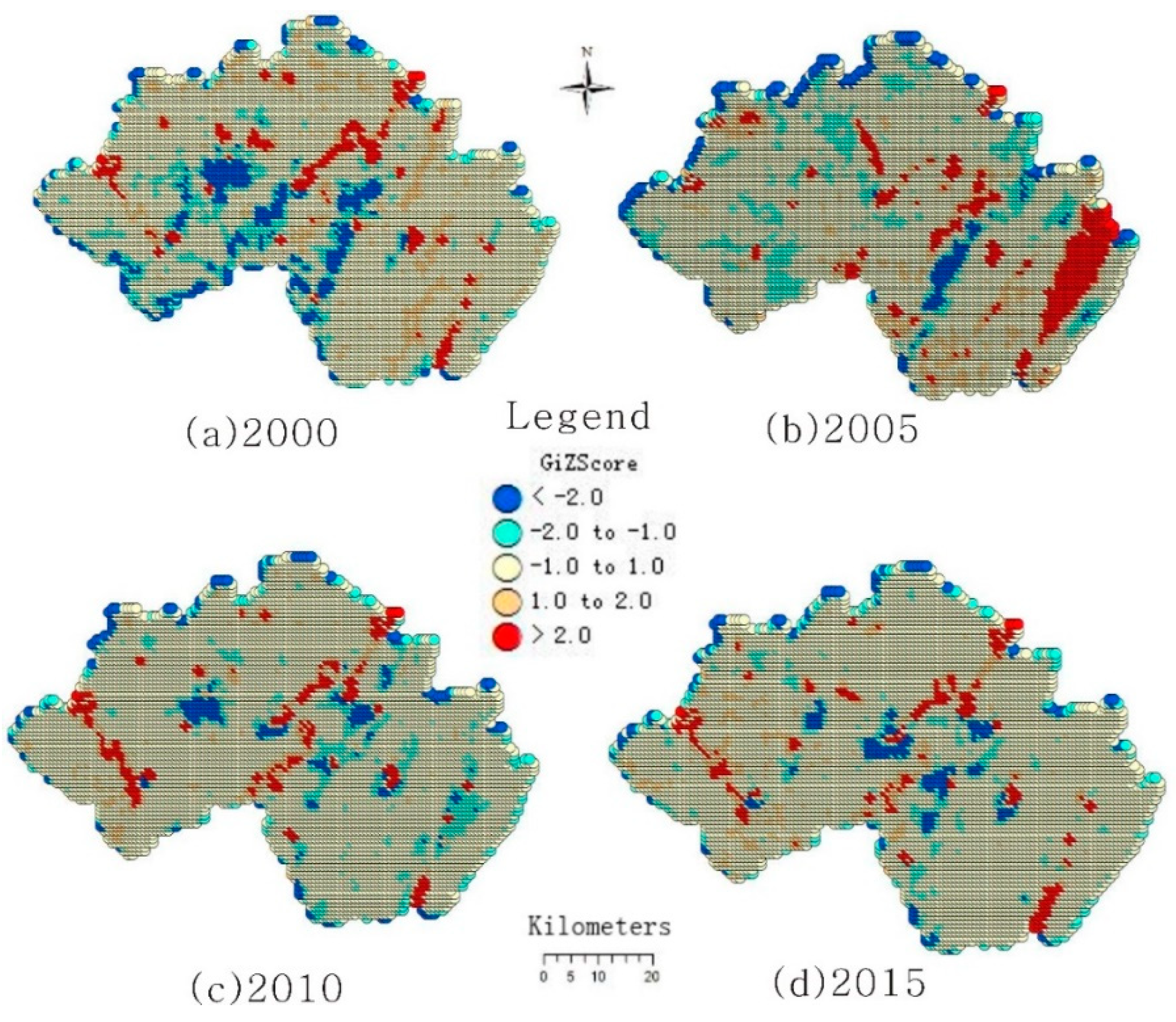
4.2. Spatial Differentiation Analysis of Land Ecological Quality Based on Hot Spot Model

The steps to obtain the hot spot values were as follows: (1) take the land ecological quality evaluation value (ideal point value) as the basic data; (2) use ArcGIS 10.3 software and the hot spot analysis tool in the toolbox (Arctoolbox) to calculate the hot and cold spot values of the ideal point values of land ecological quality in 2000, 2005, 2010, and 2015; (3) render the cold and hot spot values into a map by layers, and obtain the spatial differentiation maps of hot spots in Guang’an in 2000, 2005, 2010, and 2015 (as shown in Figure 4).
It can be seen from Figure 4 that the land ecological quality in Guangan City in 2000, 2005, 2010, and 2015 differed extensively. The high-value clustering area is a hot spot area indicating better land ecological quality. The low-value clustering area is a cold spot area indicating poorer ecological quality. The area with the highest hot spot value can be set as the fifth-level distribution area of land ecological quality. The fifth-level area had the best land ecological quality in Guang’an City. On the contrary, the local area with the lowest hot spot value (first-grade distribution area) was the area with the worst land ecological quality. The land ecological quality was positively correlated with the corresponding hot spot value.

4.3. Analyses of Main Control Factors

In this paper, the main component analysis function of SPSS22 software was used to extract the four main controlling factors of land ecological quality in Guangan City in 2000, 2005, 2010, and 2015. The steps are shown as follows: (1) SPSS22 software was used to import the decision matrix corresponding to each evaluation unit in each phase of Guang’an City, which was established using the standardized value of multi-evaluation index, and the threshold value was set to 1, indicating that the variance of the principal component analysis method was greater than 1. The vector was set as the main component; (2) the evaluation index (factor) corresponding to the position with the highest score in the first few main component vectors was set as the main control factor. The main control factors in 2000, 2005, 2010, and 2015 are shown in Table 4, Table 5, Table 6 and Table 7, respectively, in which the component order was sorted according to the magnitude of the value in the first main component vector. In these tables, (+) in the main control factor represents a positive factor, while (−) indicates a negative factor. FAC1_1, FAC2_1, and FAC3_1 indicate the first, second, and third principal components, respectively.
According to Table 4, Table 5, Table 6 and Table 7, the evaluation index corresponding to the maximum value in each column of the first three principal components FAC_1-1, FAC_2-1, and FAC_3-1 was taken as the main control factor. The main control factors in 2000, 2005, 2010, and 2015 are shown in Table 8.

4.4. Comprehensive Evaluation

Through this study, we obtained the grades of land ecological quality ideal points in 2000, 2005, 2010, and 2015 and the ecological main control factors of each year, on the basis of which the relationship between the proportion of ideal points in each stage and the corresponding main control factors was determined. The results of the comprehensive analysis and evaluation are outlined below.
(1) As can be seen from Figure 3 and Table 3, the ecological quality in most of the areas of Guang’an in various years was concentrated in grades 2 and 3, with a total proportion of approximately 90%. The proportion of areas in grade 5 in each year was relatively low, constituting less than 1%. The proportions of grades 2 and 3 were roughly negatively correlated. The proportions of grade 2 area increased to a certain extent in 2000 to 2005. The proportions of grade 4 increased slightly in 2000 to 2005, decreased slightly in 2005 to 2010, and increased slightly in 2010 to 2015. Grade 1 was roughly negatively correlated with the proportion of grade 4 area. In general, the proportion of grade 3 area was the largest overall and typically increased; thus, the land ecological quality in Guang’an City improved from 2000 to 2015.
(2) The relationship between the proportion of each grade area of the ideal point and the main control factors was evaluated. It can be seen from the main control factors of each year in Table 8 that, except for the first main control factor temperature in 2005, forest land was the most important main controlling factor for land ecological quality in the region. The temperature in 2005 increased compared with 2000 according to the data preprocessing results in this paper. It can be seen from Table 3 that the area proportion of grade 3 ecological quality increased with temperature in 2005, indicating a positive correlation. Since grade 3 was largest in terms of area proportion, its increase also represented an improvement of the overall land ecological quality, indicating that the overall temperature is positively correlated with land ecological quality. In short, the proportion and temperature of forest land were the main controlling factors for land ecological quality in Guang’an City. The proportion of forest land and temperature were positively correlated with land ecological quality.
(3) According to Figure 1 and Figure 4, as well as Table 8, the overall land ecological quality differentiation law of Guang’an City showed that hot spots were mainly distributed along three lines, all of which were water bodies such as Qujiang River, Jialing River, and Dahong Lake. The distribution area of hot spots in the eastern mountainous area increased accordingly, and the hot spots indicated the highest ecological quality. Cold spots were generally distributed in Guang’an and the surrounding counties and towns, which were the areas with the lowest land ecological quality.
The distribution areas of hot spots along the Qujiang River, Jialingjiang River, and Dahong Lake areas decreased significantly from 2000 to 2005. Hot spots distributed in the area near Orange Town in Linshui County increased, while cold spots around the urban area of Guang’an City increased. This decrease may be related the temperature increase in 2005. From 2005 to 2010, the hot spots increased significantly along the Qujiang River, Jialing River, and Dahong Lake areas, while the cold spots increased around the urban areas of Guang’an and the Qianfeng District, which may be related to the temperature drop in 2010. From 2010 to 2015, the distribution area of hot spots near Qujiang River, Jialingjiang River, and Dahong Lake decreased significantly, while that of cold spots decreased significantly in the urban area of Guang’an City and its surrounding counties and towns.
(4) The spatial differentiation of hot spots was found to be constrained by certain master control factors. According to Table 8 and Figure 4, the temperature increased significantly from 2000 to 2005, and the overall area of hot spot distribution also increased significantly. Specifically, it increased in the surrounding areas of Orange Town in Linshui County, whereas it decreased significantly in the areas along the Qujiang River and Jialing Rivers. The distribution area of cold spots decreased significantly in the urban areas of Guang’an City and its surrounding counties and towns. From the analysis above, it can be concluded that ① the proportion of forest land area and temperature were positively correlated with land ecological quality, and they were the most important main control factors, ② temperature was negatively related to the overall land ecological quality in the riverside areas of the western and central water bodies of Guang’an City, and ③ ecological hot spots were generally distributed in the areas along the Qujiang River and Jialing Rivers and the mountainous areas in the east.

5. Conclusions

The comprehensive analysis and evaluation of the land ecological quality in 2000, 2005, 2010, and 2015 showed that ① the overall quality of land ecology increased, ② the proportion of forest land and temperature were the most important main control factors for land ecological quality, all of which were positively correlated, ③ temperature was negatively correlated with the overall land ecological quality in the riverside areas of the western and central water bodies of Guang’an City, and ④ ecological hot spots were generally distributed in the areas along the Qujiang River and Jialingjiang River and the mountainous areas in the east.
The main research contributions are as follows: (1) the subjective and objective combination method was used to calculate the weight of each land ecological evaluation index, which avoided the one-sidedness caused by using subjective or objective weighting alone, and this improved the accuracy of evaluation index weight calculation. Furthermore, it had certain innovative features. (2) This paper improved the traditional ideal point model, set the ideal value of all evaluation indicators to 1, and then calculated the Euclidean space distance from the evaluation index vector to the ideal point vector, which reduced the calculation amount of the land ecological quality evaluation model.

Author Contributions

Conceptualization, Z.C.; Methodology, Z.C.; Formal analysis, Z.C.; Data curation, L.S. All authors have read and agreed to the published version of the manuscript.

Funding

This research received no external funding.

Institutional Review Board Statement

I choose to exclude this statement.

Informed Consent Statement

I choose to exclude this statement.

Data Availability Statement

I choose to exclude this statement. The source of the data has been introduced in Section 2.2.

Conflicts of Interest

The authors declare no conflict of interest.

References

  1. Pieri, C.; Dumanski, J.; Hamblin, A.; Young, A.; Undp, U. Land Quality Indicators. World Bank Discuss. Pap. 1995, 81, 81. [Google Scholar]
  2. Messing, I.; Fagerström, M.-H.H.; Chen, L.; Fu, B. Criteria for land suitability evaluation in a small catchment on the Loess Plateau in China. Catena 2003, 51, 215–234. [Google Scholar] [CrossRef]
  3. Zhang, J.Y.; Su, W.C.; Zhang, F.T. Evaluation of Land Ecological Security in the Three Gorges Reservoir Ecological Economic Zone based on PSR Model. China Environ. Sci. 2011, 31, 1039–1044. [Google Scholar]
  4. Paracchini, M.L.; Pacini, C.; Jones, M.L.M.; Pérez-Soba, M. Aggregation framework to link indicators associated with multifunctional land use to the stakehode: Evaluation of options. Ecol. Indic. 2011, 1, 71–80. [Google Scholar] [CrossRef]
  5. Gong, F.; Chen, B. Research on comprehensive evaluation of grassland ecological compensation based on DPSIR model——Taking Inner Mongolia as an example. J. Inn. Mong. Agric. Univ. (Soc. Sci. Ed.) 2019, 21, 1–6. [Google Scholar]
  6. Zou, Y.; Zhu, D.; Chen, W.; Sun, Z. Evaluation of environmental efficiency and ecological inefficiency of various regions in China based on DEA model. J. Hubei Univ. (Nat. Sci. Ed.) 2020, 42, 12–19+26. [Google Scholar]
  7. Wang, Y.; Wei, J.; Sun, Q.; Wang, F. Evaluation and prediction of ecological security based on ARIMA-ANN model—Taking Hexi Corridor urban agglomeration as an example. J. Ecol. 2020, 39, 326–336. [Google Scholar]
  8. Feng, W.B.; Li, S.F. Research on evaluation of land ecological security in Jiangsu Province. Bull. Soil Water Conserv. 2013, 33, 285–290. [Google Scholar]
  9. Li, L.; Hou, S.T.; Zhao, Y.; Zheng, X. Evaluation and prediction of land ecological security in Henan Province based on P-S-R Model. Res. Soil Water Conserv. 2014, 21, 188–192. [Google Scholar]
  10. Li, Y.Y.; Yang, C.X.; Xin, G.X.; Liu, S.; Zhao, T. Research on the dynamic changes of land ecological security. J. Southwest China Norm. Univ. (Nat. Sci. Ed.) 2014, 39, 189–195. [Google Scholar]
  11. Lu, L.F.; Yan, L.J. Evaluation of land ecological security in county areas: Taking Danling County, Sichuan Province as an Example. J. Ecol. Rural. Environ. 2013, 29, 295–300. [Google Scholar]
  12. Dai, L.; Yao, X.C.; Zhou, S.L.; Li, L. Evaluation of the ecological status of land in Jintan City, an economically developed area of the Yangtze River Delta. Trans. Chin. Soc. Agric. Eng. 2013, 29, 249–257. [Google Scholar]
  13. Chen, Z.; Xia, X.Q.; Chen, J.P. Remote Sensing Evaluation Model and Main controlling factors of land Ecological quality: A case study of Guang’ an City. Remote Sens. Land Resour. 2021, 33, 201–208. [Google Scholar]
  14. Yu, Y.; Zhou, D.M.; Wang, H.; Sun, N. Analysis of land resource evaluation method and determination of evaluation factor weight. Chin. J. Eco-Agric. 2006, 213–215. [Google Scholar]
  15. Guo, Q.; Wang, Q.; Lan, H. Preliminary research on ecosystem entropy. Liaoning Meteorol. 1992, 21, 9–10. [Google Scholar]
  16. Wang, Q.Y.; Pan, X.H. Application of entropy weight method in emergency rescue assessment of major hazard sources. J. Nanjing Univ. Technol. (Nat. Sci. Ed.) 2011, 33, 87–92. [Google Scholar]
  17. Wang, S.H.; Zhu, B.Q.; Zhang, Z. Rock mass disjointed plane classification method based on improved ideal point model. J. Northeast. Univ. Nat. Sci. Ed. 2021, 42, 117. [Google Scholar]
  18. Chen, Z.; Li, S.; Chen, J. Remote Sensing Spatial Differentiation and Main controlling Factors of land Ecological quality: A case study of Guang’ an City. Bull. Surv. Mapp. 2020, 6, 94. [Google Scholar]
  19. Huang, H.; Luo, W.; Wu, C.; Li, D. Evaluation of land ecological security based on matter element analysis. Trans. Chin. Soc. Agric. Eng. 2010, 26, 316–322. [Google Scholar]
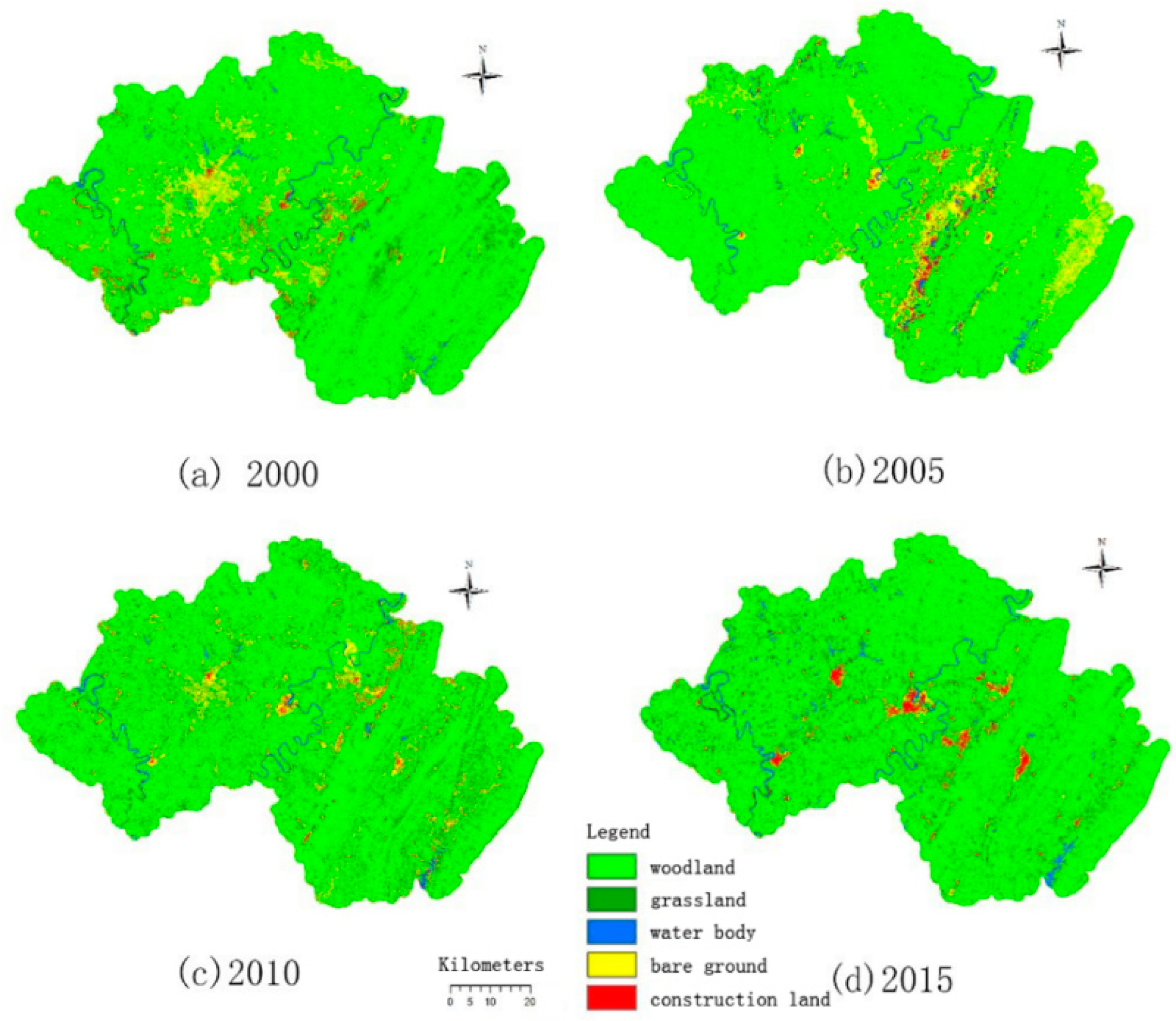
Figure 1. Administrative map of Guang’an city.
Atmosphere 13 01955 g001
Figure 2. The land classification map of the study area in the four years of 2000, 2005, 2010, and 2015 [13]. (a) The land classification map of the study area in 2000 (b) The land classification map of the study area in 2005 (c) The land classification map of the study area in 2010 (d) The land classification map of the study area in 2015.
Atmosphere 13 01955 g002
Figure 3. Grade map of ideal points in 2000, 2005, 2010, and 2015 [19].(a) Grade map of ideal points in 2000 (b) Grade map of ideal points in 2005 (c) Grade map of ideal points in 2010 (d) Grade map of ideal points in 2015.
Atmosphere 13 01955 g003
Figure 4. The spatial differentiation maps of cold and hot spots in 2000, 2005, 2010, and 2015 [19].(a) The spatial differentiation maps of cold and hot spots in 2000 (b) The spatial differentiation maps of cold and hot spots in 2005 (c) The spatial differentiation maps of cold and hot spots in 2010 (d) The spatial differentiation maps of cold and hot spots in 2015.
Atmosphere 13 01955 g004
Table 1. The proportion of land-use types in 2000, 2005, 2010, and 2015.
YearsProportion of Land-Use Types (%)
WoodlandGrasslandWaterWastelandConstruction Land
200079.076.682.559.751.95
200582.990.263.5611.431.76
201079.338.652.756.422.85
201585.794.444.391.843.54
Table 2. Remote sensing evaluation index system for land ecological quality.
Criterion LayerEvaluation Index
Ecological background1. Average annual precipitation; 2. annual average temperature; 3. vegetation index; 4. total primary productivity (GPP); 5. topography
Ecological structure6. Proportion of forest land; 7. proportion of grassland; 8. proportion of water body; 9. proportion of bare land; 10. proportion of construction land
Ecological benefits11. The value of ecological services
Ecological stress12. Gross domestic product (GDP); 13. population density; 14. night lights
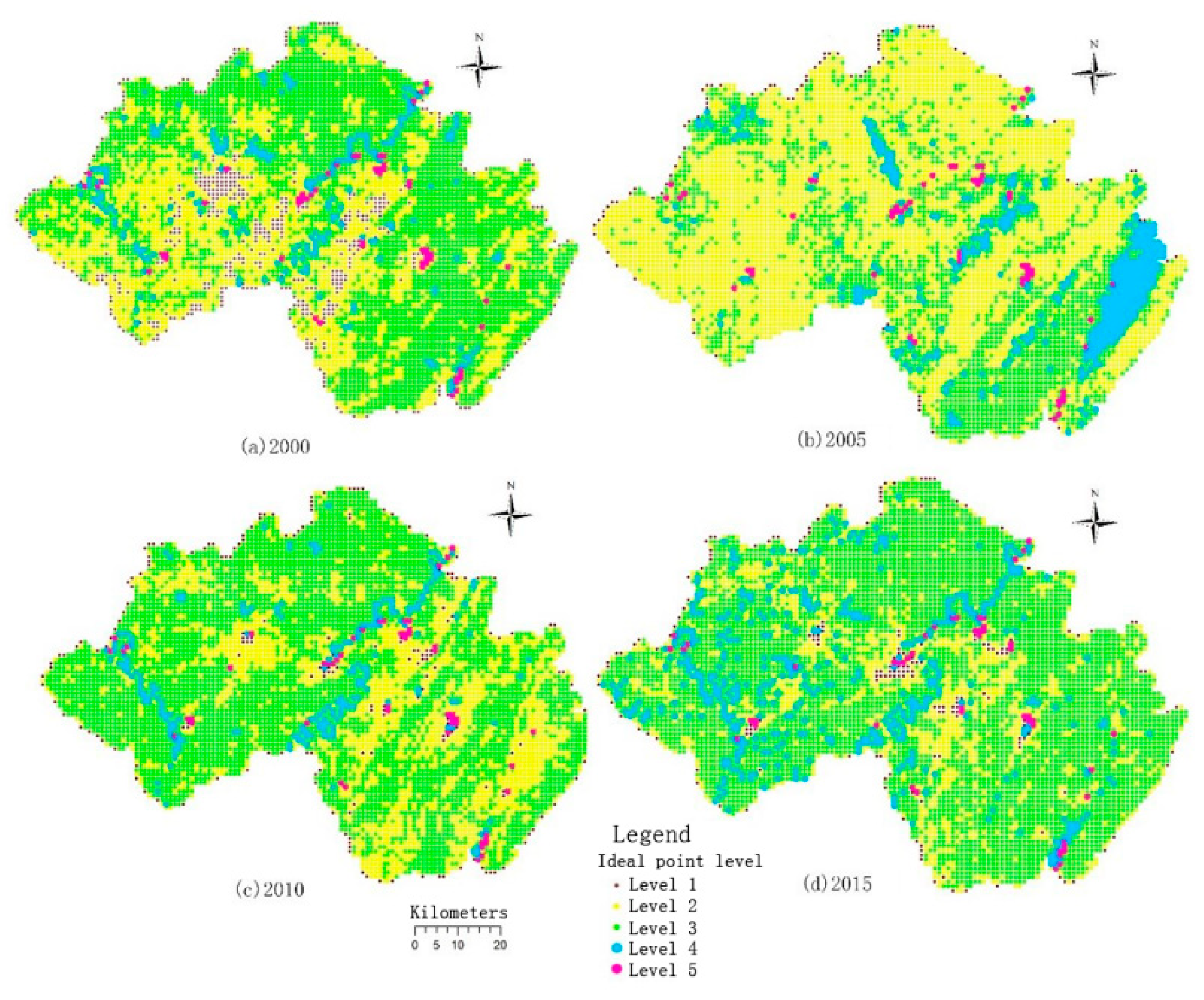
Table 3. The table for the proportion of evaluation units of each ecological level in 2000, 2005, 2010, and 2015.
Ecological GradeProportion of Evaluation Units (%)
2000200520102015
Level 17.071.252.762.61
Level 233.7956.5228.6017.04
Level 354.8434.7464.5972.41
Level 43.426.613.227.13
Level 50.810.830.760.71
Table 4. Main control factors in 2000.
Master FactorOrder of ComponentsFAC1_1FAC2_1FAC3_1
Terrain (−)−0.308 07−0.026 89−0.342 47
Population (−) −0.520 77−0.338 18−0.716 06
GDP (−) −0.424 16−0.243 47−0.569 85
Night lights (−) −0.329 16−0.154 92−0.482 63
Air temperature (+) 0.595 200.562 660.544 18
NDVI (+) 0.433 000.306 73−0.123 04
Precipitation (+) 0.482 340.426 820.288 68
GPP (+) −0.844 80−0.569 17−1.084 96
Proportion of woodland (+)12.955 60−0.599 57−0.172 50
Proportion of grassland (+) −0.600 230.175 69−0.762 56
Proportion of water (+)3−0.695 58−1.952 642.563 03
Proportion of wasteland (+)2−0.399 692.579 521.348 87
Proportion of construction land (−)−0.343 67−0.166 58−0.490 69
Table 5. Main control factors in 2005.
Master FactorOrder of ComponentsFAC1_1FAC2_1FAC3_1
Terrain (−)30.336 04−0.333 251.884 00
Population (−) −0.336 63−0.240 460.412 78
GDP (−) 0.215 26−0.319 191.442 95
Night lights (−) −0.071 25−0.289 970.836 87
Air temperature (+)12.581 45−0.147 24−0.860 66
NDVI (+) −0.394 08−0.349 280.012 99
Precipitation (+) 1.390 53−0.139 22−0.949 99
GPP (+) −0.883 23−0.240 13−1.551 93
Proportion of woodland (+) −0.211 710.464 050.333 61
Proportion of grassland (+) −0.862 01−0.087 26−0.959 10
Proportion of water (+) −0.892 80−0.247 32−0.530 70
Proportion of wasteland (+)2−0.100 583.297 760.220 05
Proportion of construction land (−)−0.770 99−0.263 21−0.290 85
Table 6. Main control factors in 2010.
Master FactorOrder of ComponentsFAC1_1FAC2_1FAC3_1
Terrain (−) −0.315 20−0.063 57−0.386 22
Population (−) −0.521 95−0.052 42−0.896 30
GDP (−) −0.433 11−0.07 549−0.723 02
Night lights (−) −0.295 67−0.061 55−0.671 06
Air temperature (+) 0.585 50−0.244 600.996 77
NDVI (+) 0.602 72−0.446 480.634 94
Precipitation (+) 0.491 46−0.276 410.736 05
GPP (+) −0.849 940.093 58−1.650 53
Proportion of woodland (+)12.906 750.445 09−0.69 235
Proportion of grassland (+) −0.503 90−1.160 840.437 99
Proportion of water (+)2−0.682 322.986 161.131 55
Proportion of wasteland (+)3−0.614 83−1.083 001.739 95
Proportion of construction land (−)−0.369 50−0.060 47−0.657 77
Table 7. Main control factors in 2015.
Master FactorOrder of ComponentsFAC1_1FAC2_1FAC3_1
Terrain (−) −0.302 46−0.247 350.037 47
Population (−) −0.443 68−0.416 520.302 54
GDP (−) −0.378 95−0.363 770.244 99
Night lights (−) −0.268 11−0.317 800.584 07
Air temperature (+) 0.532 440.156 52−1.461 93
NDVI (+) 0.513 35−0.067 13−0.423 64
Precipitation (+) 0.493 810.029 23−1.366 81
GPP (+)3−0.804 23−0.539 671.890 78
Proportion of woodland (+)12.937 22−0.105 740.921 57
Proportion of grassland (+) −0.719 98−0.533 020.016 33
Proportion of water (+)2−0.477 373.247 150.346 06
Proportion of wasteland (+) −0.764 16−0.513 73−1.589 99
Proportion of construction land (−)−0.317 88−0.328 190.498 56
Table 8. Main control factors in 2000, 2005, 2010, and 2015.
YearsMaster Factor 1Master Factor 2Master Factor 3
2000Proportion of woodlandProportion of wastelandProportion of water
2005Air temperatureProportion of wastelandterrain
2010Proportion of woodlandProportion of waterProportion of wasteland
2015Proportion of woodlandProportion of waterGPP
Publisher’s Note: MDPI stays neutral with regard to jurisdictional claims in published maps and institutional affiliations.

