Application of Large Time Step TVD High Order Scheme to Shallow Water Equations

Abstract

The numerical modeling of actual river floods faces three challenges related to computational efficiency, accuracy, and proper balancing of terms in the governing equations, all of which are discussed in this paper. Herein, a large time step (LTS) scheme is used to improve efficiency, a high order scheme is used to enhance accuracy, and specific treatment of the bed slope term achieves a well-balanced form of shallow water equations. The LTS scheme, originally proposed by LeVeque in 1998, has led to the development of highly efficient computational solvers of the shallow water equations (SWEs). This paper examines use of a total variation diminishing (TVD) high order scheme in conjunction with LTS. We first applied the scheme to the solution of the homogeneous 1D SWEs and obtained satisfactory results for three cases, even though small oscillations nevertheless occur when the CFL number is very large. The additional source term makes the issue more complicated and can introduce a spurious flow when the term is not correctly handled. Many methods have been developed in traditional differential schemes, but not all are fit for the TVD-LTS scheme; for example, the method of decomposing the source term into simple characteristic waves has proved infeasible. In this paper the TVD-LTS scheme was implemented for the first time for well-balanced SWEs containing bed slope source terms. We found that oscillations were not as suppressed as for the homogeneous SWEs when the TVD-LTS scheme was applied to the three cases of step Riemann problems (SRP) tested for CFL numbers 1 to 10. For free surface flow over a bed hump, the TVD-LTS scheme can only reach CFL number 4 before the solution breaks down.

1. Introduction

Shallow water equations (SWEs) are depth-integrated continuity and momentum equations for river flow, in which it is assumed that surface waves are long, the depth is relatively small in comparison with the horizontal scale of the flow domain, and the pressure is hydrostatic. In the version considered in the present paper, viscous terms are neglected, which restricts the applicability of the equations but is acceptable for a wide range of flows in open channel hydraulics (see, e.g., Abbott and Minns [1] and Toro [2]). The SWEs can be formulated as a nonlinear hyperbolic system that can be discretized using an upwind method such as the Roe [3], Osher [4], and AUSM [5] schemes. Alternative higher-order schemes such as WENO [6,7] also work by reconstruction, using additional cells next to the interface. However, all the foregoing schemes are constrained by a time step stability condition, such as the Courant–Frederichs–Lewy number CFL < 1, where CFL = u_maxΔt/Δx, in which u_max is the maximum flow speed, Δt is the time step, and Δx is a spatial increment in the computational mesh. In the 1980s, LeVeque [8,9] proposed the large time step (LTS) method, which led to considerable gains in computational efficiency. In practice, LTS does not conflict with CFL theory in that the interface flux is computed across multiple cells in LTS rather than a single cell in traditional schemes, thus enabling the time step to be increased accordingly. In LTS, more cells take part directly in the computation of fluxes, unlike higher-order schemes that use reconstruction schemes to handle cells adjacent to the interface. Murillo et al. [10] and Morales-Hernández [11,12,13] then applied LTS to solve the SWEs for free surface flows, and similarly, Qian [14] used LTS in solving the Euler equations in aerodynamics. All the foregoing LTS schemes are first order. However, as the CFL number becomes large, spurious oscillations appear in the solution, which do not occur in traditional first-order schemes. Harten introduced the total variation diminishing (TVD) concept [15] that could suppress oscillations for second- or higher-order schemes in the traditional form. Harten [16] then proposed a TVD-LTS scheme that was further developed by Qian and Lee [17].

Godunov-type solvers of the SWEs can generate non-physical flow phenomena from discretized bed slope source terms that are out of balance with the flux gradient terms. Well-balanced schemes overcome such difficulties. LeVeque [18] proposed a quasi-steady wave propagation method that incorporated source terms within high-resolution Godunov methods and obtained accurate results for the propagation of small perturbations. Hubbard and García-Navarro [19] utilized a flux difference splitting method to ensure the flux gradient and source terms were correctly balanced. Zhou et al. [20] suggested a surface gradient method to represent the bed slope source term. Rogers et al. [21] presented an algebraic technique for balancing the flux gradient and source terms for single waterbodies. Liang et al. [22] extended the algebraic technique to multiple waterbodies, with stage and discharge selected as dependent variables.

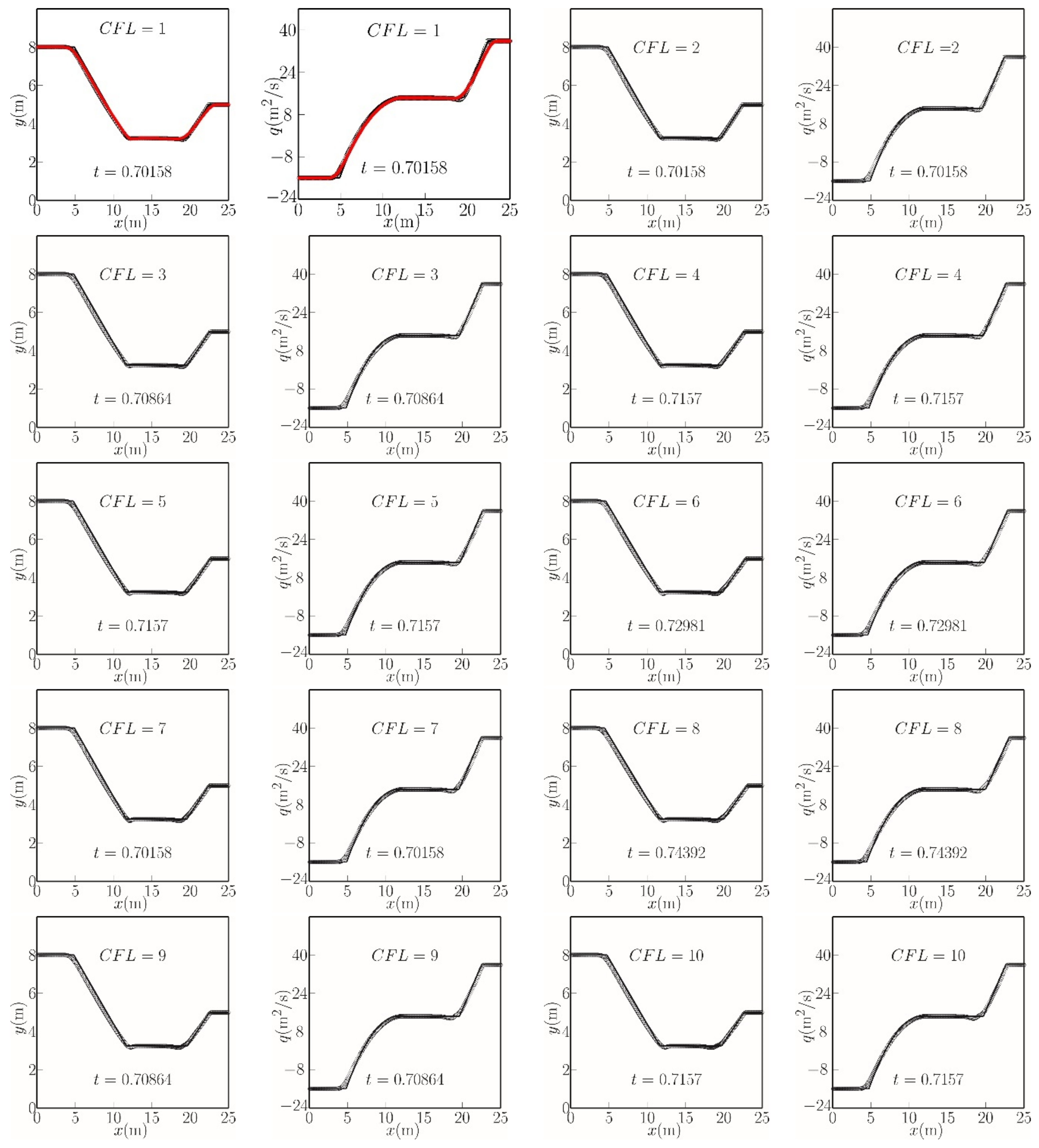
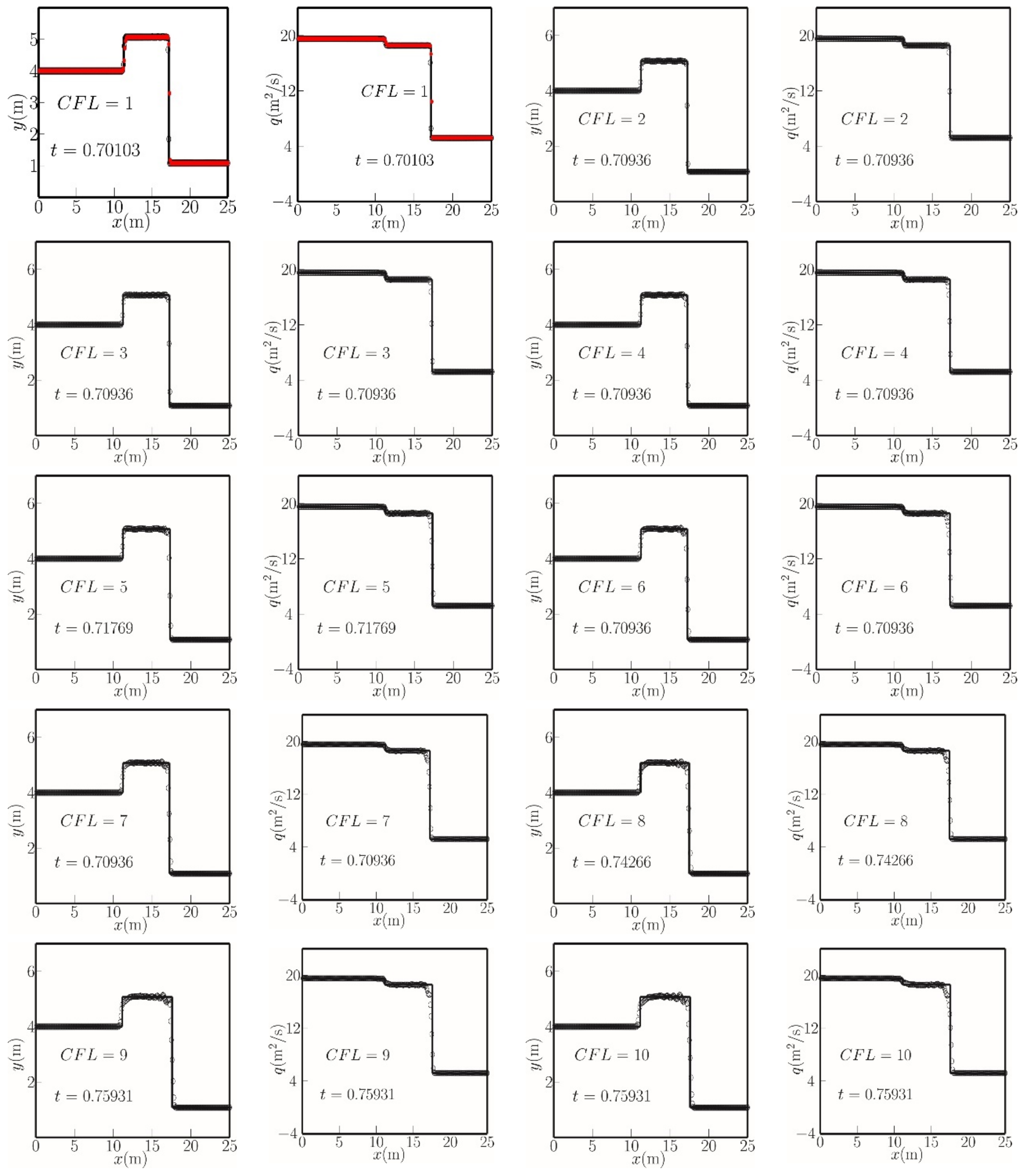
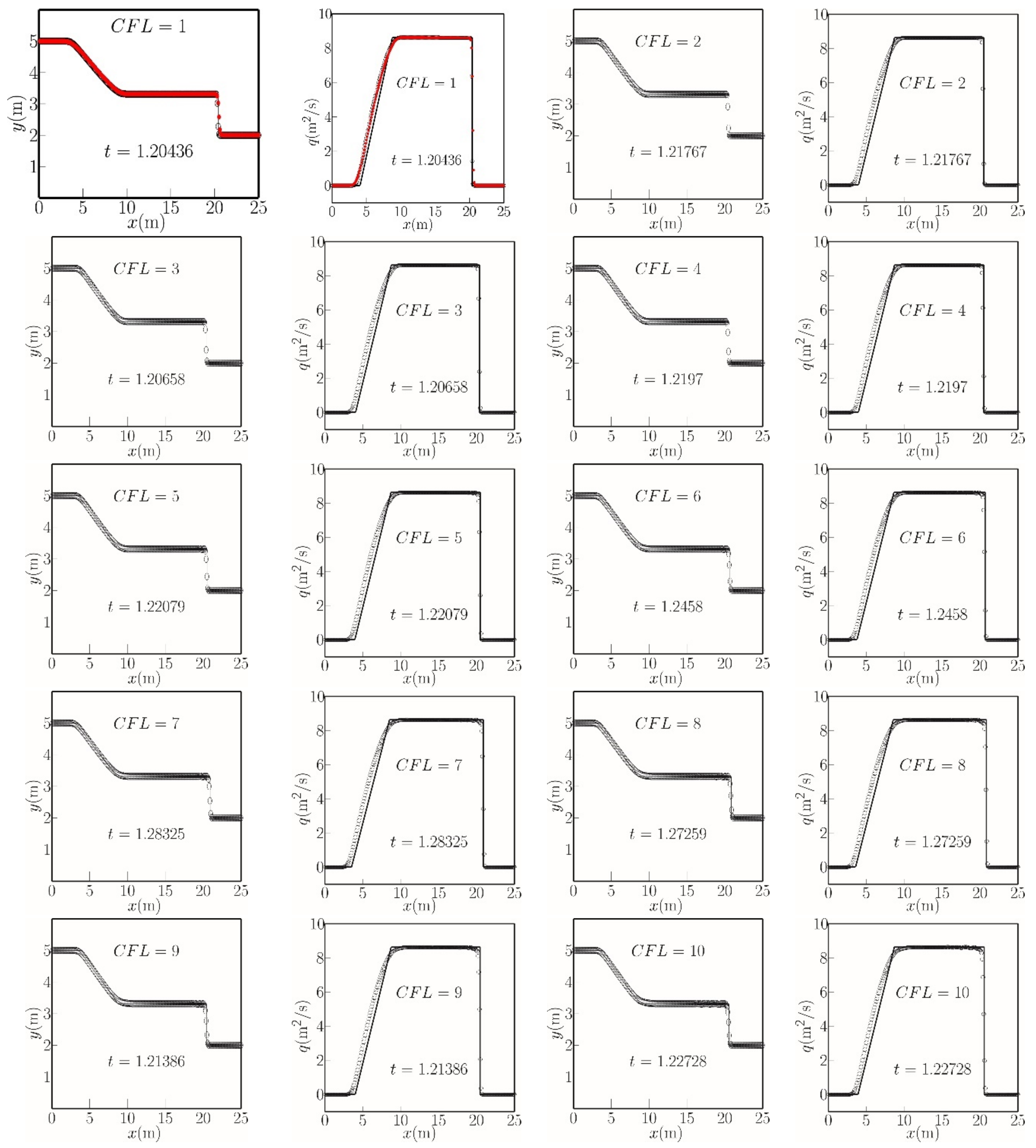
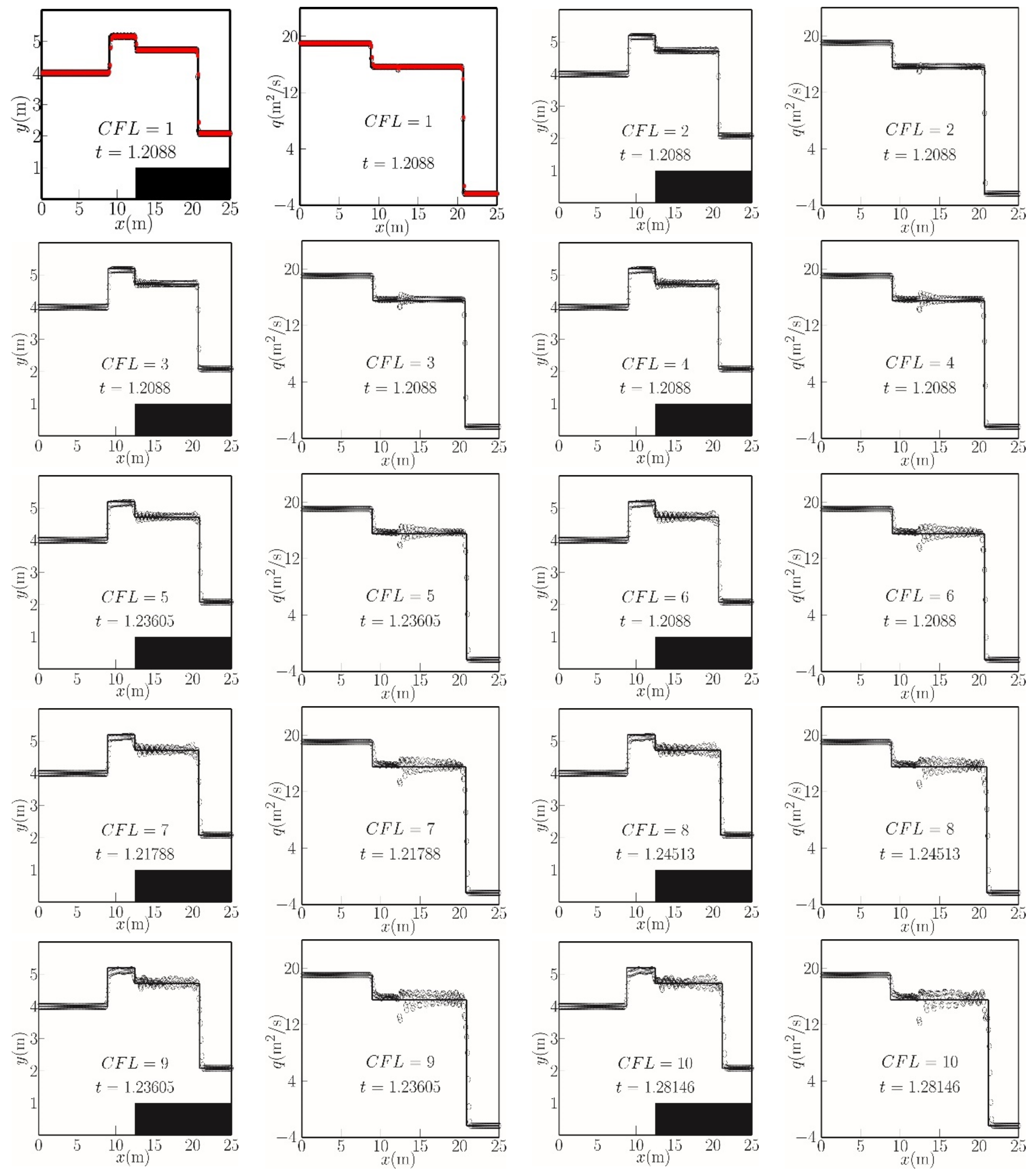
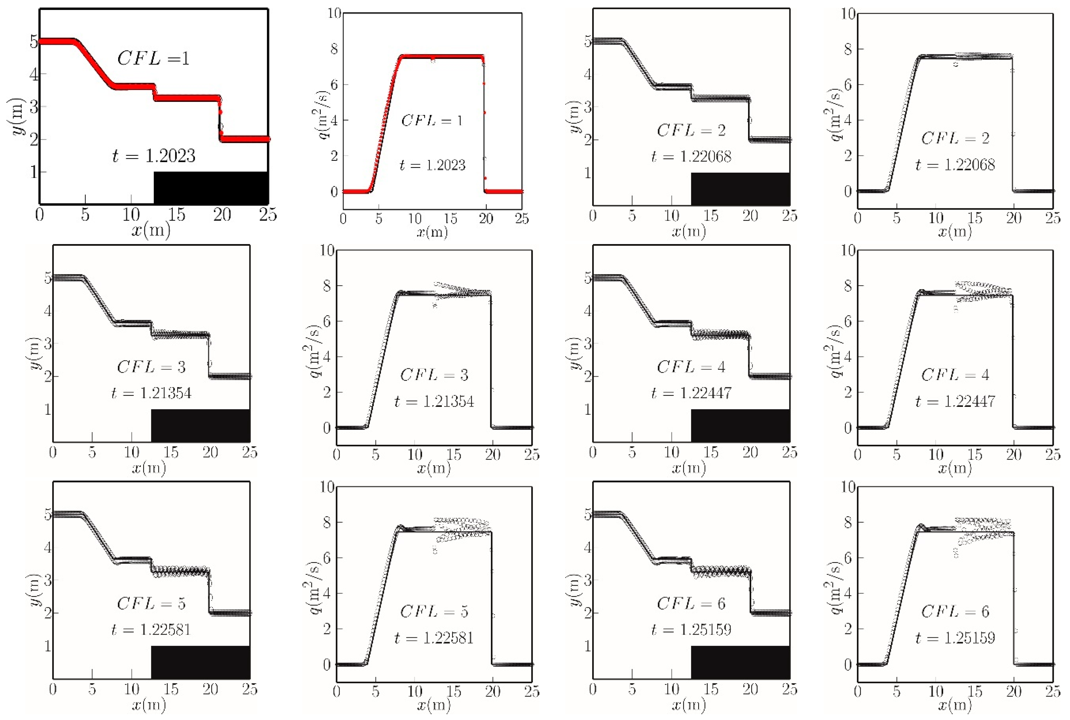
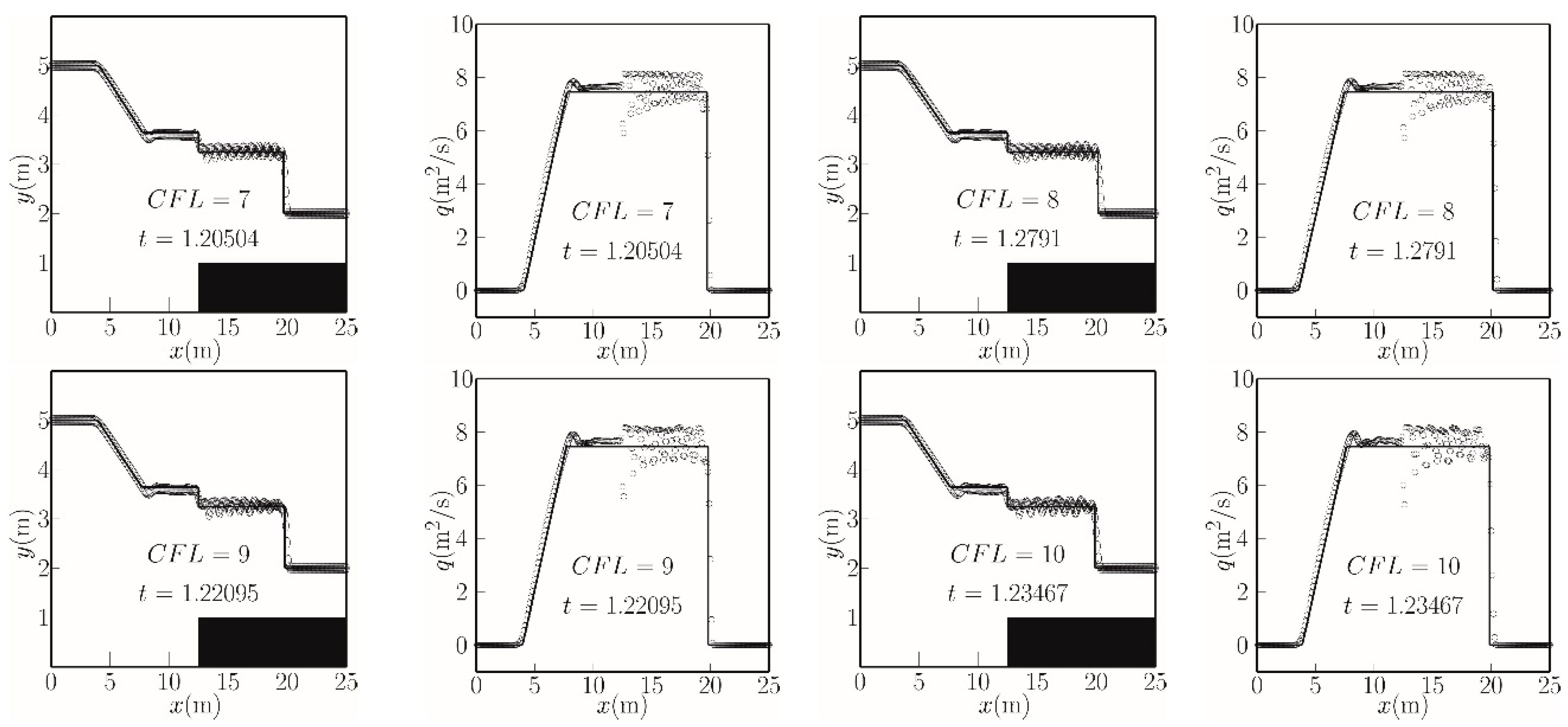
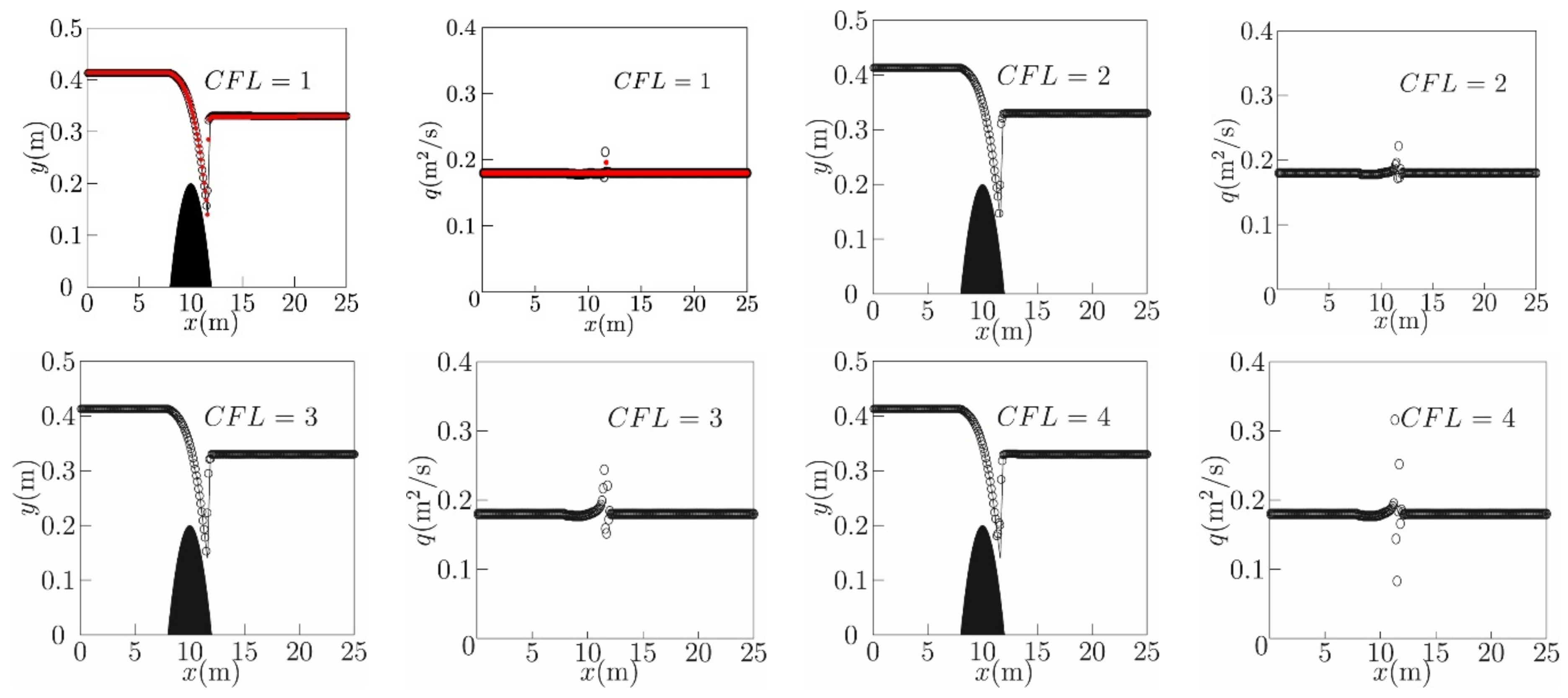
This paper applies TVD-LTS to solving the SWEs without viscous stresses and expands the scheme to non-homogeneous hyperbolic systems for the first time, to the authors’ knowledge. The results indicate that TVD-LTS gives a satisfactory representation of benchmark flows while suppressing spurious oscillations when solving homogeneous SWEs but is not as successful when applied to non-homogeneous SWEs. The paper has the following structure. Section 2 outlines the TVD-LTS solver of the shallow water equations. Section 3 presents results for different benchmark tests: homogeneous cases of two rarefactions; two shock waves; a single rarefaction and a shock wave; non-homogeneous cases of two rarefactions over a step; two shockwaves over a step; a single rarefaction and a bore over a step; and a transcritical flow over a bed hump. Section 4 provides the concluding remarks.

2. TVD-LTS Scheme

2.1. TVD-LTS Scheme for Scalar Case

Consider the homogeneous hyperbolic equation:

$$\frac{\partial u}{\partial t}+a\frac{\partial u}{\partial x}=0$$

(1)

Harten [16] proposed the following second order TVD-LTS scheme:

$$u_j^{n+1}=u_j^n-\lambda \left({\overline{f}}_{j+1/2}-{\overline{f}}_{j-1/2}\right)$$

(2)

where

$$\lambda {\overline{f}}_{j+1/2}=\frac{\lambda }{2}\left(f_j+f_{j+1}\right)+\frac{\lambda }{2}\left(g_j+g_{j+1}\right)-{\displaystyle \sum _{k=-K+1}^{K-1}{C}_k\left({\nu }_{j+k+1/2}+\gamma \right){\mathrm{\Delta }}_{j+k+1/2}{u}^n}$$

(3)

$$g_j^l=s_{j+1/2}\cdot \max \left\{0,\min \left({\sigma }_{j+1/2}\cdot \left|{\mathrm{\Delta }}_{j+1/2}u\right|, s_{j+1/2}\cdot {\sigma }_{j-1/2}\cdot {\mathrm{\Delta }}_{j-1/2}u\right)\right\}$$

(4)

$$\gamma =\frac{{\mathrm{\Delta }}_{j+1/2}g}{{\mathrm{\Delta }}_{j+1/2}u}$$

(5)

$$\nu =\frac{\lambda \mathrm{\Delta }t}{\mathrm{\Delta }x}$$

(6)

$$C_{\pm k}\left(\nu \right)=\left\{\begin{array}{l}{c}_k\left({\mu }_{\pm }\left(\nu \right)\right),1\le k\le K-1\hfill \\ \frac{K}{2}Q\left(\frac{\nu }{K}\right),k=0\hfill \end{array}\right.$$

(7)

$${\mu }_{\pm }\left(\nu \right)=\frac{1}{2}\left[Q\left(\frac{\nu }{K}\right)\pm \frac{\nu }{K}\right]$$

(8)

$$Q\left(\nu \right)=\left\{\begin{array}{ll}\frac{1}{2}\left(\frac{{\nu }^2}{\epsilon }+\epsilon \right),\hfill & \left|\nu \right|<\epsilon \hfill \\ \left|\epsilon \right|,\hfill & \left|\nu \right|\ge \epsilon \hfill \end{array}\right.$$

(9)

$$c_l\left(x\right)=\left\{\begin{array}{ll}-\left(\begin{array}{c}K\\ l\end{array}\right)x^l{\displaystyle \sum _{k=1}^{K-l}\left(\begin{array}{c}K-l\\ k\end{array}\right)}\frac{kl}{\left(k+l-1\right)\left(k+l\right)},\hfill & l\ge 1\hfill \\ \frac{K}{2}x,\hfill & l=0\hfill \end{array}\right.$$

(10)

$${\mathrm{\Delta }}_{j+1/2}\left(\right)={\left(\right)}_{j+1}-{\left(\right)}_j$$

(11)

$${\sigma }_{j+1/2}^l=\sigma \left({\nu }_{j+1/2}^l\right)=\frac{K}{2}\left\{Q\left(\frac{{\nu }_{j+1/2}^l}{K}\right)\left[1+\frac{K-1}{2}Q\left(\frac{{\nu }_{j+1/2}^l}{K}\right)\right]-\frac{K+1}{2}{\left(\frac{{\nu }_{j+1/2}^l}{K}\right)}^2\right\}$$

(12)

Now, we consider the non-homogeneous case:

$$\frac{\partial u}{\partial t}+a\frac{\partial u}{\partial x}=\frac{\partial s\left(x\right)}{\partial x}$$

(13)

The equation is discretized with the TVD-LTS method:

$$u_j^{n+1}=u_j^n-\lambda \left({\overline{f}}_{j+1/2}-{\overline{f}}_{j-1/2}\right)+\mathrm{\Delta }t\frac{\left(s_{j-1}-s_{j+1}\right)}{2\mathrm{\Delta }x}$$

(14)

According to Harten’s TVD-LTS scheme, $C_k\left(x\right)$ in Equation (3) is a Lipschitz continuous function, and so:

$$\left|\left[C_k\left({\nu }_{i+1/2}+{\gamma }_{i+1/2}\right)-C_k\left({\nu }_{i+1/2}\right)\right]{\mathrm{\Delta }}_{i+1/2}u\right|\le K\left|{\gamma }_{i+1/2}{\mathrm{\Delta }}_{i+1/2}u\right|=O\left(\mathrm{\Delta }{x}^2\right)$$

(15)

Therefore,

$$\begin{array}{ll}\left|C_k\left({\nu }_{j+k+1/2}+{\gamma }_{j+k+1/2}\right){\mathrm{\Delta }}_{j+k+1/2}u\right|& =C_k\left({\nu }_{j+k+1/2}\right){\mathrm{\Delta }}_{j+k+1/2}u+O\left(\mathrm{\Delta }{x}^2\right)\\ & =C_k\left(\nu \right)\mathrm{\Delta }x{u}_{x_{\left|j+k+1/2\right.}}+O\left(\mathrm{\Delta }{x}^2\right)\\ & =\mathrm{\Delta }x{C}_k\left(\nu \right)u_{x_{\left|j+k+1/2\right.}}+O\left(h^2\right)\end{array}$$

(16)

Substituting into Equation (3), and we obtain:

$$\lambda {\overline{f}}_{i+1/2}={\left[\lambda f+\mathrm{\Delta }x\sigma \left(\nu \right)u_x-\mathrm{\Delta }x{\displaystyle \sum _{k=-K+1}^{K-1}{C}_k\left(\nu \right)u_x}\right]}_{j+1/2}+O\left(\mathrm{\Delta }{x}^2\right)$$

(17)

Given

$${\displaystyle \sum _{k=-K+1}^{K-1}{C}_k\left(\nu \right)=\frac{1}{2}}Q\left(\nu \right)+\frac{1}{2}K\left(K-1\right)\left\{{\left(\frac{1}{2K}\left[Q\left(\nu \right)-\nu \right]\right)}^2-{\left(\frac{1}{2K}\left[Q\left(\nu \right)+\nu \right]\right)}^2\right\}$$

(18)

Equation (17) becomes:

$$\lambda {\overline{f}}_{i+1/2}={\left[\lambda f-\frac{1}{2}\mathrm{\Delta }x{\nu }^2{u}_x\right]}_{j+1/2}+O\left(\mathrm{\Delta }{x}^2\right)$$

(19)

The first part of Equation (14) is second order. The remaining part,

$$\frac{\partial s\left(x\right)}{\partial x}=\frac{\left(s_{j-1}-s_{j+1}\right)}{2\mathrm{\Delta }x},$$

(20)

is also second order in space, and so Equation (14) is entirely second order in space.

The source term is solely a function of space and will not change in time, and so it will not change the property of total variation diminishing, as verified by Harten [16]. Then, it is stable.

2.2. TVD-LTS Scheme for Shallow Water Equations

We consider shallow free surface flows in the horizontal dimension and assume hydrostatic pressure. The resulting inviscid shallow water equations (see, e.g., [2]) in the general matrix-vector form are expressed as:

$$\frac{\partial \mathit{U}}{\partial t}+\frac{\partial \mathit{F}\left(\mathit{U}\right)}{\partial x}={\mathit{S}}_f$$

(21)

For the homogeneous condition (with no bed slope), the vectors of dependent variables, horizontal fluxes, and source terms are:

$$\mathit{U}=\left[\begin{array}{c}h\\ hu\end{array}\right],\mathit{F}\left(\mathit{U}\right)=\left[\begin{array}{c}hu\\ h{u}^2+\frac{1}{2}g{h}^2\end{array}\right],{\mathit{S}}_f=\left[\begin{array}{c}0\\ 0\end{array}\right]$$

(22)

For the non-homogeneous condition with a finite bed slope, the vectors become [22]:

$$\mathit{U}=\left[\begin{array}{c}\eta \\ hu\end{array}\right],\mathit{F}\left(\mathit{U}\right)=\left[\begin{array}{c}hu\\ h{u}^2+\frac{1}{2}g\left({\eta }^2-2\eta z\right)\end{array}\right],{\mathit{S}}_f=\left[\begin{array}{c}0\\ -g\eta \frac{\partial z}{\partial x}\end{array}\right]$$

(23)

In Equations (21)–(23), U is the vector of stage and discharge, F(U) is the vector of horizontal fluxes, S_f is the vector of source terms, x is distance, t is time, h is the local water depth, u is mean flow velocity, g is the acceleration due to gravity, η is the stage (i.e., water free surface elevation above a fixed horizontal datum), and z is the bed elevation above the same datum.

In Roe’s method, the dependent variables at adjacent cells j and j + 1 are averaged as:

$$\tilde{c}=\sqrt{\frac{g{h}_j+g{h}_{j+1}}{2}}, \tilde{u}=\frac{u_j\sqrt{h_j}+u_{j+1}\sqrt{h_{j+1}}}{\sqrt{h_j}+\sqrt{h_{j+1}}}$$

(24)

Equation (21) describes a nonlinear hyperbolic system for which the Jacobi matrix can be written:

$$\mathit{A}=\frac{\partial \mathit{F}}{\partial \mathit{U}}=\left[\begin{array}{cc}0& 1\\ {\tilde{c}}^2-{\tilde{u}}^2& 2\tilde{u}\end{array}\right]$$

(25)

After diagonalization:

$$\mathit{A}=\mathit{L}\mathit{\Lambda }\mathit{R}=\frac{1}{{\lambda }^2-{\lambda }^1}\left[\begin{array}{cc}{\lambda }^2& -1\\ -{\lambda }^1& 1\end{array}\right]\left[\begin{array}{cc}{\lambda }^1& 0\\ 0& {\lambda }^2\end{array}\right]\left[\begin{array}{cc}1& 1\\ {\lambda }^1& {\lambda }^2\end{array}\right]$$

(26)

where the characteristic eigenvalues are:

$$\left\{\begin{array}{c}{\lambda }^1=\tilde{u}-\tilde{c}\\ {\lambda }^2=\tilde{u}+\tilde{c}\end{array}\right.$$

(27)

The vector difference in $\mathit{U}$ between adjacent cells is transferred to the characteristic space, such that:

$${\mathrm{\Delta }}_{j+1/2}\mathit{U}={\mathit{U}}_{j+1}-{\mathit{U}}_j={\left[\begin{array}{c}h\\ hu\end{array}\right]}_{j+1}-{\left[\begin{array}{c}h\\ hu\end{array}\right]}_j=\left[\begin{array}{c}{\alpha }^1\\ {\alpha }^2\end{array}\right]\mathit{R}$$

(28)

$$\left[\begin{array}{c}{\alpha }^1\\ {\alpha }^2\end{array}\right]=\left[\begin{array}{c}\frac{\left(\tilde{c}+\tilde{u}\right){\mathrm{\Delta }}_{j+1/2}h-{\mathrm{\Delta }}_{j+1/2}\left(hu\right)}{2\tilde{c}}\\ \frac{\left(\tilde{c}-\tilde{u}\right){\mathrm{\Delta }}_{j+1/2}h+{\mathrm{\Delta }}_{j+1/2}\left(hu\right)}{2\tilde{c}}\end{array}\right]$$

(29)

Equation (21) is then differenced using an explicit upwind scheme to give:

$${\mathit{U}}_j^{n+1}={\mathit{U}}_j^n-\frac{\mathrm{\Delta }t}{\mathrm{\Delta }x}\left({\widehat{\mathit{F}}}_{j+1/2}-{\widehat{\mathit{F}}}_{j-1/2}\right)-\frac{\mathrm{\Delta }t}{2\mathrm{\Delta }x}g\eta \left(z_{j-1}-z_{j+1}\right)$$

(30)

Following Harten [16], the numerical flux in TVD-LTS is:

$$\begin{array}{l}{\widehat{\mathit{F}}}_{j+1/2}=\frac{1}{2}\left({\mathit{F}}_j+{\mathit{F}}_{j+1}\right)+\frac{\mathrm{\Delta }x}{2\mathrm{\Delta }t}{\displaystyle \sum _{l=1}^m{R}_{j+1/2}^l\left(g_j^l+g_{j+1}^l\right)}\\ \begin{array}{ccc}\begin{array}{cc}& \end{array}& & \end{array}-\frac{\mathrm{\Delta }x}{\mathrm{\Delta }t}{\displaystyle \sum _{k=-K+1}^{K-1}\left[{\displaystyle \sum _{l=1}^m{C}_k{\left({\nu }^l+{\gamma }^l\right)}_{j+k+1/2}{\alpha }_{j+k-1/2}^l}\right]}\end{array}$$

(31)

where

$$g_j^l=s_{j+1/2}\cdot \max \left\{0,\min \left({\sigma }_{j+1/2}^l\cdot \left|{\alpha }_{j+1/2}^l\right|, s_{j+1/2}\cdot {\sigma }_{j-1/2}^l\cdot {\alpha }_{j-1/2}^l\right)\right\}$$

(32)

$${\gamma }_{j+1/2}^l=\left\{\begin{array}{cc}\frac{{\mathrm{\Delta }}_{j+1/2}{g}^l}{{\alpha }_{j+1/2}^l},& {\alpha }_{j+1/2}^l\ne 0\\ 0,& {\alpha }_{j+1/2}^l=0\end{array}\right.$$

(33)

$$s_{j+1/2}=\mathrm{sgn}\left({\alpha }_{j+1/2}^l\right)$$

(34)

Equations (7)–(9) ensure that each grid cell is correctly allocated to the right interface waves ($k>0$) when they spread to the left ($\nu <0$) and to the left interface waves ($k<0$) when they spread to the right ($\nu >0$).

3. Results

3.1. Homogeneous SWEs

The numerical model is tested against three benchmark cases involving different combinations of rarefaction and shock waves propagating in a frictionless, straight, 25 m long one-dimensional channel with a fixed horizontal bed, for which exact solutions are provided by Toro [2]. The domain is discretized into 250 cells, such that ∆x = 0.1 m. The adaptive time step is determined from ∆t = K ∆x/λ_max, where K is the CFL number, and λ_max is the maximum eigenvalue in Equation (27). The initial time step is 0.01 s, after which its value depends on the instantaneous value of λ_max. Throughout the computations, the local flow depth and velocity are updated using Equation (30), in which the final term is set to zero for the flat bed.

3.1.1. Two Rarefaction Waves in a Horizontal Channel

We first consider a case of diverging flow, when the channel initially carries an upstream flow of mean velocity −2 m/s and depth 8.0 m for x < 12.5 m and a downstream flow of mean velocity 7.1704 m/s and depth 5.0 m for x ≥ 12.5 m. Table 1 provides a brief summary of the initial conditions.

Table 1. Initial conditions for a homogeneous case of two rarefaction waves in a frictionless, horizontal channel.

	h (m)	q (m2/s)
Left side (x < 12.5 m)	8.0	−16.0
Right side (x ≥ 12.5 m)	5.0	35.852

Figure 1 presents the distributions of the water free surface and discharge per unit width along the channel for different CFL numbers using the present TVD-LTS model. In Figure 1, the upper-left plots display the distributions obtained for a maximum CFL of unity at time t = 0.70158 s. The predicted water free surface profiles provide a satisfactory match to the solution by Toro’s method [2] and Roe’s scheme [3], with the head of the leftward rarefaction wave occurring at x = 4.0 m and its tail at x = 12 m and the head of the rightward rarefaction wave at x = 16 m and its tail at x = 22.4 m. The computed and exact mass flux distributions are very similar, except for the slight deviation at the interface between the flow plateau and the rarefaction.

Figure 1. Free surface and mass flux profiles for two rarefaction waves in a frictionless, horizontal channel at a given time instant. Toro’s [2] almost exact solution (solid lines), Roe’s [3] scheme (red circles), and TVD-LTS predictions (open circles) for CFL = 1 to 10.

3.1.2. Two Shockwaves in a Horizontal Channel

Next, we consider an idealized hydraulic bore caused by a tide interacting with an opposing river flow in the horizontal channel. The initial conditions listed in Table 2 consist of a right-directed initial flow at a speed of 5.75 m/s in water depth of 4 m and a left-directed flow at a speed of 5.1854 m/s in water depth of 1.0838 m.

Table 2. Initial conditions for a homogeneous case of two shockwaves in a frictionless, horizontal channel.

	h (m)	q (m2/s)
Left side (x < 12.5 m)	4.0	23
Right side (x ≥ 12.5 m)	1.0838	−5.6199

Figure 2 shows the water free surface and mass flux distributions along the channel, predicted by the TVD-LTS model for different CFL numbers. There is generally close agreement with Toro’s [2] exact solution. In Figure 2, the profiles correspond to a right-directed hydraulic bore at x = 17.2 m and a left-directed hydraulic bore at x = 10.6 m. The upper-left plots display the results obtained for a maximum CFL value of unity. Oscillations in the TVD-LTS solution become increasingly evident as the CFL number becomes larger.

Figure 2. Free surface and mass flux profiles for two shockwaves in a frictionless, horizontal channel at a given time instant. Toro’s [2] almost exact solution (solid lines), Roe’s [3] scheme (red circles), and TVD-LTS predictions (open circles) for CFL = 1 to 10.

3.1.3. One Rarefaction and One Shockwave in a Horizontal Channel

The third case involves a dam break over a wet bed that is initially quiescent. The initial conditions are summarized in Table 3.

Table 3. Initial conditions for a homogeneous case of one rarefaction and one hydraulic bore in a frictionless, horizontal channel.

	h (m)	q (m2/s)
Left side (x < 12.5 m)	5.0	0
Right side (x ≥ 12.5 m)	2.0	0

Figure 3 presents the computed water free surface and mass flux distributions along the channel for different CFL numbers. Here, the exact solution obtained by Toro [2] consists of a right-directed hydraulic bore at x = 20.2 m and a left-directed rarefaction wave, whose head is at x = 2.4 m and tail is at x = 9.9 m. Again, we can see that the predicted distributions provide a reasonable match to the exact solution when CFL is unity. As the CFL number increases, slight oscillations become noticeable at the location between the flat free surface and the shock wave.

Figure 3. Free surface and mass flux profiles for one rarefaction and one shock in a frictionless, horizontal channel at a given time instant. Toro’s [2] almost exact solution (solid lines), Roe’s [3] scheme (red circle), and TVD-LTS predictions (open circles) for CFL = 1 to 10.

3.2. Non-Homogeneous SWEs

The next three cases concern the propagation of rarefactions and shocks over an abrupt step in the bed (i.e., a shelf), where the SWEs become non-homogeneous owing to the presence of bed slope terms. In the Godunov-type FVM scheme, each interface between cells is considered as a discontinuity that can only be solved by a Riemann solver, and so these cases (such as the bed step) are benchmark foundations from which the method can be extended to more practical problems. For example, local discontinuities are likely to occur when a continuous river bed is discretized. Exact solutions for the three benchmark cases are given by Rosatti and Begnudelli [23]. The final case considers a transcritical flow at a bed hump, again where the SWEs are non-homogeneous, for which an exact solution is given by Goutal and Maurel [24]. In all cases, the channel has an overall length of 25 m, a constant spatial increment of ∆x = 0.1 m, and an initial time step of 0.01 s (which is altered at every time step thereafter, according to ∆t = K ∆x/λ_max). The flow depth and velocity are updated using Equation (30), but with the final term no longer zero at the step.

3.2.1. Two Rarefaction Waves in a Channel Containing a Bed Step

The first test case considers flow in a channel containing a 1 m high abrupt step, with the bed elevation defined as z = 0 for x < 12.5 m and z = 1 m for x ≥ 12.5 m. For diverging flow, the initial depth either side of the shelf is 8.0 and 5.0 m, with corresponding opposing velocities of −2 and 7.1704 m/s (Table 4).

Table 4. Initial conditions for two rarefaction waves propagating over a step.

	h (m)	q (m2/s)	z (m)
Left side (x < 12.5 m)	8.0	−16.0	0
Right side (x ≥ 12.5 m)	5.0	35.852	1

Figure 4 shows the computed and exact solutions for the water free surface and discharge per unit width distributions, obtained using different CFL numbers. In all cases, the free surface profiles consistently contain a left-directed rarefaction wave whose head is at x = 3.1 m and tail is at x = 10 m. A stationary shock occurs at the step. Additionally, a right-directed rarefaction wave is evident, with its head at x = 19 m and its tail at x = 22.4 m. The computed and exact mass flux distributions are in satisfactory agreement, except for a slight oscillation at the interface of the step (x = 12.5 m) in the mass flux from CFL number 1 to CFL number 10.

Figure 4. Free surface and mass flux profiles for two rarefaction waves in a channel containing a bed step at a given time instant. Rosatti and Begnudelli [23]’s analytical solution (solid lines), well-balanced scheme [22] (red circles), and TVD-LTS predictions (open circles) for CFL = 1 to 10. The solid rectangle indicates the bed shelf.

3.2.2. Two Shockwaves in a Channel Containing a Bed Step

The second test case considers an idealized upstream-propagating tidal bore interacting with a downstream-propagating river flow in the same channel as in the previous case. The upstream depth to the left of the bore is 4.0 m, and the velocity is 4.75 m/s. The downstream depth to the right of the bore is 1.0838 m on top of a 1 m elevated riverbed so that the stage is 2.0838 m and the flow velocity is −2.1854 m/s. Here, the opposing bore and river flows approach the middle interface in opposite directions (Table 5).

Table 5. Initial conditions for two hydraulic shocks (bores) propagating over a step.

	h (m)	q (m2/s)	z (m)
Left side	4.0	19	0
Right side	1.0838	−2.3685	1

Figure 5 shows the computed and analytical solutions for the water free surface and mass flux distributions along the channel, obtained for different CFL numbers. The solution again includes a stationary shock at the front edge of the shelf but is different from the preceding case in that the waves emanating from either side are no longer rarefactions but, instead, are two bores at x = 8 m and x = 21 m, traveling in opposite directions. In the TVD-LTS predictions, tiny oscillations in the mass flux can be discerned at the step (x = 12.5 m) even when the CFL number is only 1. At higher CFL numbers, the oscillations extend progressively to the right of the step (x > 12.5 m), with both the free surface and mass flux exhibiting increasingly intense fluctuations. Oscillations of relatively smaller amplitude also occur to the left of the step (x < 12.5 m).

Figure 5. Free surface and mass flux profiles for two shocks in a channel containing a bed step at a given time instant. Rosatti and Begnudelli [23]’s analytical solution (solid lines), well-balanced scheme [22] (red circles), and TVD-LTS predictions (open circles) for CFL = 1 to 10. The solid rectangle indicates the bed shelf.

3.2.3. One Rarefaction and One Shockwave in a Channel Containing a Bed Step

Unlike the previous two cases, this case involves zero flow velocity on either side of the step interface, as indicated in Table 6. The initial depths are 5.0 and 1.0 m to the left and right of the step.

Table 6. Initial conditions for a rarefaction and a hydraulic bore propagating over a step.

	h (m)	q (m2/s)	z (m)
Left side	5.0	0	0
Right side	1.0	0	1

Figure 6 presents water free surface and mass flux distributions along the channel obtained for different CFL numbers. In this case, the solution consists of a hydraulic drop at the front face of the step, a right-directed hydraulic bore at x = 20.3 m, and a left-directed rarefaction wave with its head at x = 2.8 m and its tail at x = 8.3 m. The predicted results to the left of the step face (i.e., x < 12.5 m) are better simulated than to the right of the step face, especially for larger values of the CFL number, with small amplitude oscillations occurring at the interface between the rarefaction and the flow plateau. The predicted mass flux at the step face (x = 12.5 m) is lower than the analytical result, even when the CFL number is only 1. Decaying fluctuations in the predicted results occur to the right of the front face of the step (x > 12.5 m), with the amplitude increasing with the CFL number. At the step face itself, the deviation between the predicted and analytical mass flux is at a maximum, independent of the CFL number considered (in the range from 1 to 10).

Figure 6. Free surface and mass flux profiles for a single rarefaction and a single shock in a channel containing a bed step at a given time instant. Rosatti and Begnudelli [23]’s analytical solution (solid lines), well-balanced scheme [22] (red circles), and TVD-LTS predictions (open circles) for CFL = 1 to 10. The solid rectangle indicates the bed shelf.

3.2.4. Transcritical Flow at a Fixed Bed Hump

Goutal and Maurel [24] derived the analytical solution for shallow flow over a hump in the riverbed where the bed level satisfies the following equation:

$$\left\{\begin{array}{ll}z=0.2-0.05{\left(x-10\right)}^2,\hfill & 8<x\le 12\hfill \\ z=0,\hfill & \mathrm{otherwise}\hfill \end{array}\right.$$

(35)

In this case, the channel is 25 m long and carries an upstream inlet discharge of 0.18 m³/s. The downstream outlet water level is prescribed to be 0.33 m. Initially, the water level is 0.33 m (see Figure 7). Figure 8 shows the analytical solution at a steady state. In the numerical model, the channel is divided into a regular grid of 250 cells, each with a spatial increment of x = 0.1 m. The initial time step is prescribed a value of 0.01 s, which alters each time step thereafter, according to ∆t = K ∆x/λ_max.

Figure 7. Bed elevation and initial water free surface distributions along a channel for the case of transcritical flow over a bed hump.

Figure 8. Analytical steady-state free surface elevation distribution [24] along a channel for the case of transcritical flow over a bed hump.

Figure 9 compares the numerical predictions of the water level and mass flux profiles obtained using Equation (30) against the analytical solution. Reasonable agreement is obtained between the predicted and analytical profiles when the CFL number is 1, 2, 3, and 4, but a converged solution cannot be obtained when the CFL number is larger than 4. The over-prediction of mass flux arises for CFL numbers 1 and 2. Over- and under-predictions are both observed for CFL numbers 3 and 4.

Figure 9. Analytical solution [24] (thin solid line), well-balanced scheme [22] (red circles), and LTS predictions using Algorithm 2 (open circles) of steady-state free surface elevation and mass flux distributions along a channel for transcritical flow at a fixed bed hump.

To investigate the efficiency of the TVD-LTS algorithm, the computational time overhead was determined. All computations were undertaken on the same computer, which was configured as follows: Intel Core i9-10900K @ 3.70 GHz with an overclock CPU; Kingston DDR4 128 GB 3200 MHz with XMP opened memory; and Intel 750 series PCIe interface 1.2 TB SSD (also used by the authors in their previous work [25]). Table 7 summarizes the computation effort in terms of the number of computational steps, CPU time, and average run time per computational step (determined as the ratio of CPU time to the number of steps) required for convergence to a steady state (difference of U between two neighboring time steps less than 10⁻⁵) for transcritical flow at a hump according to CFL number. It should be noted that the use of the same algorithm on the above computer could lead to slightly different CPU time evaluations because of the auto-arrangement of the CPU load and the use of random memory blocks. In all the tests considered, the discrepancy is in the range of ±0.2 s. The average run time per computational step is 5.73 × 10⁻³ s for a CFL number equal to 1. The run time increases to 31.64 × 10³ s when the CFL number is raised to 4. Unlike the first-order LTS scheme, the TVD-LTS accounts for information from all relevant cells even when their contribution is very small, thus complicating the coefficient (Equation (15)) and leading to an abrupt increase in calculation effort.

Table 7. Computational effort by a Godunov-type LTS solver compared to Roe’s scheme for different CFL numbers.

CFL Number	1	2	3	4	Roe
Steps	4338	2851	2338	1819	6099
CPU Time (s)	24.86	32.54	46.63	57.55	3.01
Time/Step (10−3 s)	5.73	11.41	19.94	31.64	0.49

4. Conclusions

Total variation diminishing (TVD) high order large time step schemes have been described for solving homogeneous and non-homogeneous versions of shallow water equations (SWEs), the latter containing bed slope source terms. The resulting model was tested extensively against standard benchmark tests for which standard solutions are available: three tests concerning discontinuous flow in a horizontal channel, three tests of discontinuous flow in a channel with a bed shelf, and one test of transcritical flow at a bed hump. In the first six cases, spurious oscillations develop as the CFL number increases and are most pronounced immediately downstream of the step when it is present. Rarefactions are properly simulated in all cases except for the under-prediction of mass flux at the step interface (x = 12.5 m). In general, the results for the homogeneous SWEs are better predicted than for the non-homogenous SWEs. For transcritical flow at a hump, satisfactory predictions were achieved for CFL numbers up to 4, beyond which the mass flux became overwhelmed by oscillations. The CPU time per simulation time step was found to be much larger than for the conventional first-order Roe scheme, and it increased progressively with increasing CFL number because information from more grid cells had to be accommodated at each time step. In practice, we found that the TVD-LTS scheme required fewer steps but at the cost of greater total computational time, indicating that high order LTS is not economical from a computational perspective.

References

- Abbott, M.B. Computational Hydraulics; Routledge: London, UK; New York, NY, USA, 1979; p. 324. [Google Scholar]
- Toro, E.F. Shock-Capturing Methods for Free-Surface Shallow Flows; John Wiley and Sons: New York, NY, USA, 2001. [Google Scholar]
- Roe, P.L. Approximate Riemann Solvers, Parameter Vectors, and Difference Schemes. J. Comput. Phys. 1981, 135, 250–258. [Google Scholar] [CrossRef]
- Osher, S.; Solomon, F. Upwind Difference Schemes for Hyperbolic Systems of Conservation Laws. Math. Comput. 1982, 38, 339–374. [Google Scholar] [CrossRef]
- Liou, M.; Steffen, C.J. A New Flux Splitting Scheme. J. Comput. Phys. 1993, 107, 23–39. [Google Scholar] [CrossRef]
- Shu, C.; Osher, S. Efficient implementation of essentially non-oscillatory shock-capturing schemes. J. Comput. Phys. 1988, 77, 439–471. [Google Scholar] [CrossRef]
- Shu, C.; Osher, S. Efficient implementation of essentially non-oscillatory shock-capturing schemes, II. J. Comput. Phys. 1989, 83, 32–78. [Google Scholar] [CrossRef]
- Leveque, R.J. Large Time Step Shock-Capturing Techniques for Scalar Conservation Laws. SIAM J. Numer. Anal. 1982, 19, 1091–1109. [Google Scholar] [CrossRef]
- Leveque, R.J. A Large Time Step Generalization of Godunov’s Method for Systems of Conservation Laws. SIAM J. Numer. Anal. 1985, 22, 1051–1073. [Google Scholar] [CrossRef]
- Murillo, J.; García-Navarro, P.; Brufau, P.; Burguete, J. Extension of an explicit finite volume method to large time steps (CFL > 1): Application to shallow water flows. Int. J. Numer. Methods Fluids 2006, 50, 63–102. [Google Scholar] [CrossRef]
- Morales-Hernández, M.; Murillo, J. A large time step 1D upwind explicit scheme (CFL > 1): Application to shallow water equations. J. Comput. Phys. 2012, 231, 6532–6557. [Google Scholar] [CrossRef]
- Morales-Hernández, M.; Hubbard, M.E.; García-Navarro, P. A 2D extension of a Large Time Step explicit scheme (CFL > 1) for unsteady problems with wet/dry boundaries. J. Comput. Phys. 2014, 263, 303–327. [Google Scholar] [CrossRef]
- Morales-Hernández, M.; Lacasta, A.; Murillo, J.; García-Navarro, P. A Large Time Step explicit scheme (CFL > 1) on unstructured grids for 2D conservation laws: Application to the homogeneous shallow water equations. Appl. Math. Model. 2017, 47, 294–317. [Google Scholar] [CrossRef]
- Qian, Z.; Lee, C. A class of large time step Godunov schemes for hyperbolic conservation laws and applications. J. Comput. Phys. 2011, 230, 7418–7440. [Google Scholar] [CrossRef]
- Harten, A. High resolution schemes for hyperbolic conservation laws. J. Comput. Phys. 1983, 49, 357–393. [Google Scholar] [CrossRef]
- Harten, A. On a Large Time-Step High Resolution scheme. Math. Comput. 1986, 46, 379–399. [Google Scholar] [CrossRef]
- Qian, Z.; Lee, C. On large time step TVD scheme for hyperbolic conservation laws and its efficiency evaluation. J. Comput. Phys. 2012, 231, 7415–7430. [Google Scholar] [CrossRef]
- LeVeque, R.J. Balancing Source Terms and Flux Gradients in High-Resolution Godunov Methods: The Quasi-Steady Wave-Propagation Algorithm. J. Comput. Phys. 1998, 146, 346–365. [Google Scholar] [CrossRef]
- Hubbard, M.E.; Garcia-Navarro, P. Flux Difference Splitting and the Balancing of Source Terms and Flux Gradients. J. Comput. Phys. 2000, 165, 89–125. [Google Scholar] [CrossRef]
- Zhou, J.G.; Causon, D.; Mingham, C.; Ingram, D. The Surface Gradient Method for the Treatment of Source Terms in the Shallow-Water Equations. J. Comput. Phys. 2001, 168, 1–25. [Google Scholar] [CrossRef]
- Rogers, B.D.; Borthwick, A.G.L.; Taylor, P.H. Mathematical balancing of flux gradient and source terms prior to using Roe’s approximate Riemann solver. J. Comput. Phys. 2003, 192, 422–451. [Google Scholar] [CrossRef]
- Liang, Q.; Borthwick, A.G.L. Adaptive quadtree simulation of shallow flows with wet-dry fronts over complex topography. Comput. Fluids 2009, 38, 221–234. [Google Scholar] [CrossRef]
- Rosatti, G.; Begnudelli, L. The Riemann Problem for the one-dimensional, free-surface Shallow Water Equations with a bed step: Theoretical analysis and numerical simulations. J. Comput. Phys. 2010, 229, 760–787. [Google Scholar] [CrossRef]
- Goutal, N.; Maurel, F. Proceedings of the 2nd Workshop on Dam-Break Wave Simulation; Department Laboratoire National d’Hydraulique, Groupe Hydraulique Fluviale: Toulouse, France, 1997. [Google Scholar]
- Xu, R.Y.; Borthwick, A.G.; Ma, H.; Xu, B. Godunov-type large time step scheme for shallow water equations with bed-slope source term. Comput. Fluids 2022, 233, 105222. [Google Scholar] [CrossRef]
Publisher’s Note: MDPI stays neutral with regard to jurisdictional claims in published maps and institutional affiliations. |
© 2022 by the authors. Licensee MDPI, Basel, Switzerland. This article is an open access article distributed under the terms and conditions of the Creative Commons Attribution (CC BY) license (https://creativecommons.org/licenses/by/4.0/).