The Characteristics of Nonlinear Trends and the Complexity of Hydroclimatic Change in China from 1951 to 2014

Abstract

Hydroclimatic change across China has received considerable attention due to its vital significance for regional ecosystem stability and economic development, yet the spatiotemporal dynamics of its nonlinear trends and complexity have not been fully understood. Herein, the spatiotemporal evolution of Dai’s self-calibrating Palmer drought severity index (scPDSI) trends in China during the period from 1951 to 2014 is diagnosed using the ensemble empirical mode decomposition (EEMD) method. A persistent and noticeable drying has been identified in North and Northeastern China (NNEC) since the 1950s. Significant wetting in the north of the Tibetan Plateau (TP) and the south of the western parts of Northwestern China (WNWC) started sporadically at first and accelerated until around 1980. A slight wetting trend was found in Southwest China (SC) before 1990, followed by the occurrence of a dramatic drying trend over the following decades. In addition, we have found that the scPDSI variations in WNWC and the TP are more complex than those in NNEC and SC based on our application of Higuchi’s fractal dimension (HFD) analysis, which may be related to complex circulation patterns and diverse geomorphic features.

1. Introduction

Due to the diverse effects of complex topography and multiple climate forcings [1], hydroclimatic variability in China can vary dramatically across time and space. Despite this, one common feature is that extreme drought can hit any region across China, where dramatic and persistent moisture fluctuations are often accompanied by catastrophic societal and economic consequences for millions of people [2,3,4]. For instance, the 1630s–1640s drought was widespread over North China, contributing to the demise of the Chinese Ming dynasty [5,6,7]. A widely documented drought occurred in the late 1920s over Northwest China, resulting in the death of at least 4 million people [8,9]. In addition, as was clearly shown by the occurrence of severe drought events in the autumn of 2009 over southwest China and in the autumn of 2009 over South China [10,11], humid, subtropical China is not immune to water shortages either. Therefore, investigations concerning the spatial and temporal patterns of hydroclimatic variability across China are highly necessary to a better understanding of the underlying climate forcings.

A large body of research has examined hydroclimatic variation trends in specific regions of China [12,13,14,15] or the entirety China [16,17,18,19]. However, the shape of the trend found by many of these studies was basically determined a priori (e.g., by straight-line fitting), which can only extract a constant rate of variability over a timespan. In fact, time-unvarying changes cannot effectively exhibit the hidden, nonstationary nature of a time series since climatic changes are often uniform on different spatial and temporal scales. To address this problem, recent works have started to reflect the nonlinear trends of climatic change by using the ensemble empirical mode decomposition (EEMD) method [20,21,22]. The definition of a trend in a time series in EEMD requires the removal of any identifiable oscillatory components and the retention of one extremum, at most, within a given data-span [23]. To date, no studies have provided a reasonable diagnosis of the evolution of hydroclimatic variability on the different spatiotemporal scales across the entirety of China based on EEMD.

Climate can be identified as a set of atmospheric states of a dynamic chaotic system with deterministic nonlinear variability [24]. Although they have become increasingly more complex and capable of providing fairly reliable predictions of future climatic developments, climate models still cannot cover all potential mechanisms, and the outputs always include considerable uncertainties, especially for large-scale simulations [25]. Therefore, the interpretation of climate as a complex intervariable organization is a key option for better understanding the spatiotemporal evolution of dynamic systems [26,27]. To date, many concepts (e.g., entropy, fractals, chaos) have been introduced to explain the complexity of climatic change processes [28,29,30], yet the extension of these studies is still limited. Plus, considering hydroclimatic change as attenuated by more frequent extremes under global warming, the way in which to understand the spatiotemporal complexity of the hydroclimatic system in China tends to be a key issue that needs to be investigated.

In this context, the objective of the present study is to explore the spatial and temporal evolution of the nonlinear tendency and the complexity of hydroclimatic change across China. Section 2 presents the data and the methods employed in this study. In Section 3, Section 4, and Section 5, we investigate the spatial distribution of the EEMD time-varying trends and the fractal dimension from multiple timescales of the scPDSI series in China, and we discuss the potential driving mechanisms for these variations. The major findings are given in Section 6.

2. Dataset and Methods

2.1. Dataset Description

The hydroclimatic index used herein is Dai’s self-calibrating Palmer drought severity index (scPDSI), with potential evapotranspiration estimated by using the more sophisticated Penman–Monteith equation based on historical data [31]. The scPDSI is calculated from a water-balance model forced by observed monthly precipitation and temperature, and it is calibrated by local climatic conditions instead of the fixed coefficients used by Palmer [32]. Thus, the scPDSI is more spatially comparable than is the original PDSI developed by [33]. We use an updated version of the scPDSI, with global coverage based on a 2.5° × 2.5° gridding system, spanning the years from 1850 to 2014 (http://www.cgd.ucar.edu/cas/catalog/climind/pdsi.html, accessed on 13 March 2016). Since most of the meteorological stations in China were not established until the 1950s, we only use the scPDSI for the period from 1951 to 2014 (a total of 768 months). A total of 193 scPDSI grid points across China are used in this study (Figure 1).

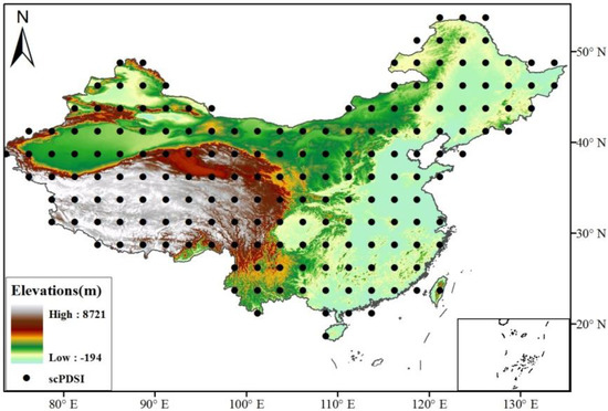
Figure 1. Map showing the locations of the gridded scPDSI across China. The scPDSI grid points were developed by Dai et al. (2011) for global coverage based on a 2.5° × 2.5° gridding system.

2.2. Ensemble Empirical Mode Decomposition

The original empirical mode decomposition method uses extrema information to separate the oscillations on different scales and the nonlinear trend from a time series [34], yet changes in extrema locations and values can easily result in different decompositions, leading totally different physical interpretations. The EEMD, a noise-assisted data-analysis method, is developed to improve the “mode mixing” problem [23]. In EEMD, a time series x(t) at a grid point is decomposed in terms of adaptively obtained, amplitude–frequency modulated oscillatory components Cj and a residual Rn, a curve either monotonic or containing only one extremum from which no additional oscillatory components can be extracted:

$$x\left(t\right)={\displaystyle \sum }_{j=1}^n{C}_j\left(t\right)+R_n\left(t\right)$$

(1)

The trend follows no a priori shape and changes over time after the intrinsic variability of various timescales is removed. It is also more sensitive to the extension of new data. The physical interpretation within specified time intervals does not vary with the addition of data, and the subsequent evolution of a physical system cannot also alter the reality of that which has already happened [23]. Based on the time-varying nature of the EEMD trend, we diagnose the variation at a given time (t) from a reference time of 1951:

$$Trend\left(t\right)=R_n\left(t\right)-R_n\left(1\right)$$

(2)

In addition, we also test the statistical significance of an EEMD trend at a given temporospatial location based on the Monte Carlo method introduced by Ji et al. [21].

2.3. Higuchi’s Fractal Dimension

An efficient algorithm for measuring the fractal dimension of a discrete signal directly in the time domain was proposed by [35]. This algorithm is simpler and faster than many other classical measures derived from chaos theory (e.g., correlation dimension) because the reconstruction of the attractor phase space is not essential [36]. Higuchi’s fractal dimension (HFD) has been widely employed to quantify the complexity and the self-similarity from a signal [37,38,39]. Its principle for computing the fractal dimension can be described in the following manner:

Given a one-dimensional time series X = {x(1), x(2), …, x(N)}, where N denotes the total number of samples, the algorithm that constructs k new time series $x_m^k$ is defined by:

$$x_m^k=\left\{x\left(m\right),x\left(m+k\right),\cdots ,x\left(m+\left[\frac{N-m}{k}\right]k\right)\right\}$$

(3)

where k and m are integers, [•] is the integer part of •, k indicates the discrete time interval between points, and $m=1, 2,\dots , k$ represents the initial time value. The length of each new time series can be calculated as:

$$L\left(m,k\right)=\frac{\left\{\left({{\displaystyle \sum }}_{i=1}^{\left[\left(N-m\right)/k\right]}\left|x\left(m+ik\right)-x\left(m+\left(i-1\right)k\right)\right|\right)\frac{N-1}{\left[\left(N-m\right)/k\right]k}\right\}}{k}$$

(4)

where N is the length of the original time series, and $\frac{N-1}{\left[\left(N-m\right)/k\right]k}$ is the normalization factor. The length of the series L(k) is obtained by averaging all of the subseries lengths L(m, k) that have been obtained for a given k value:

$$L\left(k\right)=\frac{1}{k}{\displaystyle \sum }_{m=1}^{k}L\left(m,k\right)$$

(5)

If $L\left(k\right)\propto k^{-D}$, that is, if it behaves as a power law, we regard the exponent D as the FD of the original series.

3. General Aspects of the scPDSI

The scPDSI values across China show a normal-like distribution (skewness = 0.028) with most values (79.3%) occurring at the near-normal conditions (−3 < scPDSI < 3), and the frequencies of the extreme dry (<−4) and wet (>4) regimes are 4.1% and 5.6%. The mean and median scPDSI values are −0.2 and −0.3, respectively, which are within the range of a “normal” moisture status (PDSI = 0.0 ± 0.5), as defined by Palmer [32]. The Jarque–Bera result for the scPDSI values is shown in Figure 2a, where the histogram of the scPDSI change is fitted by a Gaussian distribution, yet p < 0.05 reveals that the data are not normally distributed. This may be related to the high frequency of scPDSI in extremely, severely dry or wet regimes across China according to quantile–quantile plotting (Figure 2b).

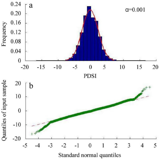
Figure 2. Normality tests for scPDSI variability across China from 1951 to 2014. The Jarque–Bera test results and the quantile–quantile plot are shown in (a,b), respectively.

In addition, special attention has been paid to extreme hydroclimatic change (|scPDSI| > 0.4) via an examination of their spatial distributions (Figure 3). As shown, the problem of the over-reporting of the extreme dry or wet conditions, which has been reported for the original PDSI dataset [2], still exists in the self-calibrated data. The over-reported extreme wet spells are not found in traditionally humid regions (e.g., South China), and instead are mainly found on the North Tibetan Plateau and in South Xinjiang (Figure 3a). Similarly, the extreme dry regimes are mainly represented in North and Southwest China instead of in traditionally semiarid and arid regions (e.g., Northwest China) (Figure 3b). In fact, the scPDSI was developed to describe the cumulative departure from the mean values in moisture supply and demand at the local surface level [31,33]. Therefore, persistent increases or decreases in moisture can give rise to the occurrence of clusters of extreme scPDSI values. This is in good agreement with many previous studies that have revealed that a persistent drying trend has been in place since the 1950s in North and Southwest China [19,40,41,42,43], while a remarkable wetting trend has been found in arid Central Asia [44].

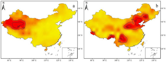
Figure 3. The frequency at which the scPDSI reported (a) an extreme wet spell (percentage of months with scPDSI < −4.0) and (b) an extreme dry spell (percentage of months with scPDSI > 4.0).

4. Spatiotemporal Evolution of Hydroclimatic Change Trends across China

The spatial evolution of the wetting or drying trends across China at a given time is presented in Figure 4. As shown, the hydroclimatic pattern in China can be termed as “eastern drying and western wetting” during the period from 1951 to 2014. The boundary of the drying land in Northern and Northeastern China (NNEC) has extended eastward, and Southwest China (SC) has also shown a drying trend in recent years. However, the Tibetan Plateau (TP) and Northwestern China (WNWC) have shown a wetting trend. In this study, only those regions with significant hydroclimatic variations are further discussed.

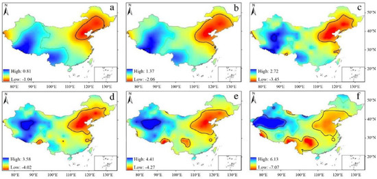
Figure 4. Spatial evolution of the EEMD-based trends of scPDSI across China ending in (a) 1960, (b) 1970, (c) 1980, (d) 1990, (e) 2000, and (f) 2014, respectively. Variations significant at the 0.05 level are highlighted by black lines. The green line symbolizes the change value of zero.

NNEC has been facing a significant and persistent downward trend in moisture availability over the past 60 years, which has caused enormous economic losses each year [45]. To alleviate the regional water-shortage problem, the South-to-North Water Diversion Project has been implemented by the central government. Previous studies have revealed that the recent decades correspond well to periods of East-Asian summer-monsoon failure which lead to deficient precipitation in NNEC [46,47]. The rapid warming in the Central and Eastern Pacific Ocean, as the primary cause for the decay of monsoon intensity, can suppress convective activity over the Philippine Sea via the descending limb of the Walker circulation [48]. The relatively cold Western Pacific Ocean and the subsidence over it weakens the Hadley circulation and thus reduces the western Pacific high, causing the failure of the summer monsoon and creating dry conditions in NNEC [22]. The recent cooling trend of the upper tropospheric temperature over East Asia was found to cause a weakening of the northward progression of regional summer-monsoon winds [49]. In addition, the radiative effects of significant increases in aerosols (e.g., black carbon) from urbanization and industrialization may stabilize the atmospheric convection, hence reducing regional monsoonal precipitation [50]. The boundary of the significantly drying land in NNEC has extended eastward to the eastern Loess Plateau and southward, close to the middle and lower reaches of the Yangtze River since 1990. This finding may be consistent with the dryland expansion experienced in northern China during the recent warming trend, as suggested by previous studies [51].

Recent decades have witnessed the most conspicuous increases in precipitation experienced on the TP over the course of the past millennium according to observations from regional tree-ring-based precipitation reconstructions [52]. However, the wetting tendency in most parts of the TP tends to be relatively moderate, except for in the northern part, which has experienced a significantly accelerated pace of wetting since 1980. One of the potential factors accounting for the wetting trends in the TP is related to large-scale oceanic and atmospheric patterns on interdecadal timescales, e.g., anomalies in the sea surface temperature (SST) of the North Indian Ocean. In recent years, the warming of the sea surface temperature in the North Indian Ocean has caused upward convection, which brings water vapor into the TP through the Walker circulation [53]. In addition, great moisture supply on the TP may be related to large-scale warming from a long-term perspective, as indicated by a significantly statistical association between moisture-sensitive tree-ring chronologies and the reconstructed Northern Hemisphere temperature [54,55,56].This warming may enhance the emissions of the biogenic volatile organic compounds from terrestrial vegetation that can increase the amount of secondary organic aerosols due to limited anthropogenic influence in the TP, contributing to the concentration of cloud condensation nuclei and leading to a regional precipitation increase [57]. It has been found that, in the past decade, the wetting regions have shrunk in the southern TP. This is mainly due to the anticyclonic trend that has appeared over the northeastern TP [58].

There were both moderate drying and weak wetting regions in the western parts of WNWC prior to 1980. Yet the drying regions shrank dramatically, and most of them turned into wetting regions over the next 3 decades. The strongest wetting rates occurred in the southern part of WNWC, especially the Tarim Basin. The moisture increase in this area was also evidenced by the observed precipitation records and other hydroclimatic data [59]. Closely associated with the regional moisture increase are two anomalous atmospheric teleconnection patterns that connect in WNWC. The zonal wave train along the middle latitudes resembles the “Silk Road Pattern”, and it induces an increase in the strength of the westerly winds, transporting moist air from the Atlantic Ocean and the Mediterranean Sea into this region [31]. The meridional pattern demonstrates a negative height anomaly in Central Asia, and positive height anomalies in tropical and subarctic areas. This wave train leads to anomalous southerly winds that bring abundant water vapor from the Arabian Sea into this area via the western boundary of the TP, and then they bend north and fuel regional precipitation development [60].

As for SC, regional moisture basically remained in a slight upward trend before 1990, and an abrupt trend reversal took place over the next 2 decades. The recent drying conditions in SC are considered to be the most dramatic over the past century [61]. The potential driving mechanisms for this dry spell seem to be quite complicated according to a large number of previous studies. The severe droughts over SC are closely linked with an anomalously strong western Pacific subtropical high (WPSH), which shifted to the north and west of its normal position. Subsidence prevailed in SC under the control of the WPSH and suppressed water-vapor transport towards this region [2]. Meanwhile, the South Asian high is stronger and lies to the east of its normal position, causing the failure of the summer southwest monsoon season [62]. The occurrence of the severe drought in SC is also related to anomalies in the westerlies’ circulation system, with anomalously high pressure over Lake Baikal and anomalously low pressure over East Asia, which can weaken the strength of southward cold air into SC and prevent the convergence of warm–moist air and cold–dry air over SC [63]. Plus, an anomalously high pressure ridge develops over the TP in very dry years, leading to the decline of the southwest monsoon and the prevalence of the dry northwesterly wind over SC [10]. In addition, the recent drying conditions in SC may be associated with the warming of the tropical oceans [64] and the Indian Ocean dipole [65].

5. Complexity of Hydroclimatic Variability in China

The spatial pattern of the HFD exponents for the scPDSI dataset over the entire domain is presented in Figure 5, which illustrates that the HFD values on a monthly scale range between 1.37 and 1.54 (Figure 5a), and the ones on an annual scale vary between 1.58 and 2.01 (Figure 5b). We found that none of HFD values is an integer, indicating that the hydroclimatic variations across the region are chaotic dynamic systems with fractal characteristics, and they are sensitive to the initial conditions [28,29,30]. A comparison of the HFD values reveals that the complexity of the hydroclimatic dynamics in China decreases along with an increase in the temporal scale. This result accords with many previous studies that demonstrated that the climate data with higher resolution often contain more details and thus are more complex [30].

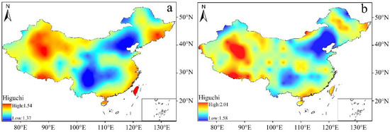
Figure 5. Spatial pattern of the HFD exponents for the scPDSI series on monthly (a) and annual (b) scales across China.

The higher HFD values are mainly distributed in WNWC and the TP, and the lower values mainly concentrate in NNEC and SC. This finding demonstrates that the hydroclimatic dynamics in WNWC and the TP are more complicated than those in NNEC and SC. This phenomenon is probably associated with the presence of atmospheric processes and landforms in different parts of the study region. Dong et al. revealed that the spatial distributions of higher fractal dimension values for temperature dynamics in the Tarim Basin were found in areas with complex landforms [66] Donner found that the spatial patterns of the HFD values for precipitation variability across the entirety of Germany were totally the opposite on the short (1–7 days) and long (10–100 days) timescales [67]. Xu et al. discovered that the complexity of temperature and precipitation dynamics in Xinjiang was positively related to elevations [28,29,30]. Previous evaluations of the circulation features of WNWC and the TP indicated that the regional moisture conditions are transported from the Indian Ocean, the Atlantic Ocean, giant lakes in Central Asia (e.g., the Caspian Sea and the Aral Sea), and the Arctic [22,29,51]. In addition, the two subareas have a unique geological feature, with an average elevation ranging from −155 m to 8848 m ASL, strongly influencing the monsoon and westerlies dynamics [68]. Therefore, the coupling of large-scale circulation and diverse geographic conditions possibly results in the poor stability and high complexity of the hydroclimatic change in WNWC and the TP.

6. Conclusions

From our study of the nonlinear characteristics of the hydroclimatic variability across China using the EEMD and the HFD method, several conclusions can be drawn, as follow:

(1) The hydroclimatic change is spatially and temporally non-uniform over the entire domain. NNEC has been facing a persistent and noticeable drying trend since the 1950s. The significant wetting conditions in the TP and WNWC started sporadically at first and strongly accelerated until around the 1980s. A slight wetting trend was found in SC before 1990, followed by the occurrence of a dramatic drying trend over the next 2 decades.

(2) None of the HFD values is an integer, which indicates that all of the hydroclimatic dynamics on the monthly and annual scales are chaotic dynamic systems with fractal characteristics, and they are sensitive to the initial conditions. The variations on a smaller temporal scale (e.g., a monthly scale) tend to be more complex than those on a larger temporal scale (e.g., an annual scale). Additionally, the hydroclimatic changes in WNWC and the TP are more complicated than those in NNEC and SC, which may be related to the complex circulation patterns and diverse geomorphic features that dominate them.

References

- Domrös, M.; Gongbing, P. Controlling Factors of the Climate. In The Climate of China; Domrös, M., Gongbing, P., Eds.; Springer: Berlin/Heidelberg, Germany, 1988; pp. 20–29. [Google Scholar]
- Li, J.; Cook, E.R.; Chen, F.; Davi, N.; D’Arrigo, R.; Gou, X.; Wright, W.E.; Fang, K.; Jin, L.; Shi, J. Summer monsoon moisture variability over China and Mongolia during the past four centuries. Geophys. Res. Lett. 2009, 36. [Google Scholar] [CrossRef]
- Yu, C.; Huang, X.; Chen, H.; Huang, G.; Ni, S.; Wright, J.S.; Hall, J.; Ciais, P.; Zhang, J.; Xiao, Y. Assessing the impacts of extreme agricultural droughts in China under climate and socioeconomic changes. Earth’s Future 2018, 6, 689–703. [Google Scholar] [CrossRef]
- Wang, M.; Ding, Z.; Wu, C.; Song, L.; Ma, M.; Yu, P.; Lu, B.; Tang, X. Divergent responses of ecosystem water-use efficiency to extreme seasonal droughts in Southwest China. Sci. Total Environ. 2021, 760, 143427. [Google Scholar] [CrossRef] [PubMed]
- Zhang, P.; Cheng, H.; Edwards, R.L.; Chen, F.; Wang, Y.; Yang, X.; Liu, J.; Tan, M.; Wang, X.; Liu, J. A test of climate, sun, and culture relationships from an 1810-year Chinese cave record. Science 2008, 322, 940–942. [Google Scholar] [CrossRef]
- Fang, K.; Gou, X.; Chen, F.; Frank, D.; Liu, C.; Li, J.; Kazmer, M. Precipitation variability during the past 400 years in the Xiaolong Mountain (central China) inferred from tree rings. Clim. Dyn. 2012, 39, 1697–1707. [Google Scholar] [CrossRef]
- Cook, E.R.; Anchukaitis, K.J.; Buckley, B.M.; D’Arrigo, R.D.; Jacoby, G.C.; Wright, W.E. Asian monsoon failure and megadrought during the last millennium. Science 2010, 328, 486–489. [Google Scholar] [CrossRef]
- Fang, K.; Gou, X.; Chen, F.; Liu, C.; Davi, N.; Li, J.; Zhao, Z.; Li, Y. Tree-ring based reconstruction of drought variability (1615–2009) in the Kongtong Mountain area, northern China. Glob. Planet. Chang. 2012, 80, 190–197. [Google Scholar] [CrossRef]
- Ding, A.J.; Xiao, S.C.; Peng, X.M.; Tian, Q.Y.; Han, C. Shrub-rings used to reconstruct drought history of the central Alxa desert, northwest China. Int. J. Climatol. 2021, 41, 4957–4965. [Google Scholar] [CrossRef]
- Zhang, W.; Jin, F.-F.; Zhao, J.-X.; Qi, L.; Ren, H.-L. The possible influence of a nonconventional El Niño on the severe autumn drought of 2009 in Southwest China. J. Clim. 2013, 26, 8392–8405. [Google Scholar] [CrossRef]
- Yan, G.; Wu, Z.; Li, D. Comprehensive analysis of the persistent drought events in Southwest China. Disaster Adv. 2013, 6, 306–315. [Google Scholar]
- Peng, X.; Yang, B.; Xiao, S.; Liu, J.; Li, G. Hydroclimate Correlations Between the Alxa Desert and Adjacent Mountains in Northwestern China: Evidence from Meteorological and Tree-Ring Data. J. Geophys. Res. Atmos. 2021, 126, e2021JD035006. [Google Scholar] [CrossRef]
- Pan, Y.; Li, Q.; Liu, Y.; Liu, R.; Deng, R. Hydroclimate variations in the Northern China Plain and their possible socio-cultural influences. Geogr. Ann. Ser. A Phys. Geogr. 2020, 102, 287–296. [Google Scholar] [CrossRef]
- Zhang, E.; Zhao, C.; Xue, B.; Liu, Z.; Yu, Z.; Chen, R.; Shen, J. Millennial-scale hydroclimate variations in southwest China linked to tropical Indian Ocean since the Last Glacial Maximum. Geology 2017, 45, 435–438. [Google Scholar] [CrossRef]
- Zhou, F.; Fang, K.; Zhang, F.; Dong, Z. Hydroclimate change encoded in tree rings of Fengshui woods in Southeastern China and its teleconnection with El Niño-Southern Oscillation. Water Resour. Res. 2020, 56, e2018WR024612. [Google Scholar] [CrossRef]
- Ljungqvist, F.C.; Krusic, P.J.; Sundqvist, H.S.; Zorita, E.; Brattström, G.; Frank, D. Northern Hemisphere hydroclimate variability over the past twelve centuries. Nature 2016, 532, 94–98. [Google Scholar] [CrossRef]
- Sang, Y.-F.; Sun, F.; Singh, V.P.; Xie, P.; Sun, J. A discrete wavelet spectrum approach for identifying non-monotonic trends in hydroclimate data. Hydrol. Earth Syst. Sci. 2018, 22, 757–766. [Google Scholar] [CrossRef]
- Qian, Y.; Leung, L.R. A long-term regional simulation and observations of the hydroclimate in China. J. Geophys. Res. Atmos. 2007, 112. [Google Scholar] [CrossRef]
- Zou, X.; Zhai, P.; Zhang, Q. Variations in droughts over China: 1951–2003. Geophys. Res. Lett. 2005, 32. [Google Scholar] [CrossRef]
- Bai, L.; Xu, J.; Chen, Z.; Li, W.; Liu, Z.; Zhao, B.; Wang, Z. The regional features of temperature variation trends over Xinjiang in China by the ensemble empirical mode decomposition method. Int. J. Climatol. 2015, 35, 3229–3237. [Google Scholar] [CrossRef]
- Ji, F.; Wu, Z.; Huang, J.; Chassignet, E.P. Evolution of land surface air temperature trend. Nat. Clim. Chang. 2014, 4, 462–466. [Google Scholar] [CrossRef]
- Zhou, F.; Fang, K.; Li, Y.; Chen, Q.; Chen, D. Nonlinear characteristics of hydroclimate variability in the mid-latitude Asia over the past seven centuries. Theor. Appl. Climatol. 2016, 126, 151–159. [Google Scholar] [CrossRef]
- Wu, Z.; Huang, N.E. Ensemble empirical mode decomposition: A noise-assisted data analysis method. Adv. Adapt. Data Anal. 2009, 1, 1–41. [Google Scholar] [CrossRef]
- Lorenzelli, F. The Essence of Chaos; CRC Press: Boca Raton, FL, USA, 2014. [Google Scholar]
- Pierce, D.W.; Barnett, T.P.; Santer, B.D.; Gleckler, P.J. Selecting global climate models for regional climate change studies. Proc. Natl. Acad. Sci. USA 2009, 106, 8441–8446. [Google Scholar] [CrossRef]
- Millán, H.; Kalauzi, A.; Llerena, G.; Sucoshañay, J.; Piedra, D. Meteorological complexity in the Amazonian area of Ecuador: An approach based on dynamical system theory. Ecol. Complex. 2009, 6, 278–285. [Google Scholar] [CrossRef]
- Liu, Z.; Xu, J.; Shi, K. Self-organized criticality of climate change. Theor. Appl. Climatol. 2014, 115, 685–691. [Google Scholar] [CrossRef]
- Xu, J.; Chen, Y.; Li, W.; Dong, S. Long-term trend and fractal of annual runoff process in mainstream of Tarim River. Chin. Geogr. Sci. 2008, 18, 77–84. [Google Scholar] [CrossRef]
- Xu, J.; Chen, Y.; Li, W.; Liu, Z.; Wei, C.; Tang, J. Understanding the complexity of temperature dynamics in Xinjiang, China, from multitemporal scale and spatial perspectives. Sci. World J. 2013, 2013, 259248. [Google Scholar]
- Xu, J.; Chen, Y.; Li, W.; Liu, Z.; Tang, J.; Wei, C. Understanding temporal and spatial complexity of precipitation distribution in Xinjiang, China. Theor. Appl. Climatol. 2016, 123, 321–333. [Google Scholar] [CrossRef]
- Dai, A. Characteristics and trends in various forms of the Palmer Drought Severity Index during 1900–2008. J. Geophys. Res. Atmos. 2011, 116. [Google Scholar] [CrossRef]
- Palmer, W.C. Meteorological Drought; US Department of Commerce, Weather Bureau: Washington, DC, USA, 1965; Volume 30.
- Dai, A.; Trenberth, K.E.; Qian, T. A global dataset of Palmer Drought Severity Index for 1870–2002: Relationship with soil moisture and effects of surface warming. J. Hydrometeorol. 2004, 5, 1117–1130. [Google Scholar] [CrossRef]
- Huang, N.E.; Shen, Z.; Long, S.R.; Wu, M.C.; Shih, H.H.; Zheng, Q.; Yen, N.-C.; Tung, C.C.; Liu, H.H. The empirical mode decomposition and the Hilbert spectrum for nonlinear and non-stationary time series analysis. Proc. R. Soc. Lond. Ser. A Math. Phys. Eng. Sci. 1998, 454, 903–995. [Google Scholar] [CrossRef]
- Higuchi, T. Approach to an irregular time series on the basis of the fractal theory. Phys. D Nonlinear Phenom. 1988, 31, 277–283. [Google Scholar] [CrossRef]
- Kesić, S.; Spasić, S.Z. Application of Higuchi’s fractal dimension from basic to clinical neurophysiology: A review. Comput. Methods Programs Biomed. 2016, 133, 55–70. [Google Scholar] [CrossRef]
- Gómez, C.; Mediavilla, Á.; Hornero, R.; Abásolo, D.; Fernández, A. Use of the Higuchi’s fractal dimension for the analysis of MEG recordings from Alzheimer’s disease patients. Med. Eng. Phys. 2009, 31, 306–313. [Google Scholar] [CrossRef]
- Ahmadi, B.; Amirfattahi, R. Comparison of correlation dimension and fractal dimension in estimating BIS index. Wirel. Sens. Netw. 2010, 2, 67. [Google Scholar] [CrossRef][Green Version]
- Coyt, G.G.; Diosdado, A.M.; López, J.A.B.; del Rio Correa, J.L.; Brown, F.A. Higuchi’s Method applied to the detection of periodic components in time series and its application to seismograms. Rev. Mex. Física 2013, 59, 1–6. [Google Scholar]
- Huang, J.; Yu, H.; Guan, X.; Wang, G.; Guo, R. Accelerated dryland expansion under climate change. Nat. Clim. Chang. 2016, 6, 166–171. [Google Scholar] [CrossRef]
- Zhao, X.; Zhang, F.; Su, R.; Gao, C.; Xing, K. Response of carbon and water fluxes to dryness/wetness in China. Terr. Atmos. Ocean. Sci. 2021, 32, 53–67. [Google Scholar] [CrossRef]
- Li, Z.; Yang, S.; He, B.; Hu, C. Intensified springtime deep convection over the South China Sea and the Philippine Sea dries southern China. Sci. Rep. 2016, 6, 30470. [Google Scholar] [CrossRef]
- Xu, H.-j.; Wang, X.-p.; Zhao, C.-y.; Shan, S.-y.; Guo, J. Seasonal and aridity influences on the relationships between drought indices and hydrological variables over China. Weather Clim. Extrem. 2021, 34, 100393. [Google Scholar] [CrossRef]
- Ta, Z.; Yu, R.; Chen, X.; Mu, G.; Guo, Y. Analysis of the spatio-temporal patterns of dry and wet conditions in Central Asia. Atmosphere 2018, 9, 7. [Google Scholar] [CrossRef]
- Zhang, X.; Liu, X.; Wang, W.; Zhang, T.; Zeng, X.; Xu, G.; Wu, G.; Kang, H. Spatiotemporal variability of drought in the northern part of northeast China. Hydrol. Process. 2018, 32, 1449–1460. [Google Scholar] [CrossRef]
- Liu, L.; Zhang, R.; Zuo, Z. Effect of spring precipitation on summer precipitation in eastern China: Role of soil moisture. J. Clim. 2017, 30, 9183–9194. [Google Scholar] [CrossRef]
- Chang, X.; Wang, B.; Yan, Y.; Hao, Y.; Zhang, M. Characterizing effects of monsoons and climate teleconnections on precipitation in China using wavelet coherence and global coherence. Clim. Dyn. 2019, 52, 5213–5228. [Google Scholar] [CrossRef]
- Kumar, K.K.; Rajagopalan, B.; Cane, M.A. On the weakening relationship between the Indian monsoon and ENSO. Science 1999, 284, 2156–2159. [Google Scholar] [CrossRef]
- Yu, R.; Wang, B.; Zhou, T. Tropospheric cooling and summer monsoon weakening trend over East Asia. Geophys. Res. Lett. 2004, 31. [Google Scholar] [CrossRef]
- Meehl, G.A.; Arblaster, J.M.; Collins, W.D. Effects of black carbon aerosols on the Indian monsoon. J. Clim. 2008, 21, 2869–2882. [Google Scholar] [CrossRef]
- Huang, W.; Feng, S.; Chen, J.; Chen, F. Physical mechanisms of summer precipitation variations in the Tarim Basin in northwestern China. J. Clim. 2015, 28, 3579–3591. [Google Scholar] [CrossRef]
- Shao, X.; Xu, Y.; Yin, Z.Y.; Liang, E.; Zhu, H.; Wang, S. Climatic implications of a 3585-year tree-ring width chronology from the northeastern Qinghai-Tibetan Plateau. Quat. Sci. Rev. 2010, 29, 2111–2122. [Google Scholar] [CrossRef]
- Zhao, Y.; Duan, A.; Wu, G. Interannual variability of late-spring circulation and diabatic heating over the Tibetan Plateau associated with Indian Ocean forcing. Adv. Atmos. Sci. 2018, 35, 927–941. [Google Scholar] [CrossRef]
- Wang, J.; Yang, B.; Ljungqvist, F.C. Moisture and temperature covariability over the Southeastern Tibetan Plateau during the Past Nine Centuries. J. Clim. 2020, 33, 6583–6598. [Google Scholar] [CrossRef]
- Li, J.; Shi, J.; Zhang, D.D.; Yang, B.; Fang, K.; Yue, P.H. Moisture increase in response to high-altitude warming evidenced by tree-rings on the southeastern Tibetan Plateau. Clim. Dyn. 2017, 48, 649–660. [Google Scholar] [CrossRef]
- Qin, C.; Yang, B.; Burchardt, I.; Hu, X.; Kang, X. Intensified pluvial conditions during the twentieth century in the inland Heihe River Basin in arid northwestern China over the past millennium. Glob. Planet. Chang. 2010, 72, 192–200. [Google Scholar] [CrossRef]
- Paasonen, P.; Asmi, A.; Petäjä, T.; Kajos, M.K.; Äijälä, M.; Junninen, H.; Holst, T.; Abbatt, J.P.D.; Arneth, A.; Birmili, W. Warming-induced increase in aerosol number concentration likely to moderate climate change. Nat. Geosci. 2013, 6, 438–442. [Google Scholar] [CrossRef]
- Wang, Z.; Yang, S.; Luo, H.; Li, J. Drying tendency over the southern slope of the Tibetan Plateau in recent decades: Role of a CGT-like atmospheric change. Clim. Dyn. 2022, 1–13. [Google Scholar] [CrossRef]
- Li, J.; Gou, X.; Cook, E.R.; Chen, F. Tree-ring based drought reconstruction for the central Tien Shan area in northwest China. Geophys. Res. Lett. 2006, 33. [Google Scholar] [CrossRef]
- Fang, K.; Gou, X.; Chen, F.; Li, J.; D’Arrigo, R.; Cook, E.; Yang, T.; Davi, N. Reconstructed droughts for the southeastern Tibetan Plateau over the past 568 years and its linkages to the Pacific and Atlantic Ocean climate variability. Clim. Dyn. 2010, 35, 577–585. [Google Scholar] [CrossRef]
- Lin, W.; Wen, C.; Wen, Z.; Gang, H. Drought in Southwest China: A review. Atmos. Ocean. Sci. Lett. 2015, 8, 339–344. [Google Scholar]
- Yang, J.; Liu, Q.; Xie, S.P.; Liu, Z.; Wu, L. Impact of the Indian Ocean SST basin mode on the Asian summer monsoon. Geophys. Res. Lett. 2007, 34. [Google Scholar] [CrossRef]
- Zhang, C. Moisture sources for precipitation in Southwest China in summer and the changes during the extreme droughts of 2006 and 2011. J. Hydrol. 2020, 591, 125333. [Google Scholar] [CrossRef]
- Tan, L.; Cai, Y.; An, Z.; Cheng, H.; Shen, C.-C.; Gao, Y.; Edwards, R.L. Decreasing monsoon precipitation in southwest China during the last 240 years associated with the warming of tropical ocean. Clim. Dyn. 2017, 48, 1769–1778. [Google Scholar] [CrossRef]
- Xu, C.; An, W.; Wang, S.Y.S.; Yi, L.; Ge, J.; Nakatsuka, T.; Sano, M.; Guo, Z. Increased drought events in southwest China revealed by tree ring oxygen isotopes and potential role of Indian Ocean Dipole. Sci. Total Environ. 2019, 661, 645–653. [Google Scholar] [CrossRef]
- Dong, S.; Xu, J.; Chen, Y.; Li, W. Fractal characteristics of annual mean temperature of the Tarim Basin. Arid Land Geogr. 2009, 32, 17–22. [Google Scholar]
- Donner, R.V. Complexity concepts and non-integer dimensions in climate and paleoclimate research. In Fractal Analysis and Chaos in Geosciences; Intech: London, UK, 2012; pp. 1–28. [Google Scholar]
- Bansod, S.D.; Yin, Z.Y.; Lin, Z.; Zhang, X. Thermal field over Tibetan Plateau and Indian summer monsoon rainfall. Int. J. Climatol. J. R. Meteorol. Soc. 2003, 23, 1589–1605. [Google Scholar] [CrossRef]
Publisher’s Note: MDPI stays neutral with regard to jurisdictional claims in published maps and institutional affiliations. |
© 2022 by the authors. Licensee MDPI, Basel, Switzerland. This article is an open access article distributed under the terms and conditions of the Creative Commons Attribution (CC BY) license (https://creativecommons.org/licenses/by/4.0/).