Suppressing Grid-Point Storms in a Numerical Forecasting Model

Abstract

The convective parameterization scheme of the Korean Integrated Model (KIM) is tentatively modified to suppress grid-point storms in the Western Pacific Ocean. The KIM v3.2.11 suffers from the numerical problem that grid-point storms degrade forecasts in the tropical oceans and around the Korean Peninsula. Another convective parameterization scheme, the new Tiedtke scheme, is implemented in the KIM. The artificial storms are suppressed in the test version because the heating and drying tendencies of the new Tiedtke scheme are stronger than those of the default KIM Simplified Arakawa-Schubert (KSAS) scheme. Based on this comparison, the KSAS scheme is modified to strengthen its heating and drying tendencies by reducing the entrainment and detrainment rates. The modified KSAS scheme suppresses grid-point storms and thus decreases grid-scale precipitation in a summertime case simulation. Twenty 10-day forecasts with the default convection scheme (KSAS) and twenty forecasts with the modified scheme are conducted and compared with each other, confirming that the modified KSAS scheme successfully suppresses grid-point storms.

1. Introduction

Improving precipitation processes in numerical weather prediction and climate models is one of the most important but difficult tasks for achieving better weather and climate prediction [1,2]. Numerical models generally simulate clouds and precipitation using two kinds of parameterization schemes—cloud microphysics and deep/shallow cumulus convection schemes—which handle grid-scale and subgrid-scale moist processes, respectively. By generating clouds (precipitating), the two schemes remove grid-scale supersaturation and convective instability, respectively, stabilizing cloudy space. However, unrealistic weather events can occur intermittently or systematically unless moist instabilities are sufficiently eliminated. One example is the grid-point storm, which develops from weak moist disturbances through positive feedback from grid-scale condensation, latent heat release, and surface pressure drop and convergence. Grid-point storms are often embedded in convectively unstable events (e.g., a squall line or a mesoscale convective complex), lasting several hours and severely degrading numerical forecasts [3,4]. One simple way to suppress them is to make cumulus convection stronger to deplete more convective instability, as Han and Pan [2] suppressed unrealistic grid-point storms in Southern Alabama. However, overactive subgrid convection can also suppress real convective events themselves and cause biases of precipitation and other variables. Thus, the two cloud parameterization schemes should be well-balanced to predict precipitation accurately but also remove instabilities sufficiently.

The Korean Integrated Model (KIM [5]) v3.2.11, updated in December 2018, also suffers from grid-point storms in the Western Pacific Ocean. Unrealistic excessive grid-scale precipitation tends to appear around tropical disturbances or cyclones in the Philippine Sea and the East China Sea in the late forecast period (e.g., after 7 days in the 10-day forecast). The grid-point storms often survive several days and impact nearby northward tropical cyclones (TCs), affecting convergent flow ahead of the TCs and precipitation over the Korean Peninsula. This kind of pattern deteriorates the boreal summertime skill scores of the KIM severely, thus we have been trying to mitigate this problem.

In this study, a different convection scheme is first implemented in the KIM and tested to show the sensitivity of the grid-point storms to the convection schemes. Then, the deep convection scheme in the KIM is modified to suppress the grid-point storms in the Western Pacific Ocean. The selected boreal summertime case and numerical experiments are described in Section 2, and the results are presented in Section 3. A summary and conclusions are given in Section 4.

2. Numerical Experiments

2.1. KIM and a Case Description

The KIM, a newly developed non-hydrostatic global weather forecasting model, employs the spectral element method in horizontal discretization and the finite difference method in vertical discretization over a NE360 ($\Delta \sim 12.5$ km) cubed sphere grid [6,7], with observation data processing and data assimilation over its native grid [8,9]. The physics package modules that are used in this study include radiation [10], cloudiness [11], land surface processes [12,13], ocean surface processes [14,15], vertical diffusion [16,17], subgrid orographic drag [18], and non-orographic gravity wave drag [19]. Grid-scale condensation and precipitation in the KIM are parameterized by the Weather Research and Forecasting (WRF) single-moment 5-class (WSM5) microphysics scheme [20,21]. Recently, the WSM5 scheme in the KIM was revised to consider partial cloudiness in which microphysical properties in clear and in-cloud parts are calculated separately [22]. The other type of precipitation, convective precipitation, is parameterized by shallow or deep convection schemes depending on the depth of the cumulus. The Global Forecast System (GFS) shallow convection scheme [2] is used to calculate the convective precipitation amount from cumulus shallower than 150 hPa. The convective precipitation from deeper cumulus is calculated by a modified version of the Simplified Arakawa-Schubert convection scheme in the KIM (KSAS), in which several modifications to the subgrid-scale properties were made [23,24,25,26].

In the KIM v3.2.11, grid-point storms frequently appear around tropical disturbances or TCs in the boreal summertime in the Western Pacific Ocean. They degrade forecasts in the tropics and around the Korean Peninsula by affecting the tracks and intensities of northward-moving TCs. To investigate their sensitivity to convective parameterization schemes, we select one boreal summertime period (19–29 July 2017) when tropical disturbances were active in the Western Pacific Ocean and some of them developed into TCs (e.g., TCs Noru, Kulap, and Nesat; Figure 1a–e). A 10-day control experiment with the current KIM physics package (CTL hereafter) is conducted starting at 0000 UTC on 19 July 2017. The European Centre for Medium-Range Weather Forecasts (ECMWF) fifth major global reanalysis data, ERA5 [27] are remapped on the cubed-sphere grid with NE360 horizontal resolution and 91 vertical levels, and the remapped data are used as the initial conditions of the CTL experiment. The simulation results are saved every six hours for analysis.

The CTL simulation results, interpolated to the 0.125°×0.125° latitude–longitude grid, are compared with the 0.25°×0.25° precipitation measurements in the tropical and subtropical regions from the Tropical Rainfall Measuring Mission (TRMM) Multi-Satellite Precipitation Analysis (TMPA) observations (Figure 1). Details of TMPA observations can be found in [28]. In the CTL experiment, there were tropical disturbances or TC-like vortices in the Western Pacific Ocean during the initial period (Figure 1f) and they evolved to two strong TCs during the final period (Figure 1j). During the transition stage, one strong grid-point storm developed on the east side of the TC in the Philippine Sea (Figure 1h) and it affected the TC afterwards (Figure 1i,j). Tropical disturbances and grid-point storms become more active after 0000 UTC on 24 July 2017 (five-day integration). Therefore, we perform two restart runs from the initial five-day CTL integration with different convective parameterization schemes to investigate the sensitivity of the convective activity to the convective instability and its parameterization (see Section 2.2).

2.2. New Tiedtke Scheme (NTDK) and MOD Experiments

We first examine the grid-point storms in our test version with the convective parameterization schemes replaced with the new Tiedtke scheme. The new Tiedtke scheme uses the mass-flux approach to represent deep, shallow, and mid-level subgrid convections, as did its original version [29]. In this newly modified scheme, a moisture convergence closure is replaced with a convective available potential energy closure to improve diurnal cycles [30], and the entrainment formulation is modified to better represent tropical variability [1]. The new Tiedtke scheme also improves the simulation of marine boundary layer clouds over the Southeast Pacific Ocean [31]. In this study, a five-day experiment with the new Tiedtke scheme (NTDK hereafter) is performed starting with the five-day integrated CTL data at 0000 UTC on 24 July 2017. The CTL and NTDK experiments are compared in Section 3.1.

Based on the comparison of the CTL and NTDK experiments (Section 3.1), the default deep convection scheme in the KIM (KSAS) is tentatively modified. The entrainment and detrainment rates in the default KSAS scheme are defined according to [1]:

$$ϵ={ϵ}_0{\left(\frac{q_s}{q_{sb}}\right)}^2+d_1(1-\mathrm{RH}){\left(\frac{q_s}{q_{sb}}\right)}^3,$$

(1)

$$\delta ={ϵ}_0,$$

(2)

$${ϵ}_0=\frac{c_1}{z_b},$$

(3)

where ${ϵ}_0$ is the entrainment rate at the cloud base, $z_b$ is the cloud base height, $c_1$ is 0.1 in the default scheme, $q_s$ is the saturation mixing ratio, $q_{sb}$ is the saturation mixing ratio at the cloud base, RH is relative humidity, and $d_1$ is 10${}^{-3}$ m${}^{-1}$. The constant $c_1$ is reduced to 0.07, and a five-day experiment with the modified KSAS scheme (MOD hereafter) is conducted, starting with the five-day integrated CTL data at 0000 UTC on 24 July 2017. Along with the MOD experiment, $c_1$ values of 0.05, 0.06, 0.08, and 0.09 are tested, and the MOD experiment produces the most satisfactory results (not shown). The impacts of the reduced entrainment and detrainment rates on grid-point storms are discussed in Section 3.

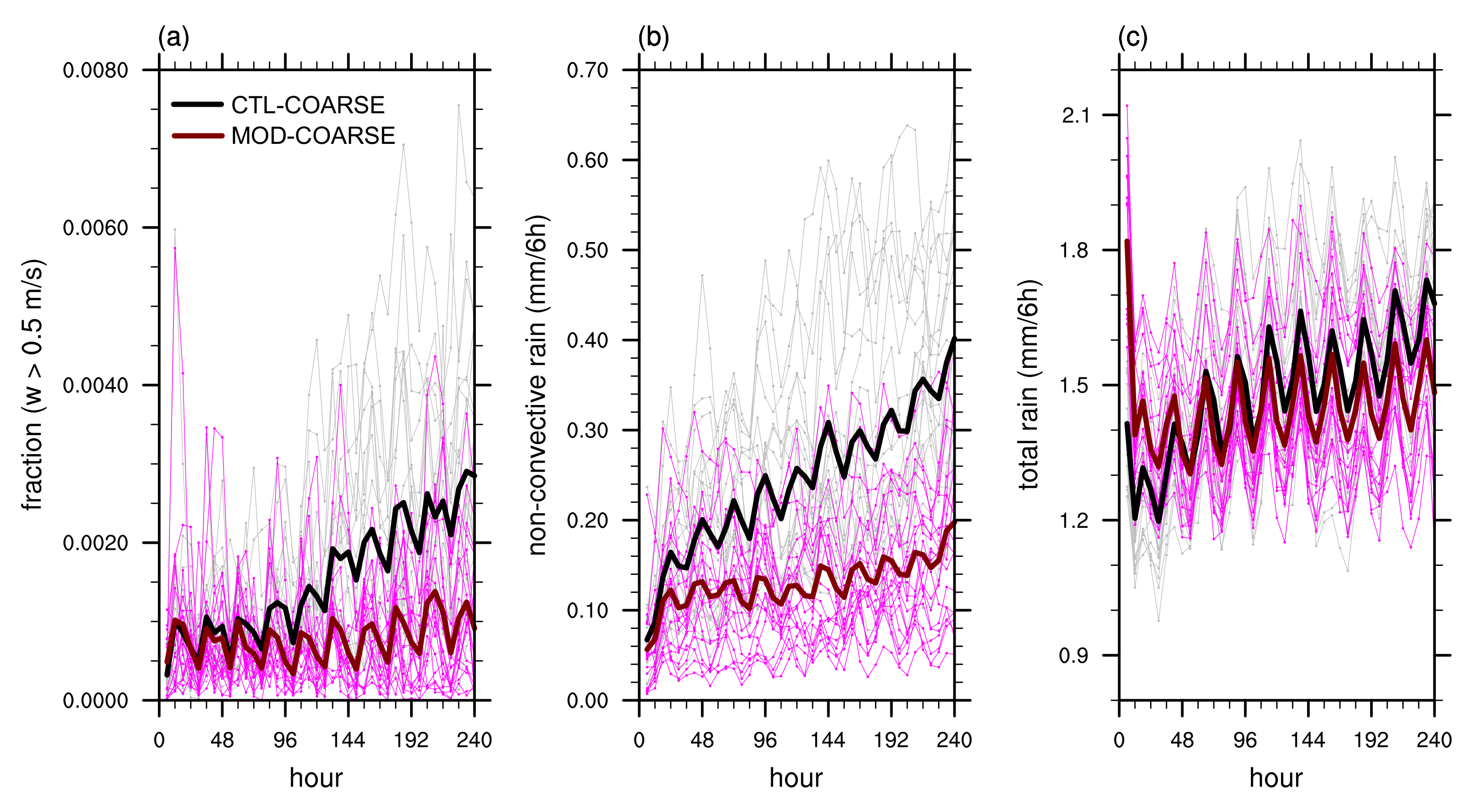
2.3. CTL-COARSE, NTDK-COARSE, and MOD-COARSE Experiments

Although the impacts of entrainment and detrainment rates reduction are distinct in the CTL and MOD case simulations, more cases are required to clarify the impacts. Thus, three sets of forecasts are performed and compared with each other. Due to our limited computing resources, coarser horizontal resolution NE180 grid (∼25 km grid interval) is used in these experiments, but the original vertical resolution is used. Twenty 10-day forecasts with the default physics package (CTL-COARSE hereafter) starting at 0000 UTC on 1–20 July 2017, respectively, are performed, and the same suite of experiments but with the modified KSAS scheme (MOD-COARSE hereafter) is conducted simultaneously. For the comparison of overall performance, a suite of experiments with the new Tiedtke scheme (NTDK-COARSE hereafter) is conducted together. The ERA5 data are remapped on the NE180 grid with 91 vertical levels for each day in the period of 1–20 July 2017 and the remapped data are used as the initial conditions of the three suites of experiments. The results are presented at the end of Section 3.

3. Results and Discussion

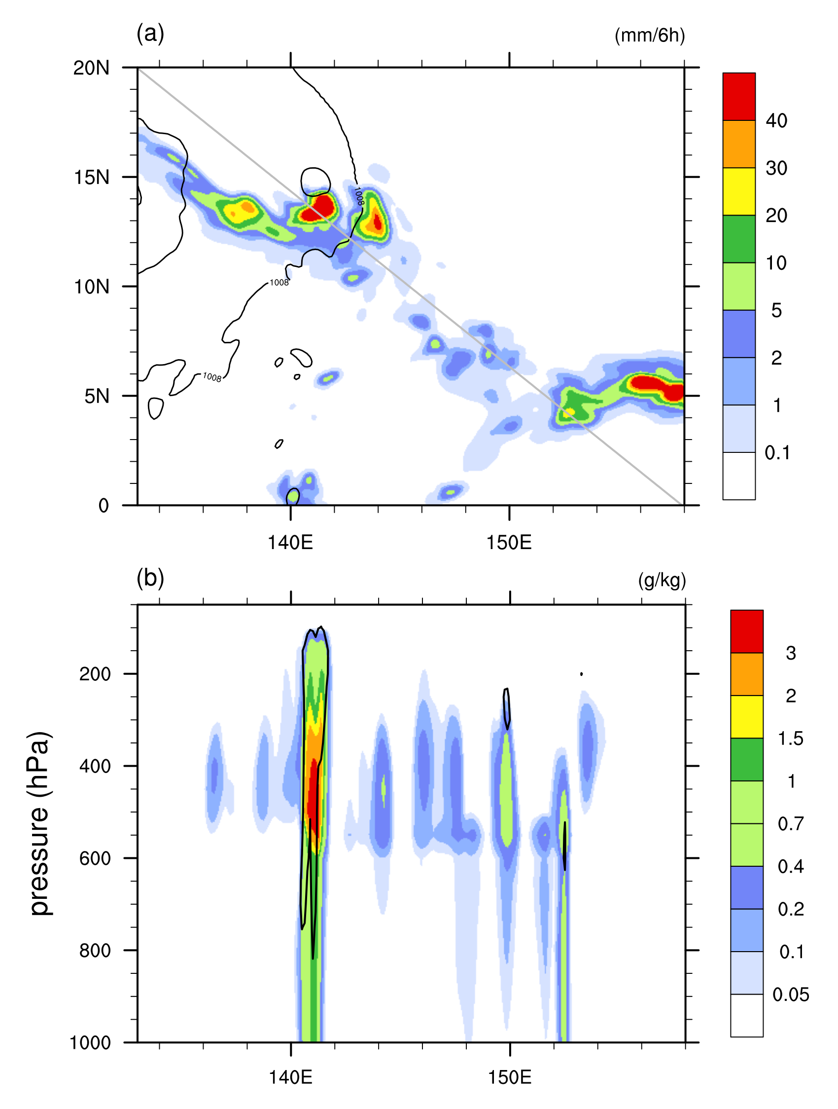
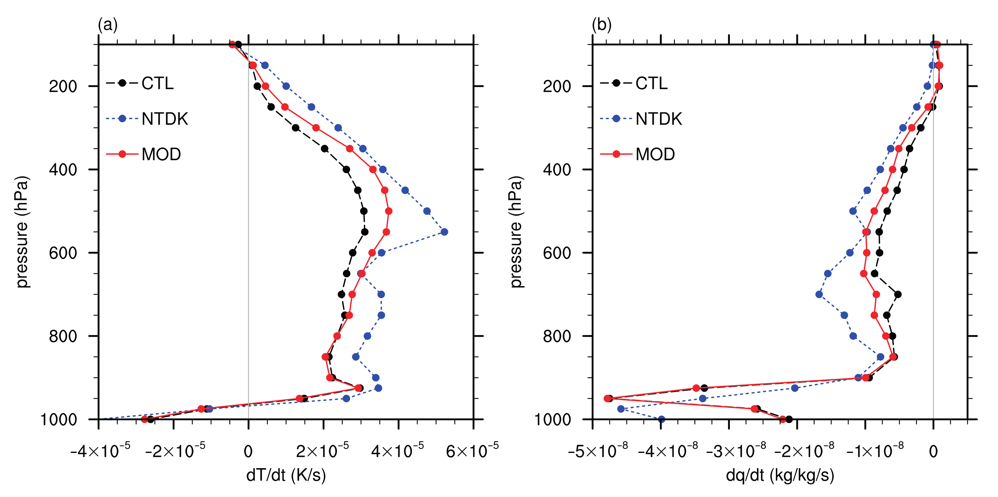
3.1. Grid-Point Storms and Heating and Drying Tendencies

As seen in Figure 1h, one strong grid-point storm emerges on the east side of the TC in the Philippine Sea, and it affects the TC afterwards in the CTL experiment (Figure 1i,j). The TC in the Philippine Sea in the CTL experiment seems to be the TC Nesat, which develops a few days earlier than observation. Figure 2 shows the grid-point storm and weaker (light green) grid-scale precipitation cores at forecast hour 132 (12 h after the five-day integration) in the CTL experiment. The grid-point storm appears as a strong updraft filled with snow and rain, extending upward to ∼100 hPa (Figure 2b). Several weaker updrafts (vertical velocity less than 0.4 m s${}^{-1}$) appear in the cross section across the gray line in Figure 2a, but rain from the updrafts evaporates below ∼600 hPa without touching the bottom. This indicates that there are many grid-point storm candidates in the area of interest.

To investigate the activity of (potential) grid-point storms, we calculate the fraction of excessively strong updrafts and the fraction of heavy grid-scale precipitation. The fraction of grid columns where the maximum vertical velocity is greater than 1 m s${}^{-1}$ and the fraction of grid columns where the six-hour accumulated grid-scale precipitation amount is greater than 80 mm in the selected domain (100° E–160° W, 0–50° N) are presented in Figure 3. In the CTL experiment, both fractions tend to increase with time, implying the continuous development of grid-point storms. In contrast, the fractions in the other two five-day restart experiments do not increase with time. The grid-point storms and weak updrafts observed after the five-day integration in the CTL experiment seem to be suppressed in the NTDK and MOD restart experiments.

The stabilizing impact of the new Tiedtke scheme is examined by analyzing the heating and drying tendencies of the convection schemes. The vertical profiles of the heating and drying tendencies averaged over the selected domain in the CTL, NTDK, and MOD experiments are shown in Figure 4. The heating and drying (negative moistening) tendencies in the NTDK experiment are stronger than those in the CTL experiment, illustrating that the parameterized subgrid overturning circulations and subgrid subsidence heating and drying in the new Tiedtke scheme are stronger than those in the default KSAS scheme. To check the significance of the differences between the CTL and NTDK experiments, we perform t-tests for the heating and drying tendencies between 900- and 200-hPa levels, and the p-values are almost zero (<10${}^{-6}$), indicating statistically significant differences. The suppression of grid-point storms in the NTDK experiment (Figure 3) is attributable to the stronger heating and drying tendencies in the NTDK experiment than in the CTL experiment, and thus the MOD experiment is designed to have stronger heating and drying tendencies to better stabilize the tropical atmosphere. For the CTL and MOD experiments, the p-values of the heating and drying tendencies between 900- and 200-hPa levels are 0.027 and 0.024, respectively, showing statistically significantly enhanced heating and drying tendencies at the 95% confidence level in the MOD experiment as we designed.

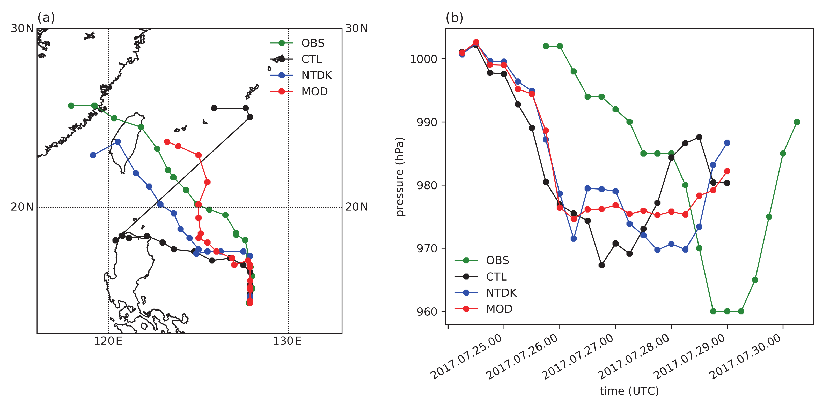
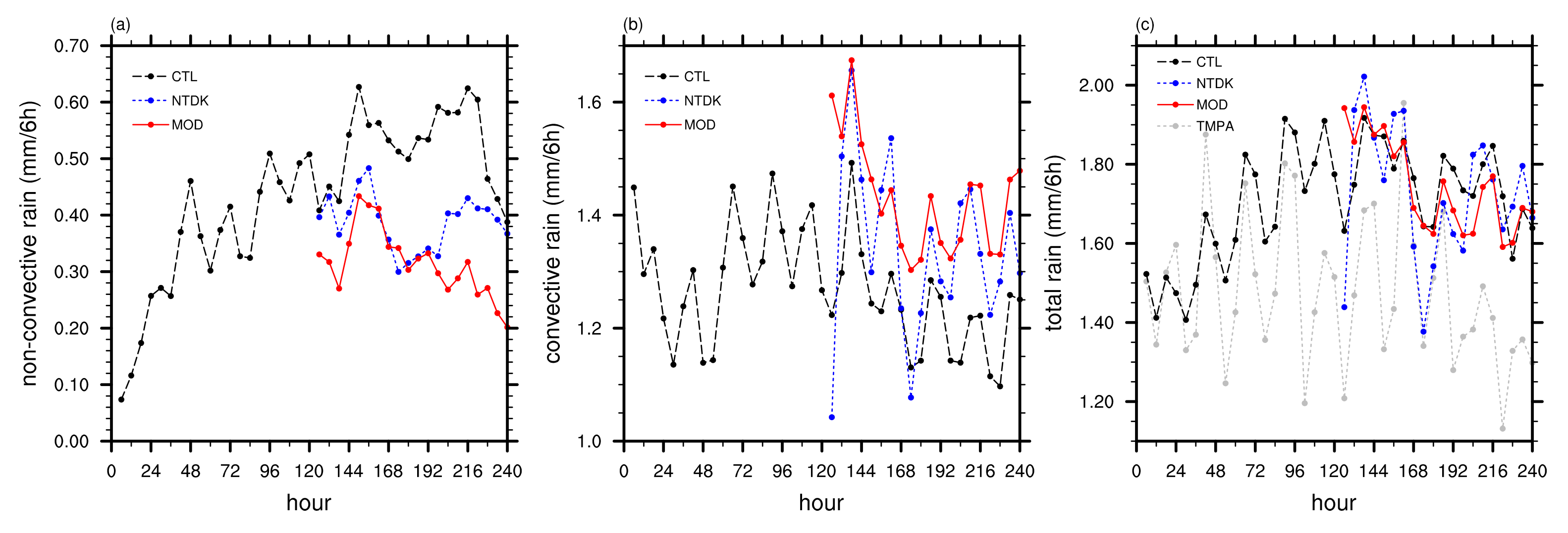
3.2. Impact of Convection Scheme Modification: Case Experiment

The magnitude of the tendencies in the MOD experiment, in which the entrainment and detrainment rates are reduced, falls between the magnitudes of the CTL and NTDK experiments (Figure 4). Due to the greater heating and drying in the MOD experiment than in the CTL experiment, a 12-h integration with the stronger deep convection scheme alone can suppress the grid-point storm and updrafts, as shown in Figure 5. When compared with the CTL experiment (Figure 2), the intensities of the updrafts and grid-scale precipitation in the MOD experiment are considerably lower, and many of the grid-scale precipitation cores disappear.

The grid-scale precipitation rates in the CTL, NTDK, and MOD experiments are shown in Figure 6. The grid-point storm on the east side of the TC Nesat strengthens at forecast hour 144, and the pre-existing TC merges with the strengthened grid-point storm after forecast hour 192 in the CTL experiment (Figure 6c). In contrast, the signature of the grid-point storm disappears at forecast hour 240 in the NTDK experiment, and the TC moves northward to the southeast coastal region of China. While the tropical disturbances completely disappear in the Western Pacific Ocean in the NTDK experiment, the tropical disturbances—or the signature of the grid-point storm—survive until the end of the MOD experiment (Figure 6i). However, their magnitude is weaker than in the CTL experiment, and the pre-existing TC moves northward to the southeast coastal region of China as in the NTDK experiment (Figure 6f,i).

To understand more on the impacts of the grid point storm, the trajectories and intensities (minimum sea-level pressure) of the TC Nesat are calculated using a simple TC tracking method (Figure 7). Using the TC information from the Korea Meteorological Administration (KMA), the latitudinal and longitudinal ranges of a target TC are calculated first, and then the locations of the minimum sea-level pressure in the area are detected in each experiment. In all the experiments, the minimum sea-level pressure starts to fall a few days earlier than observation, indicating the earlier development of the TC in the KIM simulations (Figure 7b). It is also notable that the simulated minimum sea-level pressure is higher than observation. Despite the preceding TC development, the simulated TCs follow the observed trajectory of the TC Nesat except the TC in the CTL experiment. In the CTL experiment, the TC moves westward to the Philippine until 0600 UTC on 28 July 2017, and then its center moves northeastward due to the merger of the TC with the stronger grid point storm. In the NTDK and MOD experiments, on the other hand, the grid point storm is suppressed and the TC Nesat moves northwestward, consistent with the observed trajectory (Figure 7a). Thus, the suppression of grid point storms can improve the track forecasts of TCs, especially in the late period of mid-range forecasts.

Figure 8 shows the time series of area-averaged six-hourly grid-scale, subgrid-scale convective, and total precipitation rates. When compared with the CTL experiment, the grid-scale precipitation rate decreases and the convective precipitation rate increases in the NTDK experiment (Figure 8a,b). The p-values for the area-averaged grid-scale and subgrid-scale precipitation rates are less than 0.01, showing the significance of the differences between the CTL and NTDK experiments. As in the NTDK experiment, the modified convection scheme yields more convective precipitation than in the CTL experiment due to enhanced subgrid convection (Figure 8b), and the grid-scale precipitation from the microphysics scheme decreases due to the less artificial condensation in the MOD experiment (Figure 8a). This trend is confirmed by the p-values for the area-averaged grid-scale and subgrid-scale precipitation rates in the CTL and MOD experiments, which are $9.2\times {10}^{-12}$ and $1.1\times {10}^{-7}$, respectively. Because of the increased convective precipitation rates in the NTDK and MOD experiments, the total precipitation, which is the sum of the two types of precipitation, is similar in magnitude in all three experiments, except that the rate in the NTDK experiment shows more variability over time. The p-value of the total precipitation rate for the CTL and NTDK experiments is 0.56, and the one for the CTL and MOD experiments is 0.83, indicating that the differences in the total precipitation rate are not statistically significant. It is also notable that the total precipitation rates in the late forecast period in all three experiments are larger than the TMPA precipitation rate (Figure 8c).

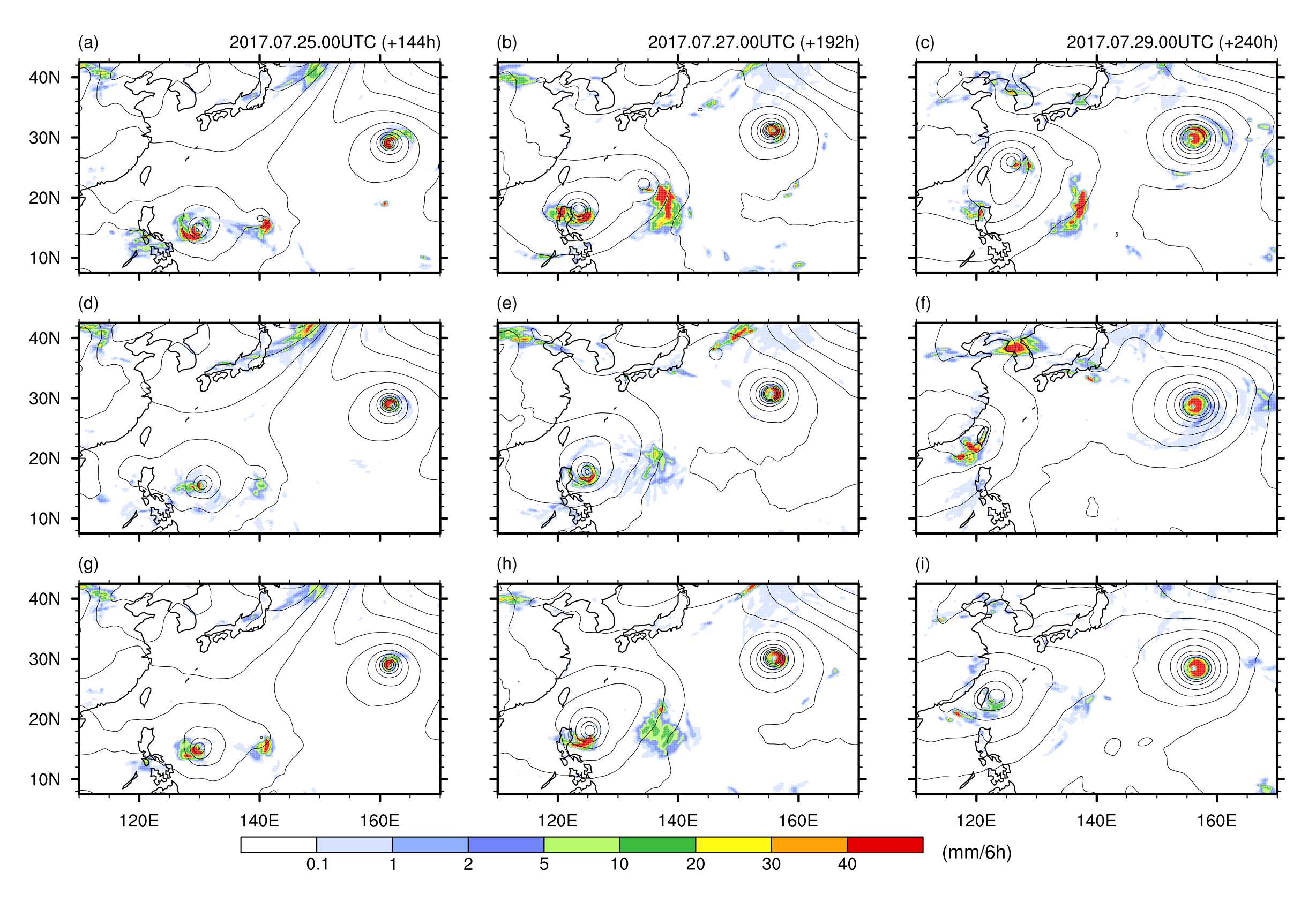
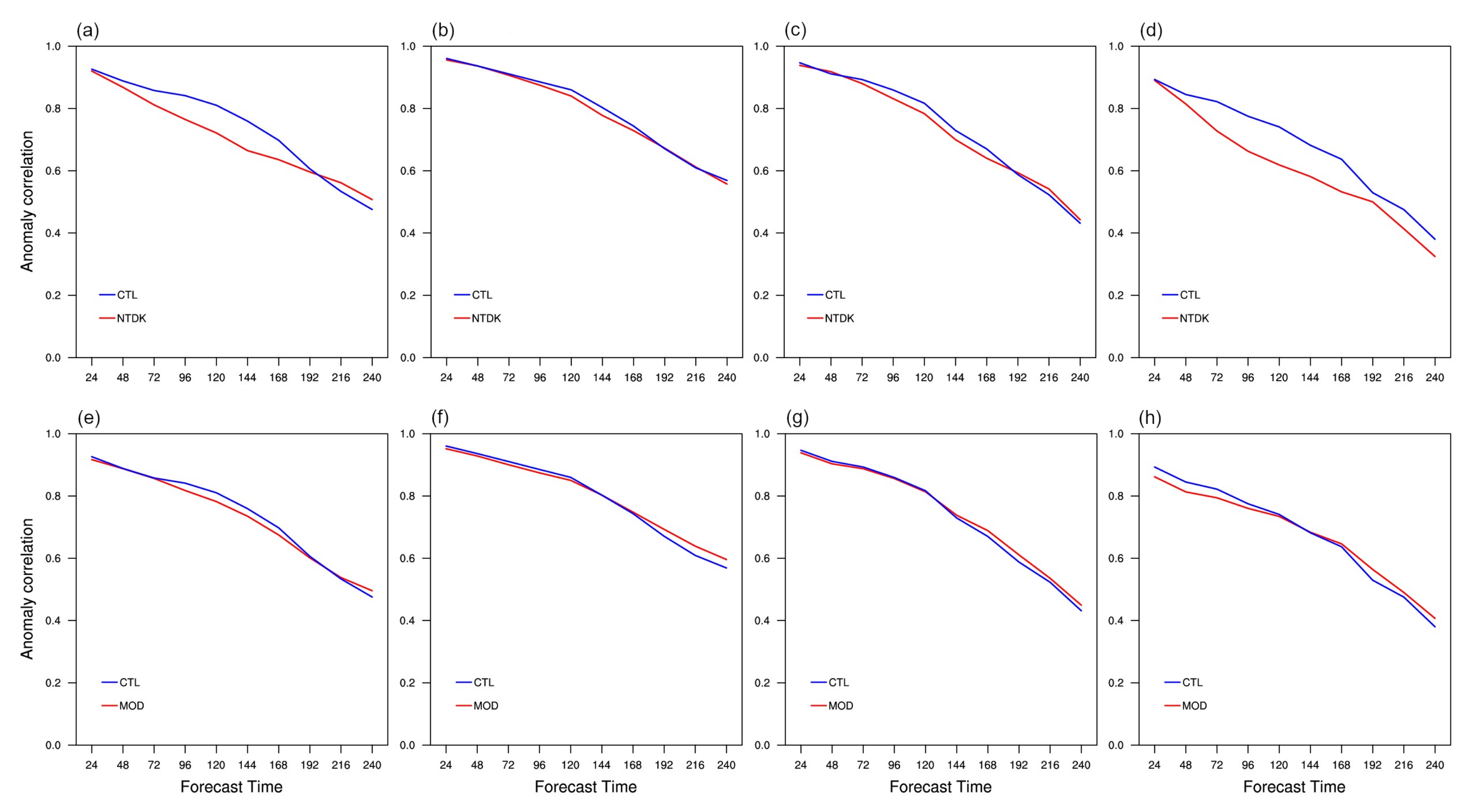
3.3. Impact of Convection Scheme Modification: Medium-Range Forecast Experiments

The impact of the modified entrainment and detrainment rates in the MOD experiment is investigated by also performing twenty 10-day forecast experiments, and the individual and averaged results are presented in Figure 9. The averaged fraction of grid columns containing updrafts stronger than 0.5 m s${}^{-1}$ does not increase in the MOD-COARSE experiments, while the averaged fraction in the CTL-COARSE experiments increases with time as in the single-case CTL experiment (Figure 3). The individual fractions in the CTL-COARSE experiments also exhibit a temporally increasing trend. The averaged grid-scale precipitation rate increases with time in the CTL-COARSE experiments, but the increasing trend is less distinct in the MOD-COARSE experiments. The p-value for the averaged grid-scale precipitation rate in the CTL-COARSE and MOD-COARSE experiments is almost zero, illustrating that their difference is statistically significant. This confirms that grid-point storms are well suppressed by the modification of the KSAS scheme in the coarse-resolution forecast experiments. As in the single-case experiments (Figure 8c), the averaged total precipitation rates in the two experiment sets are quite similar in magnitude (1.48 and 1.45 mm 6 h${}^{-1}$) due to the increased convective precipitation in the MOD-COARSE experiments (Figure 9c).

The precipitation forecast fields averaged over the 3-day forecast period during 1–20 July 2017 in the CTL-COARSE experiments and the fields of precipitation rate difference are plotted in Figure 10. The distribution of precipitation in the intertropical convergence zone and along the extratropical storm tracks is well simulated in the CTL-COARSE experiments (Figure 10a,b), but the precipitation over the Indian Ocean and Maritime Continent is underestimated when compared with the TMPA observations (Figure 10c). While the precipitation over the Bay of Bengal and Philippine Sea increases, the precipitation over the Maritime Continent decreases in both the NTDK-COARSE and MOD-COARSE experiments, resulting a larger mean bias there. It is also notable that the new Tiedtke scheme induces less precipitation over the Pacific Ocean, Atlantic Ocean, and Indian Ocean north of 30° S than CTL-COARSE experiments (Figure 10d). On the other hand, the MOD-COARSE experiments tend to produce more precipitation over the western Atlantic Ocean and northern Indian Ocean as well as western tropical Pacific Ocean than the CTL-COARSE experiments (Figure 10e).

To check more on overall performance, the anomaly correlations of geopotential height are analyzed (Figure 11). While there are little differences in the anomaly correlations of geopotential height between the CTL-COARSE and NTDK-COARSE experiments in the Northern and Southern extratropical regions (not shown), the anomaly correlations of the NTDK-COARSE experiments in the tropical region (20° S–20° N) are much lower than those of the CTL-COARSE experiments, especially at the 100- and 850-hPa levels (Figure 11a–d). The anomaly correlations of the MOD-COARSE experiments in the tropics are generally lower than those of the CTL-COARSE experiments in the early forecast period and vice versa in the late forecast period. The differences in the anomaly correlations of geopotential height between the CTL-COARSE and MOD-COARSE experiments are smaller than the differences between the CTL-COARSE and NTDK-COARSE experiments (Figure 11e–h). These complicated evaluation results highlight that the new Tiedtke scheme nor the modified KSAS scheme guarantee a better performance when implemented in the KIM although the two schemes can suppress the grid-point storms.

4. Summary and Concluding Remarks

The deep convection scheme in the KIM was tentatively modified to suppress grid-point storms in the boreal summertime in the Western Pacific Ocean. Before the modification, a 10-day control simulation and a five-day simulation starting from the five-day control integration but with the new Tiedtke scheme (instead of the default KSAS scheme) were conducted and compared with each other. The heating and drying tendencies in the simulation with the new Tiedtke scheme are stronger than those in the control simulation, and the generation of grid-point storms is suppressed. Thus, the entrainment and detrainment rates in the KSAS scheme were reduced to have stronger heating and drying tendencies, and the same summertime case was simulated using the modified scheme. While one grid-point storm emerges around the TC Nesat before the end of the five-day integration and strengthens with time in the control simulation, the grid-point storm weakens and the grid-scale precipitation decreases in the simulation with the modified scheme. The suppression of the grid-point storm with the modified scheme improves the track forecast of the TC Nesat. Similar responses were found in the twenty coarse-resolution forecast experiments, illustrating that the modification of the entrainment and detrainment rates of the convection scheme could successfully suppress grid-point storms in the KIM.

This study illustrated the possibility of suppressing unrealistic moist disturbances by simply modifying the deep convection scheme. The modified KSAS scheme, however, does not significantly improve overall performance (e.g., mean bias, anomaly correlation), so more re-tuning is required. Furthermore, the impacts of the modification on other cases (e.g., boreal wintertime cases and other TCs) and its impacts on other physical processes need to be investigated to improve the stability and performance of the KIM. In addition to modifying entrainment and detrainment rates, heating and drying tendencies can be controlled by changing the convective adjustment time scale or the background cloud work function. The tendencies can also be controlled by modifying the microphysical parts in the cumulus convection schemes. For example, changing the amount of rain evaporation can affect convective instability and precipitation, and this requires more study for further improvements. Note that this kind of modification can suppress unrealistic grid-point storms but does not guarantee a better performance (e.g., higher skill scores). Thus, an extensive evaluation should be done along with careful modifications to improve a numerical forecasting model.

References

1. Bechtold, P.; Köhler, M.; Jung, T.; Doblas-Reyes, F.; Leutbecher, M.; Rodwell, M.J.; Vitart, F.; Balsamo, G. Advances in simulating atmospheric variability with the ECMWF model: From synoptic to decadal time-scales. Q. J. R. Meteorol. Soc. 2008, 134, 1337–1351. [Google Scholar] [CrossRef]
2. Han, J.; Pan, H.L. Revision of convection and vertical diffusion schemes in the NCEP Global Forecast System. Weather Forecast. 2011, 26, 520–533. [Google Scholar] [CrossRef]
3. Zhang, D.L.; Hsie, E.Y.; Moncrieff, M.W. A comparison of explicit and implicit predictions of convective and stratiform precipitating weather systems with a meso-β-scale numerical model. Q. J. R. Meteorol. Soc. 1988, 114, 31–60. [Google Scholar] [CrossRef]
4. Molinari, J.; Dudek, M. Parameterization of convective precipitation in mesoscale numerical models: A critical review. Mon. Weather Rev. 1992, 120, 326–344. [Google Scholar] [CrossRef] [Green Version]
5. Hong, S.Y.; Kwon, Y.C.; Kim, T.H.; Kim, J.E.E.; Choi, S.J.; Kwon, I.H.; Kim, J.; Lee, E.H.; Park, R.S.; Kim, D.I. The Korean Integrated Model (KIM) system for global weather forecasting. Asia-Pac. J. Atmos. Sci. 2018, 54, 267–292. [Google Scholar] [CrossRef]
6. Choi, S.J.; Giraldo, F.X.; Kim, J.; Shin, S. Verification of a non-hydrostatic dynamical core using the horizontal spectral element method and vertical finite difference method: 2-D aspects. Geosci. Model Dev. 2014, 7, 2717–2731. [Google Scholar] [CrossRef] [Green Version]
7. Choi, S.J.; Hong, S.Y. A global non-hydrostatic dynamical core using the spectral element method on a cubed-sphere grid. Asia-Pac. J. Atmos. Sci. 2016, 52, 291–307. [Google Scholar] [CrossRef]
8. Song, H.J.; Kwon, I.H. Spectral transformation using a cubed-sphere grid for a three-dimensional variational data assimilation system. Mon. Weather Rev. 2015, 143, 2581–2599. [Google Scholar] [CrossRef]
9. Kang, J.H.; Chun, H.W.; Lee, S.; Ha, J.H.; Song, H.J.; Kwon, I.H.; Han, H.J.; Jeong, H.; Kwon, H.N.; Kim, T.H. Development of an observation processing package for data assimilation in KIAPS. Asia-Pac. J. Atmos. Sci. 2018, 54, 303–318. [Google Scholar] [CrossRef]
10. Baek, S. A revised radiation package of G-packed McICA and two-stream approximation: Performance evaluation in a global weather forecasting model. J. Adv. Model. Earth Syst. 2017, 9, 1628–1640. [Google Scholar] [CrossRef]
11. Park, R.S.; Chae, J.H.; Hong, S.Y. A revised prognostic cloud fraction scheme in a global forecasting system. Mon. Weather Rev. 2016, 144, 1219–1229. [Google Scholar] [CrossRef]
12. Koo, M.S.; Baek, S.; Seol, K.H.; Cho, K. Advances in land modeling of KIAPS based on the Noah Land Surface Model. Asia-Pac. J. Atmos. Sci. 2017, 53, 361–373. [Google Scholar] [CrossRef]
13. Koo, M.S.; Choi, H.J.; Han, J.Y. A parameterization of turbulent-scale and mesoscale orographic drag in a global atmospheric model. J. Geophys. Res. Atmos. 2018, 123, 8400–8417. [Google Scholar] [CrossRef]
14. Kim, E.J.; Hong, S.Y. Impact of air-sea interaction on East Asian summer monsoon climate in WRF. J. Geophys. Res. 2010, 115. [Google Scholar] [CrossRef]
15. Lee, E.; Hong, S.Y. Impact of the sea surface salinity on simulated precipitation in a global numerical weather prediction model. J. Geophys. Res. Atmos. 2019, 124, 719–730. [Google Scholar] [CrossRef]
16. Shin, H.H.; Hong, S.Y. Representation of the subgrid-scale turbulent transport in convective boundary layers at gray-zone resolutions. Mon. Weather Rev. 2015, 143, 250–271. [Google Scholar] [CrossRef]
17. Lee, E.H.; Lee, E.; Park, R.; Kwon, Y.C.; Hong, S.Y. Impact of turbulent mixing in the stratocumulus-topped boundary layer on numerical weather prediction. Asia-Pac. J. Atmos. Sci. 2018, 54, 371–384. [Google Scholar] [CrossRef]
18. Choi, H.J.; Hong, S.Y. An updated subgrid orographic parameterization for global atmospheric forecast models. J. Geophys. Res. Atmos. 2015, 120, 12445–12457. [Google Scholar] [CrossRef]
19. Choi, H.J.; Han, J.Y.; Koo, M.S.; Chun, H.Y.; Kim, Y.H.; Hong, S.Y. Effects of non-orographic gravity wave drag on seasonal and medium-range predictions in a global forecast model. Asia-Pac. J. Atmos. Sci. 2018, 54, 385–402. [Google Scholar] [CrossRef]
20. Hong, S.Y.; Dudhia, J.; Chen, S.H. A revised approach to ice microphysical processes for the bulk parameterization of clouds and precipitation. Mon. Weather Rev. 2004, 132, 103–120. [Google Scholar] [CrossRef]
21. Bae, S.Y.; Hong, S.Y.; Lim, K.S.S. Coupling WRF double-moment 6-class microphysics schemes to RRTMG radiation scheme in weather research forecasting model. Adv. Meteorol. 2016, 2016, 5070154. [Google Scholar] [CrossRef]
22. Kim, S.Y.; Hong, S.Y. The use of partial cloudiness in a bulk cloud microphysics scheme: Concept and 2D results. J. Atmos. Sci. 2018, 75, 2711–2719. [Google Scholar] [CrossRef]
23. Han, J.Y.; Hong, S.Y.; Lim, K.S.S.; Han, J. Sensitivity of a cumulus parameterization scheme to precipitation production representation and its impact on a heavy rain event over Korea. Mon. Weather Rev. 2016, 144, 2125–2135. [Google Scholar] [CrossRef]
24. Kwon, Y.C.; Hong, S.Y. A mass-flux cumulus parameterization scheme across gray-zone resolutions. Mon. Weather Rev. 2017, 145, 583–598. [Google Scholar] [CrossRef]
25. Han, J.Y.; Hong, S.Y. Precipitation forecast experiments using the weather research and forecasting (WRF) model at gray-zone resolutions. Weather Forecast. 2018, 33, 1605–1616. [Google Scholar] [CrossRef]
26. Han, J.Y.; Hong, S.Y.; Kwon, Y.C. The performance of a revised simplified Arakawa–Schubert (SAS) convection scheme in the medium-range forecasts of the Korean Integrated Model (KIM). Weather Forecast. 2020, 35, 1113–1128. [Google Scholar] [CrossRef] [Green Version]
27. Copernicus Climate Change Service (C3S). ERA5: Fifth Generation of ECMWF Atmospheric Reanalyses of the Global Climate. Available online: https://cds.climate.copernicus.eu/cdsapp#!/home (accessed on 2 January 2019).
28. Huffman, G.J.; Bolvin, D.T.; Nelkin, E.J.; Wolff, D.B.; Adler, R.F.; Gu, G.; Hong, Y.; Bowman, K.P.; Stocker, E.F. The TRMM multisatellite precipitation analysis (TMPA): Quasi-global, multiyear, combined-sensor precipitation estimates at fine scales. J. Hydrometeorol. 2007, 8, 38–55. [Google Scholar] [CrossRef]
29. Tiedtke, M. A comprehensive mass flux scheme for cumulus parameterization in large-scale models. Mon. Weather Rev. 1989, 117, 1779–1800. [Google Scholar] [CrossRef] [Green Version]
30. Bechtold, P.; Semane, N.; Lopez, P.; Chaboureau, J.P.; Beljaars, A.; Bormann, N. Representing equilibrium and nonequilibrium convection in large-scale models. J. Atmos. Sci. 2014, 71, 734–753. [Google Scholar] [CrossRef] [Green Version]
31. Zhang, C.; Wang, Y.; Hamilton, K. Improved representation of boundary layer clouds over the Southeast Pacific in ARW-WRF using a modified Tiedtke cumulus parameterization scheme. Mon. Weather Rev. 2011, 139, 3489–3513. [Google Scholar] [CrossRef] [Green Version]
Figure 1. Fields of the six-hourly precipitation rate at 0000 UTC on July (a) 21, (b) 23, (c) 25, (d) 27, and (e) 29, 2017 from the TMPA observations and the same fields from the CTL experiment (fj). Sea-level pressure contours (4 hPa interval) from the ERA5 reanalysis data and CTL experiment are added to show synoptic systems with the precipitation rate fields. The area shown in Figure 2a is indicated with a rectangle with blue solid lines in (h).
Atmosphere 12 01194 g001
Figure 2. (a) Horizontal distribution of the six-hourly grid-scale precipitation rate (shaded; mm 6 h 1 ) and (b) the vertical distribution of the mixing ratio of rain and snow (shaded; g kg 1 ) across the gray transect in (a) at 1200 UTC on 24 July 2017 from the CTL experiment. Sea-level pressure contours (4 hPa interval) are added in (a), and contours of vertical velocity of 0.4 m s 1 are added in (b).
Atmosphere 12 01194 g002
Figure 3. Time series of (a) the fraction of grid columns where the maximum vertical velocity is larger than 1 m s 1 and (b) the fraction of grid columns where the six-hour accumulated grid-scale precipitation amount is larger than 80 mm in the selected domain (100° E–160° W, 0–50° N) from the CTL (black dashed), NTDK (blue dotted), and MOD (red solid) experiments.
Atmosphere 12 01194 g003
Figure 4. Vertical profiles of (a) the heating and (b) moistening tendencies averaged over the selected domain (100° E–160° W, 0–50° N) and over the period from 0000 UTC on 24 July to 0000 UTC on 25 July 2017 from the CTL (black dashed), NTDK (blue dotted), and MOD (red solid) experiments. Note that the tendencies from the GFS shallow convection scheme are included in the CTL and MOD profiles.
Atmosphere 12 01194 g004
Figure 5. (a) Horizontal distribution of the six-hourly grid-scale precipitation rate (shaded; mm 6 h 1 ) and (b) the vertical distribution of the mixing ratio of rain and snow (shaded; g kg 1 ) across the gray transect in (a) at 1200 UTC on 24 July 2017 from the MOD experiment. Sea-level pressure contours (4 hPa interval) are added in (a), and contours of vertical velocity of 0.4 m s 1 are added in (b).
Atmosphere 12 01194 g005
Figure 6. Fields of the six-hourly grid-scale precipitation rate (shaded; mm 6 h 1 ) at 0000 UTC on July (a) 25, (b) 27, and (c) 29, 2017 in the CTL experiment, and the same fields in the NTDK experiment (df) and in the MOD experiment (gi). Sea-level pressure contours (4 hPa interval) are presented with the precipitation rate fields.
Atmosphere 12 01194 g006
Figure 7. (a) Trajectories of the TC Nesat and (b) time series of the minimum sea-level pressure from KMA (green) and CTL (black), NTDK (blue), and MOD (red) experiments.
Atmosphere 12 01194 g007
Figure 8. Time series of the six-hourly (a) grid-scale, (b) convective, and (c) total precipitation rates averaged over the selected domain (100° E–160° W, 0–50° N) from the CTL (black dashed), NTDK (blue dotted), and MOD (red solid) experiments. The dotted gray line in (c) shows the averaged TMPA precipitation rate.
Atmosphere 12 01194 g008
Figure 9. Time series of (a) the fraction of grid columns where the maximum vertical velocity is larger than 0.5 m s 1 , (b) the six-hourly grid-scale precipitation rate, and (c) the six-hourly total precipitation rate averaged over the selected domain (100° E–160° W, 0–50° N) from the CTL-COARSE (black) and MOD-COARSE (brown) experiments. Thin and thick lines indicate individual and averaged results, respectively.
Atmosphere 12 01194 g009
Figure 10. Global distribution of the precipitation rate (mm day 1 ) from the (a) TMPA observations and (b) CTL-COARSE experiments averaged over the 3-day forecast period during 1–20 July 2017 and the precipitation rate differences between the (c) CTL-COARSE and TMPA, (d) NTDK-COARSE and CTL-COARSE experiments, and (e) MOD-COARSE and CTL-COARSE experiments.
Atmosphere 12 01194 g010
Figure 11. Anomaly correlation for forecasts of the (a) 100-, (b) 250-, (c) 500-, and (d) 850-hPa geopotential height in the tropics (20° S–20° N) against the ERA5 analysis data during 1–20 July 2017 from the CTL-COARSE (blue) and NTDK-COARSE (red) experiments and the same anomaly correlation from the CTL-COARSE (blue) and MOD-COARSE (red) experiments (eh).
Atmosphere 12 01194 g011
Publisher’s Note: MDPI stays neutral with regard to jurisdictional claims in published maps and institutional affiliations.