Abstract
To assess the quality of the retrieved products from ground-based microwave radiometers, the “clear-sky” Level-2 data (LV2) products (profiles of atmospheric temperature and humidity) filtered through a radiometer in Beijing during the 24 months from January 2010 to December 2011 were compared with radiosonde data. Evident differences were revealed. Therefore, this paper investigated an approach to calibrate the observed brightness temperatures by using the model-simulated brightness temperatures as a reference under clear-sky conditions. The simulation was completed with a radiative transfer model and National Centers for Environmental Prediction final analysis (NCEP FNL) data that are independent of the radiometer system. Then, the least-squares method was used to invert the calibrated brightness temperatures to the atmospheric temperature and humidity profiles. A comparison between the retrievals and radiosonde data showed that the calibration of the brightness temperature observations is necessary, and can improve the inversion of temperature and humidity profiles compared with the original LV2 products. Specifically, the consistency with radiosonde was clearly improved: the correlation coefficients are increased, especially, the correlation coefficient for water vapor density increased from 0.2 to 0.9 around the 3 km height; the bias decreased to nearly zero at each height; the RMSE (root of mean squared error) for temperature profile was decreased by more than 1 degree at most heights; the RMSE for water vapor density was decreased from greater than 4 g/m3 to less than 1.5 g/m3 at 1 km height; and the decrease at all other heights were also noticeable. In this paper, the evolution of a temperature inversion process is given as an example, using the high-temporal-resolution brightness temperature after quality control to obtain a temperature and humidity profile every two minutes. Therefore, the characteristics of temperature inversion that cannot be seen by conventional radiosonde data (twice daily) were obtained by radiometer. This greatly compensates for the limited temporal coverage of radiosonde data. The approach presented by this paper is a valuable reference for the reprocessing of the historical observations, which have been accumulated for years by less-calibrated radiometers.
1. Introduction
Data products such as atmospheric temperature and humidity profiles, referred to as Level-2 data and abbreviated as LV2, are the retrievals from brightness temperatures measured with ground-based microwave radiometers (referred to as Level-1 data, abbreviated as LV1, and denoted as TBM in this paper). They provide continuous information for the monitoring and early warning of severe weather [1,2,3]. Many studies have shown that these data play an important role in the analysis of atmospheric stability, weather forecasting, weather modification, and other research and operations [4,5,6,7,8,9,10,11,12]. Chan [13] analyzed the precipitation and K-index (an indicator for atmospheric stability) for two severe convection weather processes in Hong Kong and found that a microwave radiometer can provide useful information for weather prediction, though there were certain differences between the microwave radiometer observations and radiosonde data. Sánchez et al. [14] compared the temperature and water vapor density profiles of a 35-channel ground-based microwave radiometer in Madrid with radiosonde data, and concluded that the linear relationship between the two datasets can be used for data quality control. Liu [15] explored the influence factors (such as altitude, season, and cloud) on the difference between the temperature profiles measured by a ground-based 12-channel microwave radiometer and the radio sounding by comparing the brightness temperatures measured by the radiometer with the simulated data. Liu et al. [16] used sounding data from Beijing to conduct neural network training for all four seasons, carried out a numerical test on the inversion ability of the trained network, and evaluated the inversion accuracy. Xu et al. [17] used same-site radiosonde data to verify the temperature, relative humidity, and water vapor density from a microwave radiometer, and found that the profiles from the microwave radiometer had a good positive correlation with the radiosonde, while the correlation coefficient for relative humidity was greatly affected by the weather. Guo et al. [18] collected 170 samples of vertical sounding (of which 30 are for fog occurrence) during 11 fog weather processes to verify the temperature, water vapor density, and relative humidity retrievals from a 35-channel microwave radiometer. A comparison between the model-simulated brightness temperatures and the brightness temperatures measured by the microwave radiometer showed that the simulated brightness temperatures were less than the measured on average, but the temperature and relative humidity retrieved were closely consistent with the tethered balloon during the development and evolution of the fog.
Now that LV2 data are obtained via a retrieval calculation of brightness temperatures measured by radiometer, if the LV1 data appear to be distinctly different from the simulated, LV2 obtained from the retrieval are bound to be greatly inconsistent with radiosonde (as well as reanalysis data for a numerical model output). To this end, studies have emphasized the need for quality control before applying measured brightness temperature data [19,20,21]. For example, it was found, based on a two-year data study, that a time segmentation phenomenon existed in the “clear-sky” [22] LV1 data of a radiometer in Beijing. Different segments had different systematic deviations as compared with the simulation data. For this reason, segmentation bias correction (and environmental impact correction) was proposed and implemented, which improved the time continuity within the two-year observational data and the consistency with the simulation data. This provided a quality guarantee for the LV1 data to be further used for the inversion of temperature and humidity profiles.
The present study used the radiometer at Beijing as an example to present an approach to calibrate the observed brightness temperatures by using the model-simulated brightness temperatures as a reference under clear-sky conditions. Firstly, a method named the “three-channel method” is given for brightness temperature classification to filter out the clear-sky cases. Secondly, the LV2 products for “clear sky” in a two-year period were compared with radiosonde data so that the quality of the LV2 products was evaluated according to standard practice [13,14,15,16,17,18] and the low-quality features of LV2 and the problems in TBM were revealed. Then, to improve the LV2 data quality, a method for TBM correction was presented based on using the brightness temperature value calculated by the radiation transfer model and NCEP FNL (National Centers for Environmental Prediction final analysis) profiles [23,24,25]. The results from the TBM correction, denoted as TBO, was adopted to retrieve the profiles of temperature and humidity based on the least-square regression. Finally, by comparing the retrieved atmospheric temperature and humidity profiles with radiosonde observations (RAOB), the effect of brightness temperature data correction on improving the consistency between LV2 data and radiosonde data was verified.
2. Data and Clear-Sky Samples
2.1. Data
The radiometer data used for this paper were the LV1 and LV2 products from January 2010 to December 2011 from a radiometer system in Beijing. The channel and frequency settings of the radiometer are shown in the first two columns of Table 1. The right four columns in Table 1 show the brightness temperatures measured (TBM), simulated (TBC), and corrected (TBO) by this study for four examples. The four examples will be discussed further in Section 3 as case analyses.

Table 1.
The radiometer channel frequency used for atmospheric temperature and humidity and a comparison of brightness temperatures before and after correction.
The time-matched radiosonde data for the Beijing RAOB Station were downloaded from Wyoming University’s website (http://weather.uwyo.edu/upperair/sounding.html, accessed 24 September 2014) and used as the “truth” for the evaluation. The atmospheric temperature and humidity data provided by NCEP FNL were input into the radiative transfer model [26], and the brightness temperatures were output after thorough radiative transfer calculation, which are denoted as TBC in this article [27].
2.2. Scheme to Obtain the Clear-Sky Samples
The term “clear sky” for classification of atmospheric profiles can be defined as relative humidity being less than 85% at any height for the Beijing district according to literature [22]. However, in order to classify the brightness temperature data, we present a method based on Channels 2, 7, and 10 in Table 1 because the three channels are most sensitive to cloud height, thickness, and water concentration according to sensitivity analyses. The method, named the “three-channel method”, is described as the following steps.
- (1)
- Based on the relevant cloud physics literature [28,29], clouds are divided into ten types, with each cloud type having four possible cloud base heights, four thicknesses, and five possible cloud water concentrations, so that a parameter space comprising 800 possible cloud parameter combinations was constructed, as shown in Table 2.
Table 2. The 800 possible combinations of cloud parameter values based on the literature.
- (2)
- The 1976 US standard atmosphere was adopted and a relative humidity of 95% was set at each height in cloud layers as defined in Table 2 to form a cloudy layer for the simulation calculation of the cloud contribution to the brightness temperature measurement.
- (3)
- The sensitivity of the cloud contribution in each channel to cloud water concentration and cloud thickness is analyzed for each channel, which gives the result that Channels 2, 7, and 10 are the best channels for cloud identification, and the estimated water concentration and cloud thickness based on regression for the three channels are noted as and , respectively. The standard deviation of residuals for each channel is also obtained from regression analysis, so that one has and , respectively.
- (4)
- The weighted averagewould combine and together to give a better estimation of the water concentration and cloud thickness. The weights in Equation (1a,b) are the reciprocal of the standard deviation and .
- (5)
- If the cloud parameters inversed from Equation (1a,b) are close to 0, it can be judged that the corresponding time is “clear-sky” time.
According to this method, the final sample size of “clear sky” in Beijing’s two-year data is 594, considering that the radio sounding is performed twice a day.
3. Error Statistics and Case Analysis of the LV2 Product
In this study, the clear-sky sample with 594 cases was randomly separated into two subsamples. The subsample with 60 cases was adopted as quality test samples, which were compared with RAOB for error analysis, and the subsample with the remaining 534 cases was adopted for regression to set up the inversion model for retrieving temperature and humidity profiles from the brightness temperatures.
The results from the quality test samples are shown in Figure 1 and Figure 2. The ordinate of these figures uses piecewise linearity to make it easier to see the vertical variation of the statistics in the lower layers of the atmosphere. The maximum height is set to 10 km according to the specifications of the radiometer system. The “error” is defined as the value of the retrievals minus RAOB, the bias is the average of the errors, and the RMSE is the root of mean squared error.
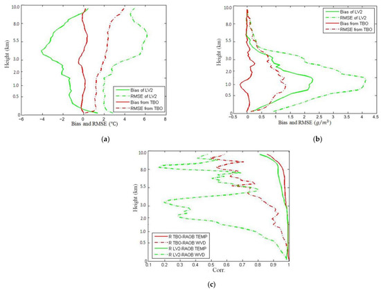
Figure 1.
Statistics of temperature and humidity profiles as compared with radiosonde observations (RAOB) (green line, LV2; red line, ). (a) bias and root of mean squared error (RMSE) for temperature; (b) bias and RMSE for humidity; (c) correlation coefficients.
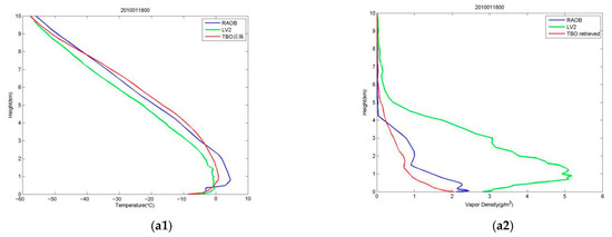
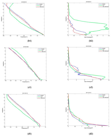
Figure 2.
Four typical cases for comparison between the retrieved temperature and humidity profiles with RAOB. Blue lines for RAOB; green lines for LV2; and red lines for . (a1) Case 1: 2010011800 temperature; (a2) Case 1: 2010011800 water vapor density; (b1) Case 2: 2010020212 temperature; (b2) Case 2: 2010020212 water vapor density; (c1) Case 3: 2010072400 Temperature; (c2) Case 3: 2010072400 water vapor density; (d1) Case 4: 2011123112 temperature; (d2) Case 4: 2011123112 water vapor density.
Figure 1 shows the statistics of the errors and correlation. One can see the following.
- (1)
- From Figure 1a, the LV2 temperature bias was negative overall (solid green line), with a bias of −4 °C at the height of 4.4 km, implying that the retrievals from the radiometer system provided by the manufacture are generally cooler than the RAOB, and the RMSE of the temperature (green dotted line) was greater than 2 °C at each level, even reaching 6 °C at the height of 5.5 km.
- (2)
- Figure 1b shows that the bias of the LV2 water vapor density was positive overall, implying that the retrievals from the radiometer system are generally moister than the RAOB. Further, it must be pointed out that the bias is as large as 2.3 g/m3 near the height of 1.0 km (solid green line) and the RMSE (dotted green line) was 4.0 g/m3, the same order as in the common air.
- (3)
- From Figure 1c, the correlation coefficient between the LV2 temperature and the RAOB, as shown by the solid green line, was close to 1 below 3 km and no less than 0.8 above, but the correlation coefficient between the LV2 water vapor density and the RAOB, as shown by the dotted green line, decreased quickly from 1 at the ground to less than 0.3 at the 2 km height.
Figure 2 is for case comparison. The four cases given in Table 1 are shown in Figure 2 in chronological order. Their times are sequentially 2010011800, representing 0000 UTC (0800 BT for local time) on 18 January 2010, and 2010020212, 2010072400, and 2011123112, respectively. Three of the four cases are from winter and one is from summer, because LV2 is even worse in winter than in summer after we review all of the cases from the two years. It is well-known that Beijing is cool and dry in winter, and a temperature inversion layer would occur due to the diurnal variation of the surface temperature [30]. The temperature inversion layer increases the difficulty of temperature remote sensing. The difficulty for humidity remote sensing is the dry feature in winter, and the output from LV2 is often wetter than the RAOB.
Figure 2a,b,d shows that LV2 lines (green) are notably different from the RAOB for both temperature and humidity. One can see that Figure 2(a1) is a typical boundary layer temperature inversion. The height and severity of the inversion layer revealed by LV2 (green line) are lower and weaker. LV2 in Figure 2(b1,d1) are close to the RAOB near the ground but too cool in middle troposphere, and the tropopause heights defined by LV2 are also lower than the RAOB [31]. As shown in Figure 2(a2,b2), LV2 almost always presents an erroneous “moisture layer” suspended in midair, and the maximum humidity value is much larger than the RAOB. Figure 2(d2) shows that LV2 indicated as too dry at 1200 UTC on the last day of 2011 as compared with the RAOB.
From Figure 2(a2), the RAOB indicated that the water vapor density was 2 g/m3 at the ground and decreased with height, while the water vapor density of LV2 was characterized by an erroneous moisture inversion layer. The water vapor density at 1 km height was as high as 5 g/m3, obviously larger than in the RAOB.
From Figure 2(b1), the RAOB indicated that the tropopause height was close to 10 km, while LV2 produced a lower tropospheric height of less than 9 km. From Figure 2(b2), the RAOB indicated that the water vapor density decreased from 1.6 g/m3 at the ground with increasing altitude, while LV2 showed the same water vapor density characteristics as in Figure 1(b1), with an erroneous, distinct moisture inversion layer.
Figure 2c is for a typical summer in Beijing. The air temperature near the ground is approximately 30 °C and the water vapor density is approximately 20 g/m3. LV2 shown in Figure 2c were not too bad in summer but still differed greatly from the RAOB. For example, as shown in Figure 2(c2), water vapor density decreased with height in the lower layer according to the RAOB, while LV2 showed a moisture inversion layer.
From Figure 2(d1), the RAOB indicated that there was weak inversion near the ground, while according to LV2 no inversion existed, the whole atmospheric temperature was low, and the temperature at the height of 5 km was lower than 10 °C. Finally, from Figure 2(d2), the RAOB indicated that the water vapor density decreased from 2.9 g/m3 at the ground with increasing height, but LV2 said the water vapor density near the ground was 1.5 g/m3, only half of the RAOB.
4. Correction of Brightness Temperature from TBM to TBO
As seen above, the difference between LV2 and RAOB was obvious. Previous studies [19,20,21] revealed that the measured brightness temperature value (TBM) and the calculated value (TBC) were greatly different. To this end, the following procedure was performed on the subsample with the 534 clear-sky cases to set up a relationship for the TBM correction.
- (1)
- The simulated value of the brightness temperature was calculated by using a radiation transfer model and the atmospheric profiles in the NCEP FNL, and recorded as TBC.
- (2)
- A fitting relationship between TBC and TBM was established as follows:where is the surface temperature (representing the correction for the influence from the environment temperature of the radiometer), and the coefficients a, b, and c were obtained by regression analysis.
- (3)
- The corrected value of brightness temperature would be obtained bywhere the coefficients a, b, and c are just from the last step.
All the 60 cases in the subsample for the quality test were processed for brightness temperature correction according to Equation (3). Taking the four cases given in Figure 2 as an example, the TBM, TBC, and TBO values of each channel are shown in Table 1. It can be seen that TBM may differ from TBO by a few Kelvin, and the correction of brightness temperature was obvious. Therefore, TBO was used to retrieve the temperature and humidity profiles, and the consistency with RAOB was expected to be improved. This expectation is investigated and discussed in the following section.
5. Error Statistics and Case Analysis of the Profiles Retrieved from TBO
As long as TBO for the test samples was completed, the subsample with the 534 clear-sky cases was also processed for brightness temperature correction according to Equation (3). Then the subsample was used as training samples to establish the relationship for inversing the brightness temperature to the temperature and humidity profiles. The retrieval calculations in this paper adopted the simple and straightforward least-squares method [26], which is briefly described as follows:
Let the vector be the brightness temperature of the K channels,
and the regression equation is
where C is the regression coefficient matrix and can be obtained through regression analysis by using a regression sample (of sample size M = 534) of both and based on the least-squares method to give
In the calculation of the regression coefficient matrix C, is the temperature and water vapor density provided by the NCEP FNL data, and is the TBO. In the retrieval calculation for the quality test subsample, the calculated by Equation (5) is the temperature and humidity profile obtained by the retrieval, which is denoted as in the study.
The for the four cases is shown in Figure 2 as red lines. One can see that: In Case 1 (Figure 2a), the top height of the inversion layer shown by the (red line in Figure 2(a1)) was at 1 km, which was consistent with the RAOB, and the temperature at 1 km was obviously close to the RAOB; the water vapor density line (red line in Figure 2(a2)), although “dry”, was closer to the RAOB than the LV2.
In Case 2 (Figure 2b), the temperature (red line in Figure 2(b1)) coincided with the RAOB at almost all heights, especially the tropopause height; the water vapor density line (red line in Figure 2(b2)) showed an advantage over the LV2.
In Case 3 (Figure 2c), the trend of the temperature line was consistent with the RAOB, while the LV2 was warmer at the ground and above (Figure 2(c1)); the water vapor density line eliminated the mistake of the LV2 around the 1 km height (Figure 2(c2)).
In Case 4 (Figure 2d), the temperature line better reflected the near-surface weak inversion and tropopause characteristics; and the water vapor density value was 3 g/m3 at the ground, which was consistent with RAOB, whereas LV2 was only 1.5 g/m3.
The statistical results of in the quality test sample are given in Figure 1 as red line. The bias of the temperature at all heights was almost zero (Figure 1a), and the RMSE was obviously reduced to less than 2 °C below 5 km. From Figure 1b, the bias of the water vapor density was also almost zero, and the RMSE at 1 km shows its maximum but still less than 1.5 g/m3, which was much better than the LV2 (4 g/m3). Figure 1c shows that the correlation between the and the RAOB for temperature was better than the LV2, especially over 3 km. The correlation between the and RAOB for water vapor density was as large as 0.9 at the height of 3 km, much better than 0.2 for the LV2.
Therefore, one can say that the correction of the brightness temperature data before the inversion calculation can effectively improve the consistency between the retrieval results and RAOB data.
6. Retrieval Analysis of a Remotely Sensed Inversion Layer Process
It is well-known that near-ground temperature inversion in Beijing occurs often in winter. Mostly, the inversion grows gradually in the afternoon due to the decreasing surface temperature because of the sunset, and weakens and disappears gradually the next morning due to the increasing surface temperature because of the sunrise. A process like this can be well-observed continuously with a ground-based microwave radiometer. Take 18 December 2010 as an example to analyze the high temporal resolution temperature and humidity profile characteristics within 12 h during 0000–1200 UTC (0800–2000 BT). The weather was clear and breezy with no sustained wind direction. The temperature and humidity profiles at 0800 and 2000 BT from RAOB are shown in Figure 3 as blue lines. Only the information below 3 km is plotted in order to better see the ine height of 0.8 km and fell down to 0.3 km at 2000 BT according to RAOBversion layer. It can be seen that the inversion layer top at 0800 BT was near th. Obviously, such a 12-h interval data does not show the evolution features within the 12 h.
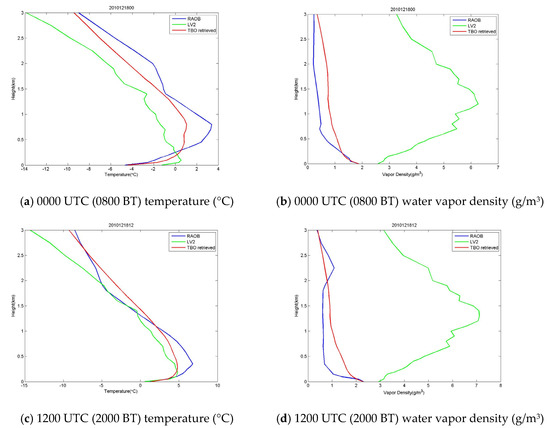
Figure 3.
Temperature and humidity profiles on 18 December 2010, with intervals of 12 h: (a) 0000 UTC temperature; (b) 0000 UTC water vapor density; (c) 1200 UTC temperature; (d) 1200 UTC water vapor density.
On the contrary, the advantage of microwave radiometer data is that temperature and humidity profiles can be provided with high temporal resolution. Figure 4 shows 332 TBO profiles of temperature and humidity at two-minute intervals during 0000–1200 UTC (0800–2000 BT), together with the LV2 product. The white, double-dotted lines indicate the top position of the inversion layer for either the temperature or the humidity. Obviously the TBO is more reliable than the LV2 according to Figure 3, showing that the TBO is closer to the RAOB than the LV2. One can see the following:
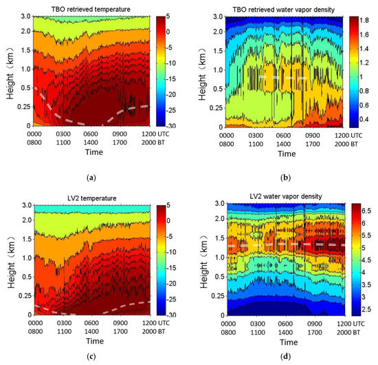
Figure 4.
Temperature and humidity profiles with a 2-min resolution during 0000–1200 UTC (0800–2000 BT) on 18 December 2010, supplied by this study as compared with LV2. (a) temperature retrievals from TBO; (b) water vapor density retrieval from TBO; (c) temperature (°C) of LV2; (d) water vapor density (g/m3) of LV2.
- (1)
- During the morning (0800 and 1400 BT), as the ground was heated by the sun, the top of the temperature inversion layer gradually decreased, weakened, and disappeared, as shown Figure 4a. During the afternoon, the ground temperature gradually decreased due to the weakening of solar radiation, and the top of the inversion layer gradually formed, strengthened, and rose.
- (2)
- The water vapor density in the atmosphere decreased substantially with height (Figure 4b). Only when the temperature inversion layer vanished around the period 1100–1600 BT could surface water vapor be transported upward (water vapor density increases gradually at the height of about 1.4 km), forming a weak moisture inversion layer. While the temperature inversion gradually appeared in the afternoon until the next morning, the water vapor transport gradually stopped and returned to a state of decreasing with height.
- (3)
7. Conclusions
Two years of clear-sky product data of a radiometer in Beijing were compared with radiosonde data, and it was found that the correlation between the LV2 and RAOB was small, a bias obviously existed, and the RMSE was large. Since the LV1 data (brightness temperature) of the radiometer are the input data of the LV2 inversion product, this paper suggests that, before applying the brightness temperature data in the inversion calculation, quality control of the measured brightness temperatures based on NCEP FNL data and radiation transfer simulation were performed to obtain the corrected brightness temperatures (TBO). The results showed that, compared with the RAOB, the temperature and humidity profiles obtained by TBO inversion were obviously better than the LV2 products, the error bias and RMSE were notably reduced, and the correlation with the RAOB was greatly improved. More specifically:
- The bias of the temperature and humidity profile obtained by TBO inversion was reduced almost to 0 at each height, and the RMSE was obviously reduced at each height. The RMSE of temperature was less than 2 °C below 5 km, and that of water vapor density was no more than 1.5 g/m3 at the height of 1 km.
- The correlation between the temperature profile obtained by TBO and RAOB was close to 1 below the 3 km height, and obviously improved over the LV2 above. The water vapor density profile obtained by TBO inversion improved the correlation coefficient at each height; in particular, the correlation coefficient around the 3 km height increased from 0.2 to 0.9.
- The evolution of a temperature inversion process has been taken as an example for the application of the high temporal resolution information from the radiometer. The TBO inversion results with a time resolution of 2 min clearly reflected the evolution of the inversion layer and humidity stratification within the 12 h during 0000–1200 UTC (0800–2000 BT). The top of the inversion layer gradually decreased, weakened, and disappeared between 0000 and 0600 UTC (0800–1400 BT) due to the gradual warming of the ground, and in the afternoon, the top of the inversion layer gradually formed, strengthened, and rose due to the gradual cooling of the ground. In this process, the water vapor density decreased substantially with height, and only when the inversion layer vanished during 0300–0800 UTC (1100–1600 BT) could surface water vapor density be transported upward (water vapor density increases gradually at the height of about 1.4 km), gradually forming a weak moisture inversion layer. When the temperature inversion gradually appeared in the afternoon, the water vapor transport gradually stopped and returned to a state of decreasing with height. This evolution of temperature inversion was not visible in the twice-daily radiosonde data.
- The improvement of the correlation and reduction of bias and RMSE after the correction of brightness temperatures by NCEP FNL as described above is reasonable and understandable because the data source of the NCEP FNL includes both radiosondes and satellites, but is absolutely independent of a ground-based radiometer. Therefore, the approach presented by this paper is a valuable reference for the reprocessing of the historical observations that have been accumulated for years by less-calibrated radiometers.
Author Contributions
Conceptualization, Q.L. and Z.W.; methodology, Q.L. and Z.W.; data curation, Q.L. and Y.C.; writing—original draft preparation, Q.L. and Z.W.; writing—review and editing, all the authors; visualization, Q.L.; supervision, Z.W. and M.W. All authors have read and agreed to the published version of the manuscript.
Funding
This research was funded by the National Natural Science Foundation of China (41675028, 41675029, 41005005), the Urban Meteorological Research Foundation IUMKY&UMRF201101 and the Program for Postgraduates Research Innovation of Jiangsu Higher Education Institutions (KYLX16_0948).
Institutional Review Board Statement
Not applicable.
Informed Consent Statement
Not applicable.
Data Availability Statement
The data presented in that study are available on request from the corresponding author.
Acknowledgments
The authors thank the Beijing Meteorological Institute of the China Meteorological Administration for providing the ground-based microwave radiometer brightness temperature observational data for the 24 months from 2010 to 2011. The help of LI Ju, LIU Hongyan, QI Shunxian, CAO Xiaoyan and SHEN Yonghai of the Beijing Municipal Meteorological Bureau is also appreciated. Finally, the provision of sounding information via the Wyoming University website is greatly appreciated.
Conflicts of Interest
The authors declare no conflict of interest and declare any personal circumstances or interest that may be perceived as inappropriately influencing the representation or interpretation of reported research results.
References
- Candlish, L.M.; Raddatz, R.L.; Asplin, M.G.; Barber, D.G. Atmospheric Temperature and Absolute Humidity Profiles over the Beaufort Sea and Amundsen Gulf from a Microwave Radiometer. J. Atmos. Ocean. Technol. 2012, 29, 1182–1201. [Google Scholar] [CrossRef]
- Ricaud, P.; Grigioni, P.; Roehrig, R.; Veron, D.E. Trends in Atmospheric Humidity and Temperature above Dome C, Antarctica Evaluated from Observations and Reanalyses. Atmosphere 2020, 11, 836. [Google Scholar] [CrossRef]
- Sun, J.; Chai, J.; Leng, L.; Xu, G.R. Analysis of Lightning and Precipitation Activities in Three Severe Convective Events Based on Doppler Radar and Microwave Radiometer over the Central China Region. Atmosphere 2019, 10, 298. [Google Scholar] [CrossRef]
- Jean-Charles, D.; Martial, H.; Eivind, W.; Julien, D.; Jean-Baptiste, R.; Jana, P.; O’Dowd, C. Evaluation of Fog and Low Stratus Cloud Microphysical Properties Derived from In Situ Sensor, Cloud Radar and SYRSOC Algorithm. Atmosphere 2018, 9, 169. [Google Scholar]
- Liang, L.; Li, X.; Zheng, F. Spatio-Temporal Analysis of Ice Sheet Snowmelt in Antarctica and Greenland Using Microwave Radiometer Data. Remote Sens. 2019, 11, 1838. [Google Scholar] [CrossRef]
- Gonzalez, S.; Bech, J.; Udina, M.; Codina, B.; Paci, A.; Trapero, L. Decoupling between Precipitation Processes and Mountain Wave Induced Circulations Observed with a Vertically Pointing K-Band Doppler Radar. Remote Sens. 2019, 11, 1034. [Google Scholar] [CrossRef]
- Liu, L.; Ruan, Z.; Zheng, J.; Gao, W. Comparing and Merging Observation Data from Ka-Band Cloud Radar, C-Band Frequency-Modulated Continuous Wave Radar and Ceilometer Systems. Remote Sens. 2017, 9, 1282. [Google Scholar] [CrossRef]
- Tang, R.M.; Li, D.J.; Xiang, Y.C.; Xu, G.R.; Li, Y.Q.; Chen, Y.Y. Analysis of a hailstorm event in the middle Yangtze River basin using ground microwave radiometers. Acta Meteorol. Sin. 2012, 70, 806–813. [Google Scholar]
- Lei, H.C.; Wei, C.; Shen, Z.L. Microwave Radiometric Measurement on Water Vapor and Cloud Liquid Water Before Rainfall. J. Appl. Meteorol. Sci. 2001, 12, 73–79. (In Chinese) [Google Scholar]
- Guo, W.; Wang, Z.H.; Sun, A.P.; Hu, F.C.; Chu, Z.G.; Pan, X.G. Network System Design and Realization for Ground-Based Microwave Radiometer Data Processing. Meteorol. Mon. 2015, 36, 120–125. [Google Scholar]
- Heggli, M.; Rauber, R.M.; Snider, J.B. Field evaluation of a dual-channel microwave radiometer designed for measurements of integrated water vapor and cloud liquid water in the atmosphere. J. Atmos. Ocean Technol. 2009, 4, 204–213. [Google Scholar] [CrossRef][Green Version]
- Revercomb, H.E.; Turner, D.D.; Tobin, D.C.; Splitt, M.E. The Arm Program’s Water Vapor Intensive Observation Periods. Bull. Am. Meteorol. Soc. 2003, 84, 217–236. [Google Scholar] [CrossRef]
- Pak Wai, C. Performance and application of a multi-wavelength, ground-based microwave radiometer in intense convective weather. Meteorol. Z. 2009, 18, 253–265. [Google Scholar]
- Sánchez, J.L.; Posada, R.; García, O.E.; López, L.; Marcos, J.L. A method to improve the accuracy of continuous measuring of vertical profiles of temperature and water vapor density by means of a ground-based microwave radiometer. Atmos. Res. 2013, 122, 43–54. [Google Scholar] [CrossRef]
- Liu, H.Y. The temperature profile comparison between the ground-based microwave radiometer and the other instrument for the recent three years. Acta Meteorol. Sin. 2011, 69, 719–728. (In Chinese) [Google Scholar]
- Liu, Y.Y.; Mao, J.T.; Liu, J.; Li, F. Research of BP Neural Network for Microwave Radiometer Remote Sensing Retrieval of Temperature, Relative Humidity, Cloud Liquid Water Profiles. Plateau Meteorol. 2010, 29, 1514–1523. (In Chinese) [Google Scholar]
- Xu, G.R.; Sun, Z.T.; Li, W.J.; Qi, L.; Feng, G.L. Observational Comparison Among Microwave Water Radiometer, GPS Radiosonde and GPS/MET. Torr. Rain. Disas. 2010, 29, 315–321. [Google Scholar]
- Guo, L.J.; Guo, X.L. Verification study of the atmospheric temperature and humidity profiles retrieved from the ground-based multi-channels microwave radiometer for persistent foggy weather events in northern China. Acta Meteorol. Sin. 2015, 73, 368–381. (In Chinese) [Google Scholar]
- Wang, Z.H.; Li, Q.; Chu, Y.L.; Zhu, Y.Y. Environmental Thermal Radiation Interference on Atmospheric Brightness Temperature Measurement with Ground-based K-band Microwave Radiometer. J. Appl. Meterol. Sci. 2014, 6, 711–721. [Google Scholar]
- Li, Q.; Hu, F.C.; Chu, Y.L.; Wang, Z.H.; Huang, J.S.; Wang, Y. A Consistency Analysis and Correction of the Brightness Temperature Data Observed with a Ground-based Microwave Radiometer in Beijing. Remote Sens. Technol. Appl. 2014, 29, 547–556. (In Chinese) [Google Scholar]
- Zhu, Y.Y.; Wang, Z.H.; Chu, Y.L.; Wang, Y.; Li, Q. Comprehensive Quality Control and Efficiency Analysis on Brightness Temperature Data by Ground-based Microwave Radiometer. J. Meteorol. Sci. 2015, 35, 621–628. (In Chinese) [Google Scholar]
- Zhao, Y.L.; Xv, P.Y. Estimation of Accuracies in Predicting Atmospheric Electrical Path Length with Microwave Radiometer. J. Shanghai Univ. Sci. Technol. 1990, 4, 67–73. (In Chinese) [Google Scholar]
- Han, J.; Chen, F.; Zhang, Z.; Zhao, Y. Assessment and Characteristics of MP-3000A Ground-Based Microwave Radiometer. Meteorol. Mon. 2014, 41, 226–233. [Google Scholar]
- Liu, J.; Zhang, Q. Evaluation and Analysis of Retrieval Products of Ground-Based Microwave Radiometer. Meteorol. Sci. Technol. 2010, 38, 325–331. [Google Scholar]
- Liu, J.; He, H.; Zhang, Q. Evaluation and Analysis of Retrieval Products of Ground-Based Microwave Radiometers at Different Times. Meteorol. Sci. Technol. 2012, 40, 332–339. [Google Scholar]
- Westwater, E.R.; Wang, Z.H.; Grody, N.C.; McMillin, L.M. Remote Sensing of Temperature Profiles from a Combination of Observations from the Satellite-Based Microwave Sounding Unit and the Ground-Based Profiler. J. Atmos. Ocean Technol. 2009, 2, 97–109. [Google Scholar] [CrossRef][Green Version]
- Li, Q.; Wei, M.; Wang, Z.H.; Chu, Y.L.; Ma, L.N. Evaluation and Correction of Ground-Based Microwave Radiometer Observations Based on NCEP-FNL Data. Atmos. Clim. Sci. 2019, 9, 229–242. [Google Scholar] [CrossRef][Green Version]
- Karstens, U.; Simmer, C.; Ruprecht, E. Remote sensing of cloud liquid water. Meteorol. Atmos. Phys. 1994, 54, 157–171. [Google Scholar] [CrossRef]
- Hahn, J.; Warren, G.; London, J.; Chervin, M.; Jenne, R. Atlas of Simultaneous Occurrence of Different Cloud Types over the Ocean; Atmospheric Analysis and Prediction Division, National, Center for Atmospheric Research: Boulder, CO, USA, 1982. [Google Scholar]
- Wang, J.; Cai, X.H.; Song, Y. Daily maximum height of atmospheric boundary layer in Beijing: Climatology and environmental meaning. Clim. Environ. Res. 2016, 21, 525–532. (In Chinese) [Google Scholar]
- Wu, X.L. The relationship between arctic tropopause height and surface air temperature in Beijing area. Meteorological 1995, 21, 42–46. (In Chinese) [Google Scholar]
Publisher’s Note: MDPI stays neutral with regard to jurisdictional claims in published maps and institutional affiliations. |
© 2021 by the authors. Licensee MDPI, Basel, Switzerland. This article is an open access article distributed under the terms and conditions of the Creative Commons Attribution (CC BY) license (http://creativecommons.org/licenses/by/4.0/).