Analysis of Ozone Concentrations between 2002–2020 in Urban Air in Northern Spain

Abstract

This paper analyses surface ozone measurements at five stations in an urban area (Valladolid) in the upper Spanish plateau over the period 2002–2020. Temporal evolutions, the relationship between ozone and other pollutants such as nitrogen oxides, and the assessment of the ozone concentration trend during the study period were analysed. Daily evolution of ozone at all the stations showed mean maximum concentrations in the afternoon, 15:00 GMT, with values ranging between 73.8 and 80.9 µg m⁻³, evidencing the influence of photochemical processes favoured by solar radiation in ozone formation. The lowest levels were recorded at night and in the early morning, 7:00 GMT, and were between 23.4 and 32.3 µg m⁻³, related with the reduction by NO reactions and deposition processes. A broad spring–summer peak between May and July was seen, with the highest values in the latter, with a mean value of up to 73.8 µg m⁻³. The variation in the monthly mean ozone concentrations of the different percentiles was analysed using a harmonic model. The empirical equation described the experimental values satisfactorily, with a confidence level of 95% and coefficients of determination above 80%, confirming the major decreasing trend in the ozone peak values over the study period.

1. Introduction

Tropospheric ozone (O₃) is considered one of the main atmospheric pollutants due to its harmful effects on human health, agricultural crops, forests and materials [1,2,3]. It has been considered of great importance in recent decades due to its impact on air quality at urban and regional scales as the main component of photochemical smog [4], and is of crucial importance for atmospheric chemistry and energy balance [5]. Ozone is a secondary pollutant formed by chemical reactions involving other species in the atmosphere (nitrogen oxides, carbon monoxide, methane, and volatile organic compounds) together with intense solar radiation and high temperatures. Initially, VOC and CO can react with the OH radical. NO₂ is then photolysed by the ultraviolet photon to form atomic oxygen which reacts with oxygen molecules to generate ozone. The ozone reacts with nitric oxide to form nitrogen oxide and oxygen [6]. Local destruction or removal of ozone is caused by the titration reaction with NO and the deposition process to vegetation and other surfaces [7].

Ozone is a greenhouse gas that contributes to climate change, triggering radiative forcing comparable to that of halocarbons, about 11% [8]. However, the lifetime of ozone is shorter [9]. In the troposphere, ozone is influenced by anthropogenic changes in the precursor gases that contribute to ozone formation and which, in urban areas, are basically emitted by traffic. There are also other sources of a natural origin such as iodine compounds emitted by the oceans, and which destroy atmospheric ozone and reduce the positive effects in the troposphere [10]. In addition, monoterpene emissions from coniferous species depend on light intensity and affect daily ozone concentrations [11]. In the stratosphere, human influences are mainly through changes in ozone depletion rates caused by CFC and other ozone depleting substances. Depletion of the stratospheric ozone layer, which leads to an increase in UV radiation received at the surface, could also contribute to variations in tropospheric ozone. Stratospheric intrusions are considered a source of tropospheric ozone and a contributor to maximum ozone levels in spring [12].

Variations in meteorological conditions play an important role in determining ozone concentrations. Ozone is formed under warm, sunny, dry and stagnant conditions [13,14]. The evolution of the mixing layer also affects the vertical diffusion of the different substances [15] and is one of the controlling indicators of air quality, since it tends to decrease surface pollutant concentrations [16].

Despite the importance of local processes in ozone formation, concentrations recorded at a site depend on various processes involved at other scales. Orography can also channel pollutants. Moreover, ozone and precursors are subject to long-range transport. High ozone concentrations might be recorded within the city or at a distance downwind because of the high emissions of precursors in urban areas. These precursors may also be transported over long distances, resulting in ozone formation far from the sources under the influence of meteorological conditions [17,18].

It should be emphasised that background ozone concentration in the Northern Hemisphere more than doubled in the last century to reach around 35–40 ppb [19]. The ozone formed at urban sites is subject to long-range transport, such that control strategies for air quality in cities worldwide are having a positive effect on rural sites, particularly in regard to controlling regional precursor emissions [20]. However, ozone concentrations in cities worldwide rose by around 0.16 ppb year⁻¹ over the period 1995–2014 [21]. An increase in mean ozone concentrations at urban and rural measuring stations has been observed in Beijing over last decade [22]. In the period 1998–2013, when precursor emissions decreased in the United States, a negative trend in the 95th percentile of ozone in summer (close to 1–2 ppb year⁻¹) was determined. In addition, a slight decrease was observed in ozone concentrations in Europe and the eastern United States over the period 1990–2010 [23]. Ozone trends in the Western Mediterranean basin from 2000 to 2012 showed a significant increase in urban areas and a moderate decrease in background suburban areas.

This paper deals with 18 years of continuous hourly ozone measurements at five urban stations in the north of Spain, and aims to enhance current knowledge of ozone levels and trends. The results will allow the pollution control strategies implemented in cities to be assessed, with a view to improving air quality. The paper aims to evaluate the variability of ozone concentration in an urban area, the city of Valladolid located on the northern Spanish plateau, through different procedures: (a) analysing the temporal variations of ozone using data recorded at five measuring stations: Michelín 1, Michelín 2, Puente del Poniente, Valladolid Sur, and Vega Sicilia; (b) studying the relationship between ozone concentrations and nitrogen oxides; (c) evaluating the influence of meteorological parameters; and (d) studying ozone level trends by means of a harmonic model.

2. Materials and Methods

2.1. Sampling Site and Data

This study is based on ozone concentration values from 2002 to 2020 provided by the Valladolid Air Quality Monitoring Network controlled by Valladolid City Council. The city is located in the upper Spanish plateau of the Iberian Peninsula and is a medium-size city that had approximately 300,000 inhabitants in 2020. The network consists of five measuring stations: Michelín 1, Michelín 2, Puente del Poniente, Valladolid Sur, and Vega Sicilia. Most have been classified as traffic type in an urban area, since they are under the influence of road traffic. However, Michelín 2 is considered to be of the industrial type in a suburban area. The stations provide hourly data on the main atmospheric pollutants, including ozone. Ozone concentrations are measured using the ultraviolet photometric method. The automatic ultraviolet photometer used is an instrument that measures ozone concentration based on the principle that ozone molecules absorb ultraviolet light at a wavelength of 253.7 nm and that the degree of absorption of ultraviolet light is directly related to the ozone concentration present in the sample [3], estimating the ozone concentration as a function of the attenuation of the radiation. Data quality control is carried out by professional technicians engaging in preventive and corrective maintenance which entails reviewing the equipment and a calibration program. The photometer installed in each of the stations verifies the analysis of the ambient air sample following an official technique established by the different regulatory standards. Resulting values are then stored in a database and validated at the data processing centre. The features and locations of the measuring stations are shown in

Table 1. Main features of the monitoring stations.

Monitoring Station	Latitude (°)	Longitude (°)	Altitude a.s.l. (m)
Michelín 1	41.666	–4.715	694
Michelín 2	41.683	–4.741	753
Puente Poniente	41.656	–4.733	691
Valladolid Sur	41.614	–4.772	675
Vega Sicilia	41.620	–4.746	690

and Figure 1. Data are available on the following web page: https://www.valladolid.es/es.rccava/datos-red (accessed on 1 June 2021).

The city has a Mediterranean climate, according to the Köppen climate classification, Csa. It is characterised by short, hot and dry summers and cold winters. Meteorological data were obtained from Meteomanz.com, with the main source of data being the server of the National Oceanic and Atmospheric Administration (NOAA). During the study period, annual mean temperature was 13.3 °C. The maximum daily mean value was obtained in July, 22.0 °C, and the minimum in January, 5.1 °C. July and August were the hottest and driest months, whereas April and October were the months with the highest rainfall. Annual mean precipitation is 490 mm, which is slightly higher than the available historical values [24]. Mean wind speed was 2.3 m s⁻¹, with some values reaching up to 11 m s⁻¹. Predominant wind directions were north (25.6%), southwest (18.3%), and west (16.4%).

2.2. Statistical and Trend Analysis

Statistical and graphical procedures are used in atmospheric research for a better characterisation of data distribution, interpretation and visualisation of the results obtained. The data set of all the measuring stations was analysed using these methods. The central location of the data is provided by statistical measures such as the mean and the median, with the latter being less influenced by outliers. In addition, measures of dispersion and data variability are described by range, standard deviation and interquartile range, among others.

Graphical methods are also very useful for analysing and presenting data. Box and whisker plots were used in this paper. This graphical technique was applied to analyse the temporal evolutions of ozone concentrations, providing information on the central data tendency, the presence of outliers and data distribution based on quartiles.

Trend estimates and ozone variability were analysed by applying a harmonic model, a procedure commonly used in atmospheric parameters. Equation (1) [3] was applied to ozone monthly means. This consists of a sum of a linear term which expresses the data trend in the study period, and two harmonic components which consider the evolution of the yearly cycle and the semi-annual cycle.

$$y \left(t\right)=a+bt+c \cos \left(\omega t-{\theta }_1\right)+d \cos \left(2\omega t-{\theta }_2\right)$$

(1)

where t is the time in consecutive months and ω the frequency 2π/12 (rad month⁻¹) applied to a year-period. If the previous equation is developed and the terms are grouped, the final equation is represented by Equation (2):

$$y \left(t\right)=a+bt+c \cos \left(\omega t\right)+d \sin \left(\omega t\right)+e \cos \left(2\omega t\right)+f \sin \left(2\omega t\right)$$

(2)

All the parameters, a, b, c, d, e and f, can be obtained by multiple linear regression using conventional statistical software. The independent variables were t, cos ωt, sin ωt, cos 2ωt, sin 2ωt, and the ozone concentration mean of each station was considered to be the dependent variable. The equation was also applied to the 50th percentile, 95th percentile, and 98th percentile in order to gain an insight into the behaviour of median and extreme ozone concentrations.

3. Results and Discussion

3.1. Ozone Concentrations

Ozone levels were initially analysed based on the main statistical indicators as shown in

Table 2. Main statistics of ozone concentrations (µg m⁻³) at the different monitoring stations.

Statistics/Station	Michelín 1	Michelín 2	Puente Poniente	Valladolid Sur	Vega Sicilia
Average	49.0	54.9	46.9	53.1	49.8
Median	48.0	55.0	46.0	55.0	50.0
Standard deviation	31.9	30.7	30.9	33.5	31.7
Standard error	0.08	0.08	0.08	0.13	0.08
Minimum	0	0	0	1	0
Maximum	205.0	191.0	194	164.0	190.0
Interquartile range	49.0	44.0	47.0	47.0	48.0
95th percentile	104.0	107.0	101.0	107.0	103.0
98th percentile	118.0	120.0	115.0	119.0	117.0

. During the study period, 2002–2020, mean ozone concentrations were very similar, around 50 µg m⁻³, except at two stations, Valladolid Sur and Michelín 2, which were around 53 and 55 µg m⁻³, respectively. Median concentrations differed from average values by approximately 1 µg m⁻³. The highest concentration was recorded at Michelín 1, 205 µg m⁻³, whereas Valladolid Sur presented the lowest value, 164 µg m⁻³. The interquartile range was similar at all stations, about 48 µg m⁻³, with the lowest value notably being 44 µg m⁻³ at Michelín 2, due to the greater value of the lower quartile. The 95th percentile ranged between 101.0 at Valladolid Sur to 107.0 at Puente del Poniente, Valladolid Sur and Michelín 2. The highest values of the 98th percentiles were also found at those stations, and reached 119–120 µg m⁻³, respectively, although no values were below 115 µg m⁻³.

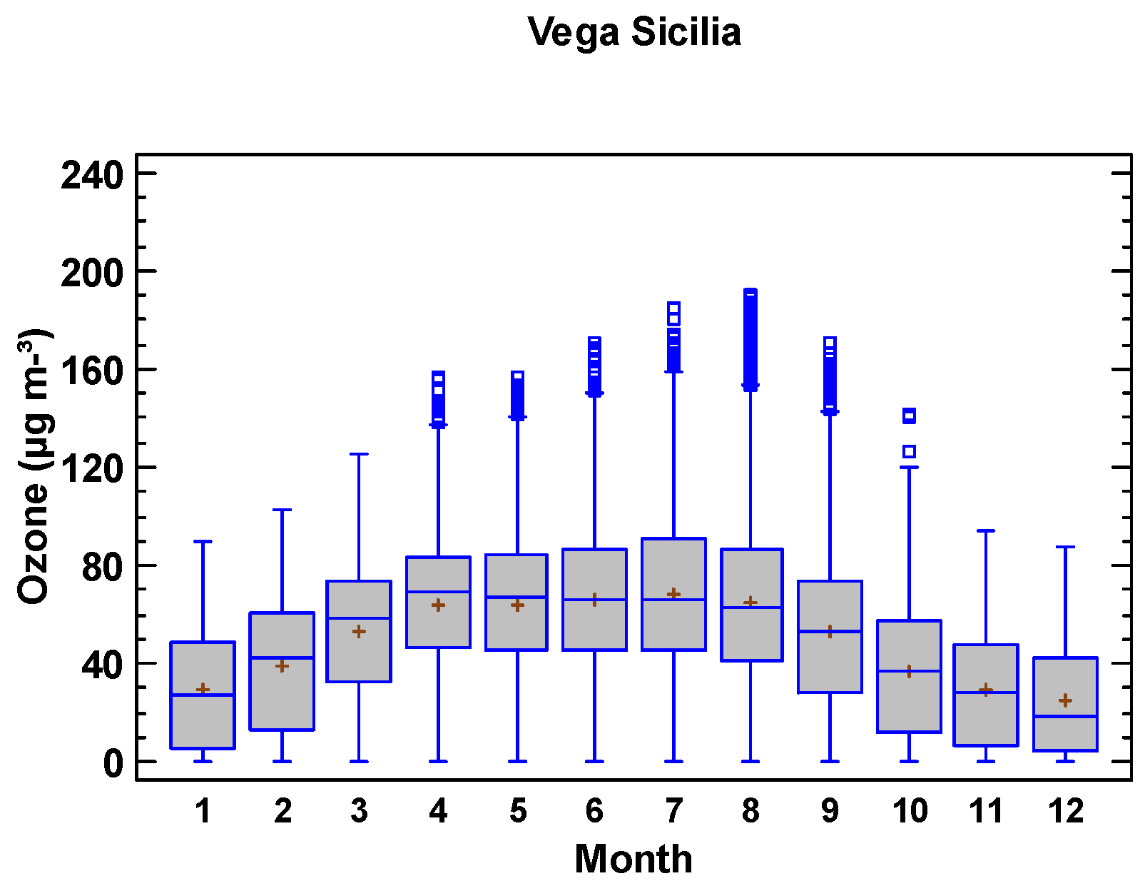
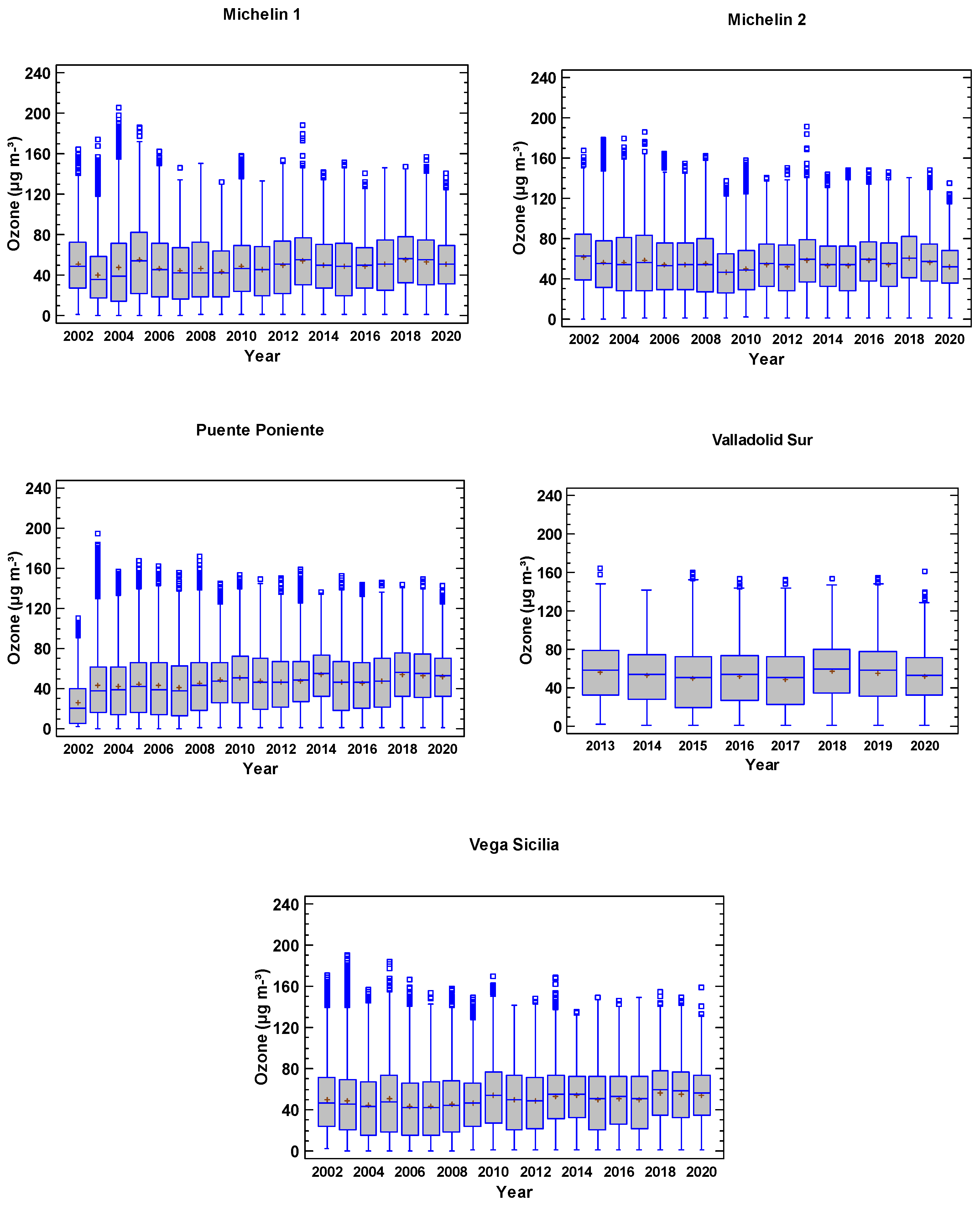
The year-to-year comparison for the measuring stations can be analysed from the box and whisker plot of Figure 2. There are several components in the graph to assess the results obtained. Fifty percent of data are within the vertical box between the lower and upper quartiles. The upper and lower whiskers extend out to the extreme maximum and minimum values below or above 1.5 times the interquartile range from the first and third quartiles. Small squares correspond to outliers. The cross and horizontal lines inside the box represent the median and mean values, respectively. As can be seen from the graphs, the highest average values were obtained in 2018 for all the stations, with values ranging between 54.2 µg m⁻³ (Puente del Poniente) and 57.6 µg m⁻³ (Valladolid Sur), except at Michelín 2, with 62.2 µg m⁻³ in 2002. In general, high concentrations associated to outliers were found in 2003 for most measuring stations, excluding Valladolid Sur. In regard to the lowest mean values, there was no common year, with the lowest being 2003, 2009, 2017 and 2006 at Michelín 1, Michelín 2, Valladolid Sur and Vega Sicilia, respectively, with values between 40.4 and 49.1 µg m⁻³. The low number of data recorded in 2002 at Puente del Poniente probably conditioned the low mean value of ozone concentration.

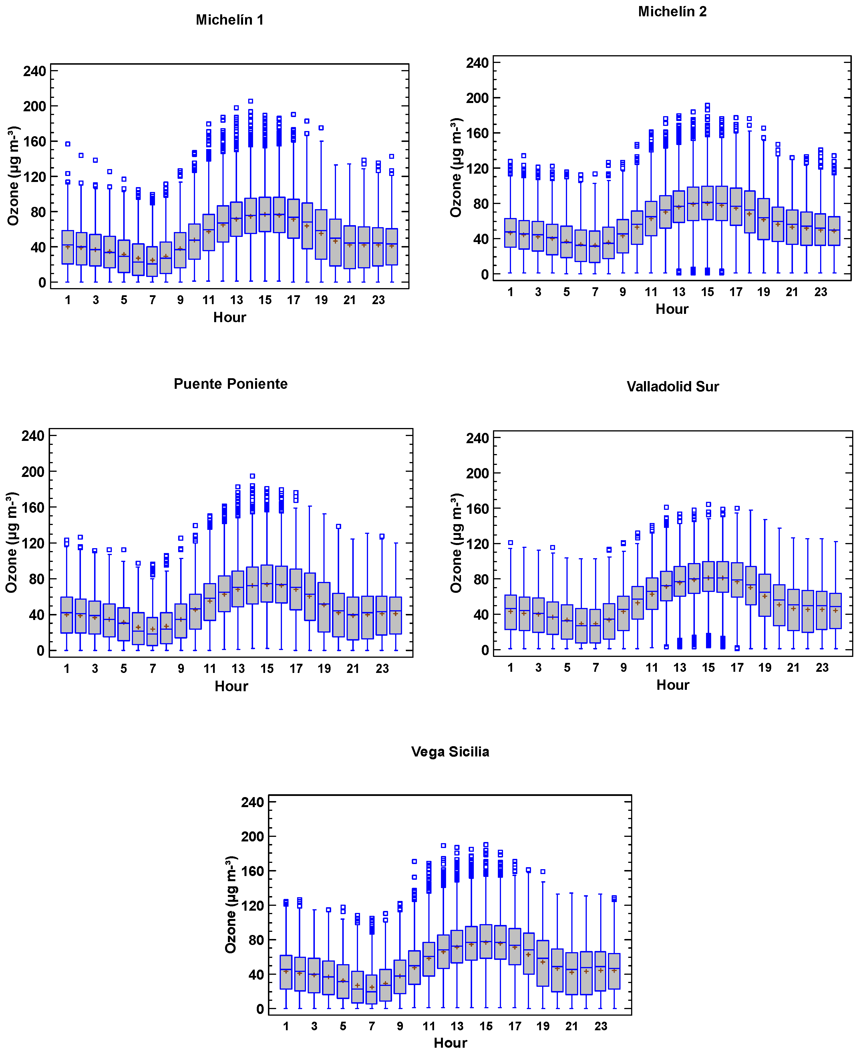
The daily evolution for the study period is depicted in Figure 3. The figure shows an increase in ozone concentrations in the morning, reaching the highest values from 14:00 to 16:00 GMT, with the maximum being at 15:00 GMT. The daily maximum was reached at a time when temperature and solar radiation presented high values. Mean values ranged between 73.8 and 80.9 µg m⁻³ at Puente del Poniente and Valladolid Sur, respectively. This increase during the day is mainly attributed to ozone production due to photochemical reactions in the boundary layer and transport from upper layers depending on solar radiation [2]. Ozone concentration then decayed until 20:00 GMT, and was followed by steady behaviour. Finally, the concentration decreased until the period 6:00–8:00 GMT, registering a minimum at 7:00 GMT, with mean values ranging between 23.4 µg m⁻³ at Puente del Poniente and 32.3 µg m⁻³ at Michelín 2. This result could be attributed to the ozone deposition and titration reaction between nitric oxide and ozone at night [25,26]. In addition, a slight right skewness of the data pattern can be seen during the day, and which differs to that observed in early morning. The maximum and minimum concentrations found were lower than those obtained for a short period at a measuring station located 32 km from Valladolid to the SE [26], which is considered a rural station. It is far from sources of precursors that reduce ozone and as expected, higher ozone values were observed.

Figure 2. Yearly evolution of ozone concentrations at each measuring station in the study period.

Figure 2. Yearly evolution of ozone concentrations at each measuring station in the study period.

Figure 3. Hourly evolution of ozone concentrations at each measuring station in the study period.

Figure 3. Hourly evolution of ozone concentrations at each measuring station in the study period.

The monthly mean pattern over the study period is shown in Figure 4 on an hourly basis, and is similar to those recorded at Mediterranean locations [26,27]. Ozone levels increased during the first months of the year for all the measuring stations, and reached the maximum value in July, which is mainly associated with the photochemical period [28] characterised by dry and sunny weather conditions. There was a secondary peak in May and June whose origin is not as clear. It might be related to stratospheric–tropospheric interchange, which generally occurs between January and June, the increase in solar radiation and the long-range transport of ozone [2,12,29]. Data variability was higher between April and August, and especially in July with the greatest interquartile range, around 47 µg m⁻³. Many outliers were obtained in spring and summer months, except at Valladolid Sur. After also evidencing high values in August, concentrations then decreased until the end of the year. The highest mean monthly ozone concentrations ranged between 66.7 µg m⁻³ at Puente del Poniente and 73.8 µg m⁻³ at Valladolid Sur. The seasonal variation found in ozone for the measuring stations can be associated to different factors, mainly local conditions within the city. Average mean values for the secondary peak were about 69 µg m⁻³ at Michelín 2 and Valladolid Sur, 65 µg m⁻³ at Michelín 1 and Vega Sicilia, and 63 µg m⁻³ at Puente del Poniente. The lowest levels, around 28 µg m⁻³ at Michelín 2 and 24 µg m⁻³ for the rest of the stations, were found in December.

Council Directive 97/72/EEC [30] on air pollution by ozone and Royal Decree-Law 102/2011 [31] regarding the improvement of air quality establish 180 µg m⁻³ as the information threshold based on a one-hour average concentration. During the study period, the threshold mentioned was exceeded only on a few occasions: Puente del Poniente on three occasions in 2003; the same number at Michelín 2, in 2005 and 2013; Vega Sicilia on eight occasions in July and August 2003 and 2005; Michelín 1 exceeded the limit twenty times in 2004, 2005 and 2013. In contrast, Valladolid Sur never surpassed the limit. These results reveal an acceptable level of ozone air quality in regard to the size of the city and its traffic density.

• Limit for the protection of human health

The limit for the protection of human health is 120 µg m⁻³ maximum daily value of an 8 h/day mean, and must not be exceeded on an average of more than 25 days per year over three years, as of 2010.

Table 3. Exceedance days of the human threshold value for ozone for each year and measuring site from 2010. (Values with * correspond to the number of days in that year).

Year/Station	Michelín 1	Michelín 2	Puente Poniente	Valladolid Sur	Vega Sicilia
2010	11	13	14		15
2011	7	6	11		15
2012	11	7	10		16
2013	12	9	8	15 *	12
2014	12	10	7	12 *	10
2015	14	13	10	17	12
1016	9	14	8	16	9
2017	11	14	8	16	10
2018	7	10	5	14	7
2019	11	8	7	19	8
2020	10	6	6	15	7

contains the number of exceedances for the protection of human health. Results confirm that, in general, the limit was not exceeded at any measuring site. This is particularly important with regard to the air quality of the city and the protection of the population’s health.

• Limit for the protection of vegetation

Following the same regulations for the protection of vegetation and the calculation procedure [30], the Accumulated Ozone exposure over a Threshold of 40 parts per billion, AOT40, was obtained for each measuring station in the study period. The limit value between May, June and July must not exceed 18,000 µg m⁻³ × h on average in a five-year period from 2010. The results corresponding to each year from 2010 presented in

Table 4. Limit of vegetation protection (AOT40) on the five-year average (µg m⁻³ × h).

Year/Station	Michelín 1	Michelín 2	Puente Poniente	Valladolid Sur	Vega Sicilia
2010	8094.2	10,463.4	11,186.8		9175.4
2011	7608.2	9265.8	10,374.6		9938.8
2012	9339.4	9121.0	10,517.6		10,254.8
2013	9182.6	8600.6	9952.2		10,569.6
2014	10,304.8	10,045.6	10,303.8		11,281.0
2015	12,154.8	12,585.4	10,489.4		11,167.0
2016	12,059.4	13,493.8	10,279.8		10,993.4
2017	12,127.4	13,827.4	10,290.6	14,008.2	11,509.2
2018	12,615.4	13,400.6	10,746.4	14,305.2	11,221.8
2019	13,455.2	13,816.4	11,536.8	15,084.0	11,641.0
2020	11,301.4	10,797.8	10,069.8	13,244.8	10,499.2

allow us to conclude that the threshold value was not surpassed at any location, yielding the last five-year average, 11,301.4, 10,797.8, 10,069.8, 13,244.8, 10,499.2 µg m⁻³ × h at Michelín 1, Michelín 2, Puente del Poniente, Valladolid Sur, and Vega Sicilia, respectively. A positive trend was found from 2010, although the AOT40 in 2020 decreased to values comparable to the averages obtained between 2012–2014.

3.2. Relationship between Ozone and Nitrogen Oxides

Ozone is not emitted directly into the atmosphere but is formed by chemical reactions of precursors such as nitric oxide (NO) and nitrogen dioxide (NO₂). Mean NO levels in the study period ranged between 6.9 and 13.5 µg m⁻³ (maximum up to 499 µg m⁻³). Mean NO₂ levels were within the interval 15.9 to 24.5 µg m⁻³ (maximum values below 351 µg m⁻³). Nitrogen oxide concentrations were similar at Vega Sicilia and Puente del Poniente, with mean values around 13 and 23 µg m⁻³ for NO and NO₂, respectively. However, concentrations were lower at Michelín 2 because it is of the industrial type and is located in the suburban area; these were NO with 6.9 µg m⁻³ and NO₂ with 16.5 µg m⁻³. Daily evolution of nitrogen oxides showed that maximum concentrations of NO and NO₂ were recorded in the morning, 8:00 GMT, and at night, 20:00 GMT. The highest hourly average of NO concentrations ranged between 14.6 and 27.7 µg m⁻³, and were recorded in the morning at Michelín 2 and Vega Sicilia, respectively. The interval at night ranged from 7.5 to 23.3 µg m⁻³ for the same measuring stations. The highest hourly mean NO₂ concentrations in the morning were between 21.2 and 32.5 µg m⁻³, and were obtained at Michelín 2 and Puente del Poniente, respectively. At night, those concentrations were 20.8 and 40.3 µg m⁻³, respectively.

The relationship between concurrent values of ozone and those compounds were established by a linear regression of the monthly averages. The Pearson correlation coefficients for each measuring station are shown in

Table 5. Pearson correlation coefficients between monthly ozone concentrations and NO and NO₂ for each measuring station at a 95% confidence level.

Station (O3)	NO	NO2
Michelín 1	−0.4330	−0.6557
Michelín 2	−0.4505	−0.6230
Puente Poniente	−0.4302	−0.7242
Valladolid Sur	−0.5455	−0.7426
Vega Sicilia	−0.5271	−0.7079

. The correlation between O₃ and NO₂ is negative, with values of the correlation coefficients greater than −0.6, prominent amongst which is Valladolid Sur with −0.7426. However, the relationship between O₃ and NO for each station presented slightly lower correlation coefficient values, above −0.4, with the highest coefficient at Valladolid Sur, −0.5455. Results showed that ozone is negatively correlated with nitrogen oxides. These correlations were attributed to the fact that the high ozone concentration was linked to the low level of nitrogen oxides as they are its precursors involved in photochemical reactions [32]. Differences found in the correlation coefficients between stations were therefore not very high but might be influenced by local conditions and by the fact that nitrogen oxides have decreased over the last few years.

3.3. Influence of Meteorology on Ozone Concentrations

Concentrations of air pollutants are influenced by the state of the atmosphere. Pearson correlation coefficients between monthly ozone concentrations and meteorological parameters, temperature and wind speed, were calculated for the study period (see

Table 6. Pearson correlation coefficients between ozone concentrations and meteorological variables for each measuring station at a 95% confidence level.

Station (O3)	Correlation Coefficient (Temperature)	Correlation Coefficient (Wind Speed)
Michelín 1	0.695	0.341
Michelín 2	0.703	0.331
Puente Poniente	0.736	0.344
Valladolid Sur	0.725	0.401
Vega Sicilia	0.734	0.336

). Results showed a moderate and significant linear relationship between ozone and surface air temperature linked to the photochemical reactions that produce ozone. Coefficients were above 0.7 for each station, such that the relationship is also conditioned by other atmospheric features such as humidity [25]. Tropospheric ozone is involved in oxidation processes to form hydroxyl radical, among others, which causes its destruction [33,34]. High levels of ozone in the study period were associated to higher temperatures that usually correspond to lower humidity and high solar radiation [35]. The relationship established the importance of temperature in ozone formation rates, which may be the main parameter used to determine ozone episodes [36].

Changes in wind speed condition the formation and dispersion of ozone [37]. A linear regression between them was applied. The relationship between ozone concentration and wind speed is weak and positive, with Pearson correlation coefficients ranging from 0.3 to 0.4, although these were statistically significant at a 95% confidence level. The relationship found suggested that high wind speed was associated with high levels of ozone. During the day, the increase in ozone concentrations is due to the combination of photochemical reaction, boundary layer processes and local wind patterns. The boundary layer would act on ozone variability since its height increases at noon due to convective heating and causes a stratified layer. The air in the lower heights, which has a lower ozone concentration, mixes with the air in the higher heights, which is probably richer in ozone [38]. Moreover, the local daily wind pattern is characterised by greater values of this parameter during the day, coinciding with the period of photochemical formation of ozone [3,38]. Other studies have found that the increase in wind speed influences mixing, dispersion and transport of ozone, resulting in a negative relationship [35,37].

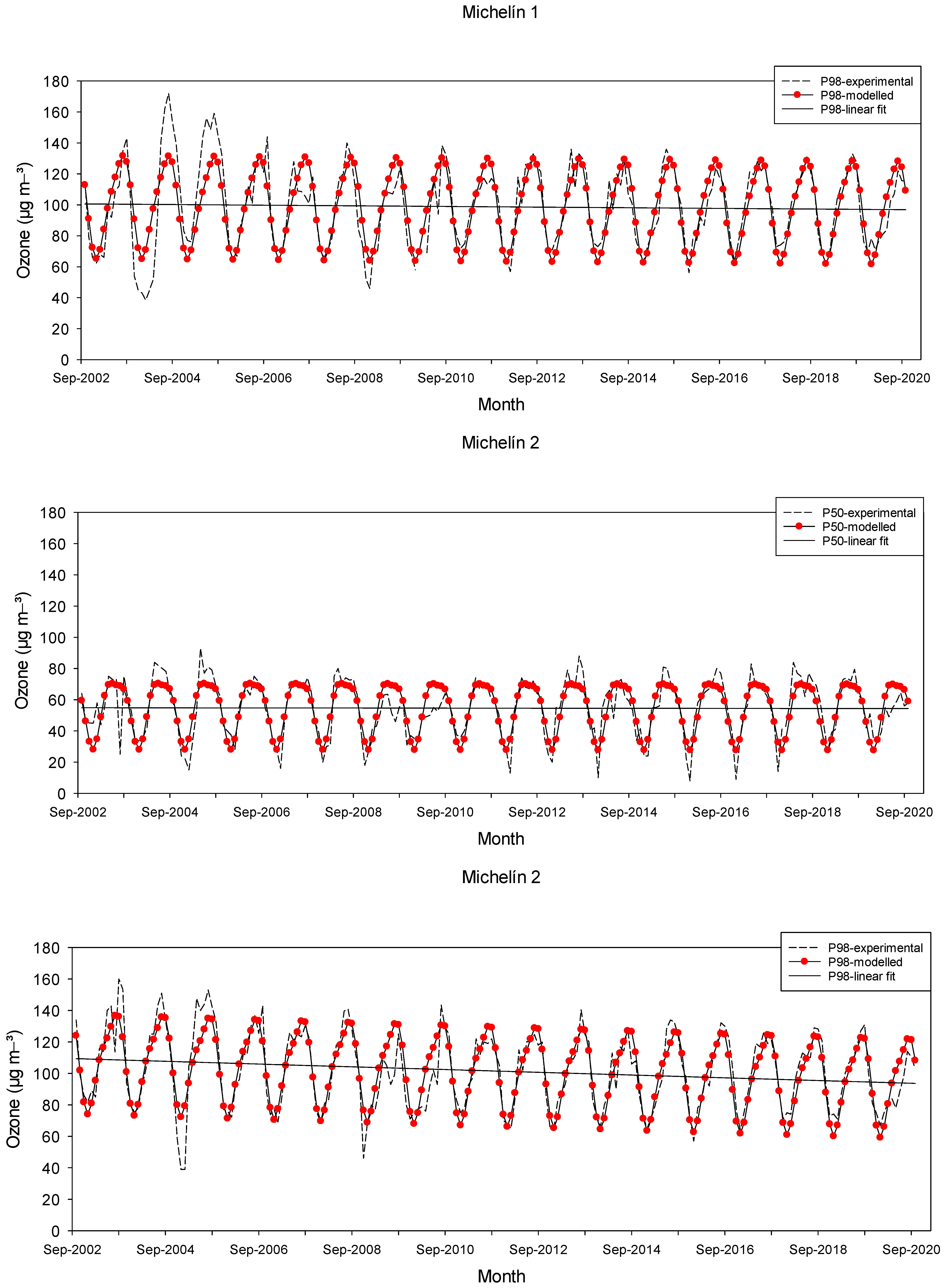
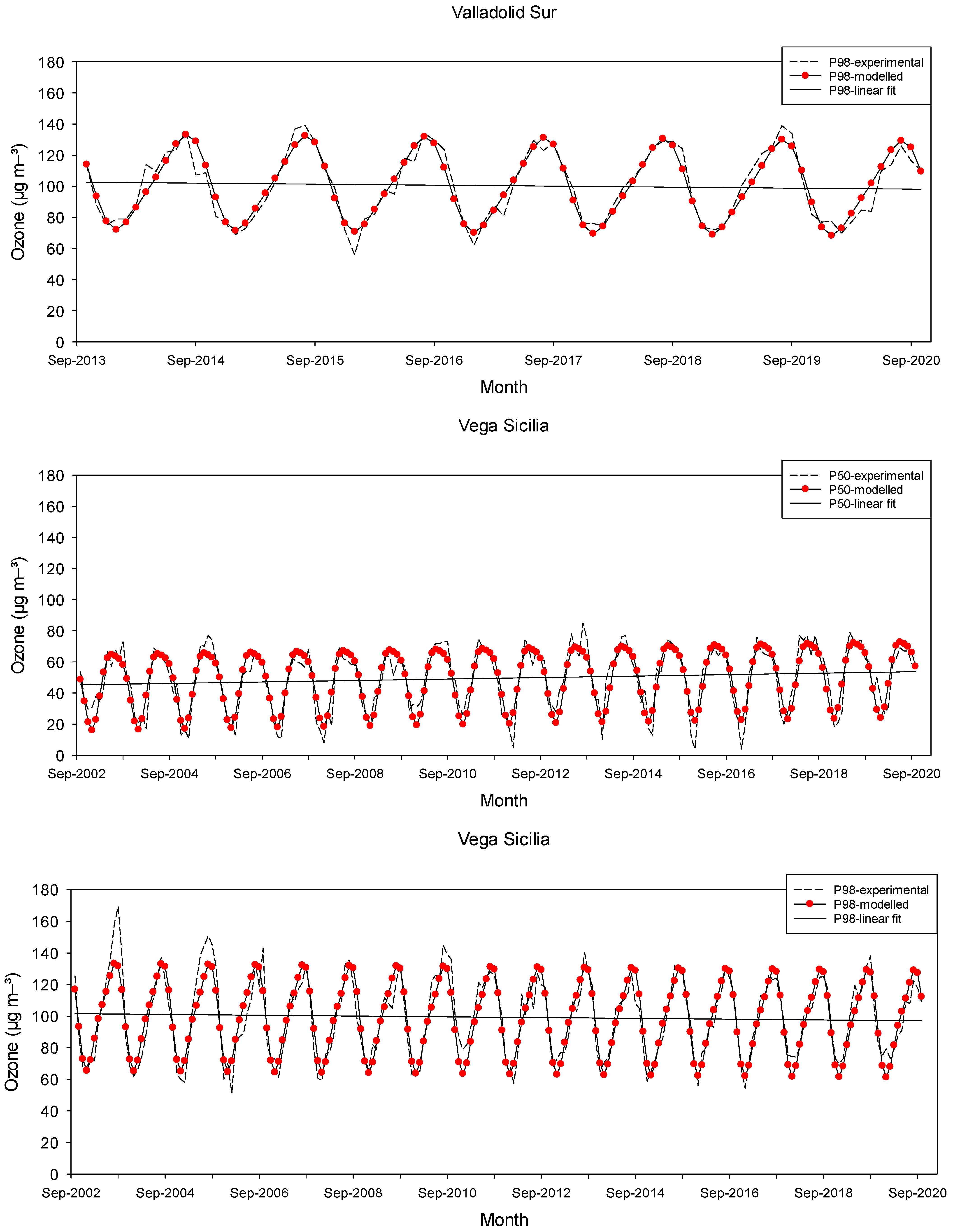
3.4. Ozone Concentration Trend

A further analysis of the monthly values for the mean and main percentiles (50th, 95th and 98th) was performed using a harmonic model from September 2002 to September 2020 (from September 2013 for Valladolid Sur). Equation (2) provides an analysis of ozone concentration trends. The coefficients of determination of the multiple regression and the b coefficient which represents the time variation of the ozone concentration per month over the study period are presented in Table 7 for each station. Figure 5 only depicts the temporal evolution of the 95th and 98th percentiles of the ozone concentrations. Experimental and modelled values are represented in addition to the linear fit. The results showed coefficients of determination higher than 80% at most stations and indicators, except at Michelín 1 and Michelín 2, although they were not below 70%. There was a significant relationship between variables, with a 95% confidence level. In general, increasing interannual rates were found for the mean, except at Michelín 2 and Valladolid Sur, which evidenced the opposite. Trend values of the mean concentration of ozone associated to the b parameter ranged from 0.029 µg m⁻³ month⁻¹ at Michelín 1 to 0.041 µg m⁻³ month⁻¹ at Puente del Poniente. The decreasing trend value in Michelín 2 was much lower, −0.006 µg m⁻³ month⁻¹, and −0.010 µg m⁻³ month⁻¹ at Valladolid Sur. The 50th percentile increased at a similar rate at Michelín 1 and Vega Sicilia, 0.035 and 0.039, µg m⁻³ month⁻¹, was slightly higher at Puente del Poniente, 0.054 µg m⁻³ month⁻¹, and was nearly steady at Michelín 2, −0.002 µg m⁻³ month⁻¹, and Valladolid Sur, 0.004 µg m⁻³ month⁻¹. A decreasing trend was found for the 95th and 98th percentiles. The b values associated to the 95th percentiles were insignificant at Michelín 1, Puente del Poniente and Vega Sicilia. However, they were −0.056 and −0.048 µg m⁻³ month⁻¹ at Michelín 2 and Valladolid Sur. The same behaviour was seen for the 98th percentile, −0.073 and −0.053 µg m⁻³ month⁻¹, respectively. These results concur with research using monitoring data from the United Kingdom, which have revealed that maximum ozone concentrations have decreased by around 30% over the last decade. Reports for other sites in Europe and North America have also been consistent with the decrease in peak values. Nevertheless, in contrast, the increase in the yearly mean concentration, 0.1 ppb year⁻¹, was also confirmed [39,40,41].

The long-term trends are different mainly for the stations that are further outside the city, such as Valladolid Sur and Michelín 2 regarding the high percentiles, 95th and 98th, with a significant decrease compared to that for the other measuring stations. In general, the combination of regional and local effects around the stations conditioned the results, thereby evidencing their importance in the generation, reduction and transport of ozone. Moreover, results indicated that emission control measures could prove effective in reducing high ozone concentrations [42,43].

Table 7. Coefficients of determination (%) and b (µg m⁻³ month⁻¹) of the multiple regression fit in the study period for each measuring station.

	Michelín 1		Michelín 2		Puente Poniente		Valladolid Sur		Vega Sicilia
	R2	b	R2	b	R2	b	R2	b	R2	b
Mean	79.5	0.029	77.9	−0.006	88.2	0.041	82.6	−0.010	86.9	0.034
50th percentile	75.7	0.035	71.6	−0.002	83.6	0.054	74.6	0.004	82.1	0.039
95th percentile	74.2	−0.003	80.1	−0.056	86.5	0.004	89.0	−0.048	86.9	−0.007
98th percentile	74.1	−0.017	79.7	−0.073	85.0	−0.021	90.4	−0.053	85.6	−0.021

Table 7. Coefficients of determination (%) and b (µg m⁻³ month⁻¹) of the multiple regression fit in the study period for each measuring station.

	Michelín 1		Michelín 2		Puente Poniente		Valladolid Sur		Vega Sicilia
	R2	b	R2	b	R2	b	R2	b	R2	b
Mean	79.5	0.029	77.9	−0.006	88.2	0.041	82.6	−0.010	86.9	0.034
50th percentile	75.7	0.035	71.6	−0.002	83.6	0.054	74.6	0.004	82.1	0.039
95th percentile	74.2	−0.003	80.1	−0.056	86.5	0.004	89.0	−0.048	86.9	−0.007
98th percentile	74.1	−0.017	79.7	−0.073	85.0	−0.021	90.4	−0.053	85.6	−0.021

Figure 5. Evolution of the monthly ozone concentrations of the 50th percentile (P50) and 98th percentile (P98) in the study period.

Figure 5. Evolution of the monthly ozone concentrations of the 50th percentile (P50) and 98th percentile (P98) in the study period.

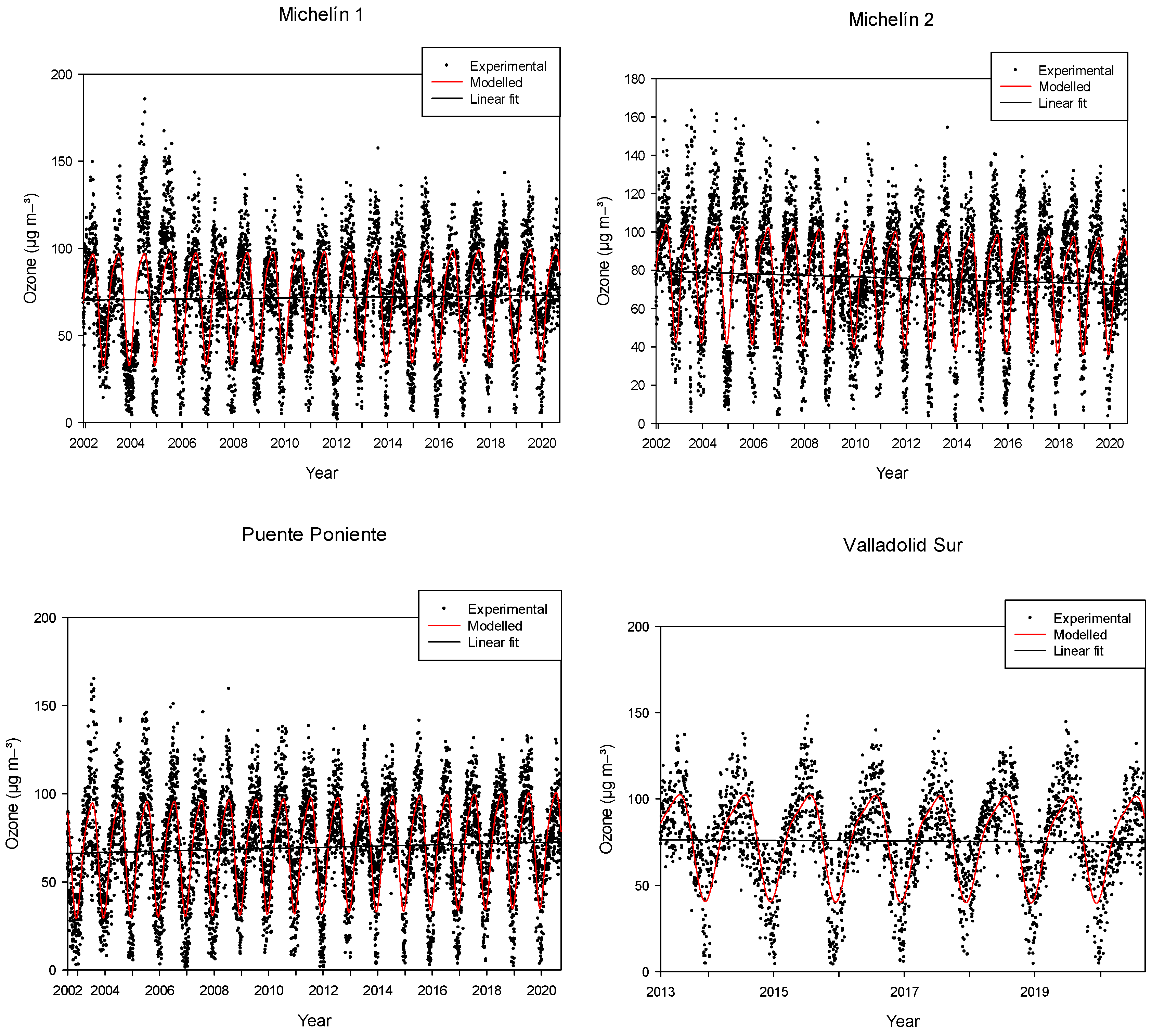
A similar procedure was applied for the maximum daily 8 h average of ozone, but with using t as the time in consecutive days and ω the frequency 2π/365.242 (rad day⁻¹) and was also analysed for each station. The evolution of this indicator in the study period is shown in Figure 6. Although the coefficients of determination were between 57.8 and 64.6% for Michelín 2 and Puente del Poniente, respectively, they were statistically significant at a 95% confidence level. The trend was negative for Michelín 2 (−0.001 µg m⁻³ day⁻¹) and Valladolid Sur (−0.0004 µg m⁻³ day⁻¹). However, ozone concentrations increased for the rest of the stations. The trend value was greater for the measuring station located further inside the city, Puente del Poniente, around 0.0009 µg m⁻³ day⁻¹, and a less strong increase, up to 0.0005 µg m⁻³ day⁻¹, was obtained for Michelín 1 and Vega Sicilia.

4. Conclusions

A study of ozone concentrations over 18 years, from 2002 to 2020, was carried out at five air measuring stations in an urban area, Valladolid, in northern Spain. Levels of its precursors and specific meteorological conditions were seen to influence the levels of ozone found. The overall mean ozone value on an hourly basis was around 50 µg m⁻³ at most stations, except Valladolid Sur and Michelín 2, which had a mean value of around 3 and 5 µg m⁻³ higher, respectively. The overall median value was 1 µg m⁻³ higher than the mean values at all stations. The maximum concentration was 205 µg m⁻³, and was recorded at Michelín 1. However, the maximum at Valladolid Sur was 164 µg m⁻³. The interquartile range (IQR), close to 48 µg m⁻³, was similar at all stations. The 98th percentile values ranged between 115 and 120 µg m⁻³. A wide range of mean maximum concentrations from spring to summer was evident. The primary peak was obtained in July, with temperature being the determinant factor, and ranged from 66.7 µg m⁻³ at Michelín 1 to 73.8 µg m⁻³ at Valladolid Sur. The secondary peak occurred in spring, from May–June, and was around 69 µg m⁻³ at Valladolid Sur and Michelín 2, and around 65 µg m⁻³ at the remaining stations, and was favoured by ozone from ozone stratospheric intrusions. Daily ozone patterns showed the highest levels of this pollutant, mainly at 15:00 h, with values between 73.8 and 80.9 µg m⁻³ at Puente del Poniente and Valladolid Sur, respectively, supporting the idea that photochemical processes govern ozone generation. Low ozone concentrations occurred at night and in the early morning, and reached the lowest values at 7:00 h, with values from 23.4 to 32.3 µg m⁻³ at Puente del Poniente and Michelín 2, respectively, related to the reduction by NO reactions and deposition processes.

Results show that ozone concentration variability can largely be explained by negative linear dependence with precursor concentrations (NO_x), yielding Pearson correlation coefficients of around 0.5 for NO at most measuring stations, and 0.7 for NO₂. The differences found between stations were not noticeable but might be influenced by local features.

The relationship between meteorological parameters and ozone concentrations also indicated the importance of their changes in the troposphere. A strong correlation was found for temperature, with correlation coefficients above 0.7, showing that ozone levels in the study period were linked to high temperature and solar radiation. However, a positive and weak relationship was found for wind speed, indicating that ozone variability was poorly explained by this meteorological parameter.

Evaluation of the urban air quality of the study area in accordance with regulatory standards confirmed that only on rare occasions did ozone levels exceed current air quality regulations, which establish 180 µg m⁻³ as the information threshold. Moreover, the threshold for the protection of human health, 120 µg m⁻³, was not exceeded at any measuring site. This is of particular importance with regard to tropospheric ozone pollution in the city and the protection of the population’s health. The last five-year average of AOT40 did not surpass the limit for the protection of vegetation. The results can help to improve current knowledge of the temporal variability and ozone trend in southern Europe.

Inter-annual trends of the 95th percentile and 98th percentile were negative at all the measuring stations, with significant values of −0.056 and −0.073 µg m⁻³ month⁻¹ at Michelín 2 and −0.048 and −0.053 µg m⁻³ month⁻¹ at Valladolid Sur, respectively. Lower values were found for the 98th percentile decrease at Michelín 1 and Puente del Poniente, −0.017 and−0.021 µg m⁻³ month⁻¹. Moreover, the trend for the maximum daily 8 h average also decreased for Michelín 2 and Valladolid Sur. The 50th percentile showed a low trend at Michelín 2 and Valladolid Sur, with the rest of the stations experiencing major changes during the study period of between 0.035 to 0.054 µg m⁻³ month⁻¹. Positive trends were obtained for the mean value, up to 0.041 µg m⁻³ month⁻¹, except at two stations, which displayed no significant results. This paper confirms that peak ozone levels have decreased over the last decade but that, in general, mean levels have increased slightly over the same period, with the corresponding implications that these ozone patterns have for human health and vegetation and which should be given consideration by the authorities.

References

1. Brönnimann, S.; Buchmann, B.; Wanner, H. Trends in near-surface ozone concentrations in Switzerland: The 1990s. Atmos. Environ. 2002, 36, 2841–2852. [Google Scholar] [CrossRef]
2. García, M.A.; Sánchez, M.L.; Pérez, I.A.; de Torre, B. Ground level ozone concentrations at a rural location in northern Spain. Sci. Total Environ. 2005, 348, 135–150. [Google Scholar] [CrossRef] [PubMed]
3. De Torre, B. Perfiles Verticales de Ozono y del Coeficiente de Extinción. Contribución al Diagnóstico de la Calidad del Aire en Segovia. Ph.D. Thesis, University of Valladolid, Valladolid, Spain, 2015. [Google Scholar]
4. Monteiro, A.; Strunk, A.; Carvalho, A.; Tchepel, O.; Miranda, A.I.; Borrego, C.; Saavedra, S.; Rodriguez, A.; Souto, J.; Casares, J.; et al. Investigating a high ozone episode in a rural mountain site. Environ. Pollut. 2012, 162, 176–189. [Google Scholar] [CrossRef] [PubMed]
5. Wang, Q.Y.; Gao, R.S.; Cao, J.J.; Schwarz, J.P.; Fahey, D.W.; Shen, Z.X.; Hu, T.F.; Wang, P.; Xu, X.B.; Huang, R.J. Observations of high level of ozone at Qinghai Lake basin in the northeastern Qinghai-Tibetan Plateau, western China. J. Atmos. Chem. 2015, 72, 19–26. [Google Scholar] [CrossRef]
6. Fatin, A.B.; Norliza, A.R.; Jarinah, A.A. Tropospheric ozone formation estimation in urban city, Bangay, using artificial neural network (ANN). Comput. Intell. Neurosci. 2019, 2019, 6252983. [Google Scholar]
7. Monks, P.S.; Archibald, A.T.; Colette, A.; Cooper, O.; Coyle, M.; Derwent, R.; Fowler, D.; Granier, C.; Law, K.S.; Mills, G.E.; et al. Tropospheric ozone and its precursors from the urban to the global scale from air quality to short-lived climate forcer. Atmos. Chem. Phys. 2015, 15, 8889–8973. [Google Scholar] [CrossRef] [Green Version]
8. OMM. Boletín Sobre los Gases de Efecto Invernadero; Organización Meteorológica Mundial: Geneva, Switzerland, 2017. [Google Scholar]
9. WMO. Bulletin Reactive Gases. Highlights from the Global Atmosphere Watch Programme; World Meteorological Organization: Geneve, Switzerland, 2018. [Google Scholar]
10. Prados-Roman, C.; Cuevas, C.A.; Fernandez, R.P.; Kinnison, D.E.; Lamarque, J.F.; Saiz-Lopez, A. A negative feedback between anthropogenic ozone pollution and enhanced ocean emissions of iodine. Atmos. Chem. Phys. 2015, 15, 2215–2224. [Google Scholar] [CrossRef] [Green Version]
11. Nishimura, H.; Shimadera, H.; Kondo, A.; Bao, H.; Shrestha, K.; Inoue, Y. Evaluation of light dependence of monoterpene emission and its effect on surface ozone concentration. Atmos. Environ. 2015, 104, 143–153. [Google Scholar] [CrossRef]
12. Monks, P.S. A review of the observations and origins of the spring ozone maximum. Atmos. Environ. 2000, 34, 3545–3561. [Google Scholar] [CrossRef]
13. Gong, C.; Liao, H. A typical weather pattern for ozone pollution events in North China. Atmos. Chem. Phys. 2019, 19, 13725–13740. [Google Scholar] [CrossRef] [Green Version]
14. Han, H.; Liu, J.; Shu, L.; Wang, T.; Yuan, H. Local and synoptic meteorological influences on daily variability in summertime surface ozone in eastern China. Atmos. Chem. Phys. 2020, 20, 203–222. [Google Scholar] [CrossRef] [Green Version]
15. Tang, G.; Zhang, J.; Zhu, X.; Song, T.; Münkel, C.; Hu, B.; Schäfer, K.; Liu, Z.; Zhang, J.; Wang, L.; et al. Mixing layer height and its implications for air pollution over Beijing, China. Atmos. Chem. Phys. 2016, 16, 2459–2475. [Google Scholar] [CrossRef] [Green Version]
16. Geiß, L.; Wiegner, M.; Bonn, B.; Schäfer, K.; Forkel, R.; Schneidemesser, E.; Münkel, C.; Chan, K.L.; Nothard, R. Mixing layer height as an indicator for urban air quality? Atmos. Meas. Tech. 2017, 10, 2969–2988. [Google Scholar] [CrossRef] [Green Version]
17. Hastie, D.R.; Narayan, J.; Sciller, C.; Niki, H.; Hepson, P.B.; Sills, D. Observational evidence for the impact of the lake breeze circulation on ozone concentrations in Southern Ontario. Atmos. Environ. 1999, 33, 323–335. [Google Scholar] [CrossRef] [Green Version]
18. Brankov, E.; Henry, R.; Civerolo, K.; Hao, W.; Rao, S.T.; Misra, P.K.; Bioxam, R.; Reid, N. Assessing the effects of transboundary ozone pollution between Ontario, Canada and New York, USA. Environ. Pollut. 2003, 123, 403–411. [Google Scholar] [CrossRef]
19. The Royal Society. Ground-Level Ozone in the 21st Century: Future Trends, Impacts and Policy Implications. Science Policy Report. 15 August 2008. Available online: https://royalsociety.org/-/media/Royal_Society_Content/policy/publications/2008/7925.pdf (accessed on 10 October 2021).
20. Paoletti, E.; de Marco, A.; Beddows, D.C.S.; Harrison, R.M.; Manning, R.M. Ozone levels in European and USA cities are increasing more than at rural sites, while peak values are decreasing. Environ. Pollut. 2014, 192, 295–299. [Google Scholar] [CrossRef]
21. Sicard, P.; Paoletti, E.; Agathokleous, E.; Araminiene, V.; Proietti, C.; Coulibaly, F.; De Marco, A. Ozone weekend effect in cities: Deep insights for urban air pollution control. Atmos. Res. 2020, 191, 110193. [Google Scholar] [CrossRef]
22. Zhang, Z.; Zhang, X.; Gong, D.; Quan, W.; Zhao, X.; Ma, Z.; Kim, S.J. Evolution of surface O3 and PM2.5 concentrations and their relationships with meteorological conditions over the last decade in Beijing. Atmos. Environ. 2015, 108, 67–75. [Google Scholar] [CrossRef]
23. Xing, J.; Mathur, R.; Pleim, J.; Hogrefe, C.; Gan, C.M.; Wong, D.C.; Wei, C.; Gilliam, R.; Poulio, G. Observations and modelling of air quality over 1990–2010 across de Northern Hemisphere: China, the United States and Europe. Atmos. Chem. Phys. 2015, 15, 2723–2747. [Google Scholar] [CrossRef] [Green Version]
24. Junta de Castilla y León. Atlas Agroclimático, Castilla y León; Junta de Castilla y León: León, Spain, 2013. [Google Scholar]
25. Dueñas, C.; Fernández, M.C.; Cañete, S.; Carretero, J.; Liger, E. Assessment of ozone variations and meteorological effects in an urban area in the Mediterranean Coast. Sci. Total Environ. 2002, 299, 97–113. [Google Scholar] [CrossRef]
26. Sánchez, M.L.; García, M.A.; Pérez, I.A.; de Torre, B. Evaluation of surface ozone measurements during 2000–2005 at a rural area in the upper Spanish plateau. J. Atmos. Chem. 2008, 60, 137–152. [Google Scholar] [CrossRef]
27. Nolle, M.; Ellul, R.; Heinrich, G.; Gqsten, H. A long-term study of background ozone concentrations in central Mediterranean—Diurnal and seasonal variations on the island of Gozo. Atmos. Environ. 2002, 36, 1391–1402. [Google Scholar] [CrossRef]
28. Ribas, A.; Peñuelas, J. Temporal patterns of surface ozone levels in different habitats of the north western Mediterranean basin. Atmos. Environ. 2004, 38, 985–992. [Google Scholar] [CrossRef]
29. Vingarzan, R. A review of surface ozone background levels and trends. Atmos. Environ. 2004, 38, 3431–3442. [Google Scholar] [CrossRef]
30. European Union. Directive 2002/3/EC of the European Parliament and of the Council relating to ozone in ambient air. Off. J. Eur. Community 2002, L67, 14–30. [Google Scholar]
31. BOE. Real Decreto 102/2011, de 28 de Enero, Relativo a la Mejora de la Calidad del Aire. 2011. Available online: https://www.boe.es/boe/dias/2011/01/29/pdfs/BOE-A-2011-1645.pdf (accessed on 2 September 2021).
32. Hashim, N.I.; Yusoff, N.A.; Noor, N.M.; Ul-Saufie, A.Z. Assessment of surface ozone concentration in Northern Peninsular Malaysia. IOP Conf. Ser. Mater. Sci. Eng. 2019, 551, 012100. [Google Scholar] [CrossRef] [Green Version]
33. Londhe, A.L.; Jadhav, D.B.; Buchunde, P.S.; Kartha, M.J. Surface ozone variability in the urban and nearby rural locations of tropical India. Curr. Sci. 2008, 95, 1723–1729. [Google Scholar]
34. Cano, J.N.; Morales, J.A.; Sánchez, J.; Colina, M.N.; Torres, J.C. Evaluación de los niveles de ozono en la ciudad de Maracaibo, estado Zulia, Venezuela. Rev. Int. Contam. Ambie. 2016, 32, 25–34. [Google Scholar]
35. Kovač-Andriċ, E.; Radanovċ, T.; Topaloviċ, I.; Markoviċ, B.; Sakač, N. Temporal Variations in Concentrations of Ozone, Nitrogen Dioxide, and Carbon Monoxide at Osijek, Croatia. Hindawi Publishing Corporation. Adv. Meteorol. 2013, 2013, 469786. [Google Scholar] [CrossRef]
36. Rubio, A.; Lissi, E. Temperature as thumb rule predictor of ozone levels in Santiago de Chile ground air. J. Chil. Chem. Soc. 2014, 59, 2427–2431. [Google Scholar] [CrossRef] [Green Version]
37. Venkitaswamy, S.; Bhaskar, V. Relationship between ozone with nitrogen dioxide and climatic impacts over major cities in India. Sustain. Environ. Res. 2015, 25, 295–304. [Google Scholar]
38. Lal, S.; Naja, M.; Subbaraya, B.H. Seasonal variations in surface ozone and its precursors over an urban site in India. Atmos. Environ. 2000, 34, 2713–2724. [Google Scholar] [CrossRef]
39. Coyle, M.; Fowler, D.; Ashmore, M. New Directions: Implications of increasing tropospheric background ozone concentrations for vegetation. Editorial. Atmos. Environ. 2003, 37, 153–154. [Google Scholar] [CrossRef]
40. Yan, Y.; Pozzer, A.; Ojha, N.; Lin, J.; Lelieveld, J. Analysis of European ozone trends in the period 1995–2014. Atmos. Chem. Phys. Discuss. 2017, 1–26. [Google Scholar] [CrossRef] [Green Version]
41. Yan, Y.; Lin, J.; He, C. Ozone trends over the United States at different times of day. Atmos. Chem. Phys. 2018, 18, 1185–1202. [Google Scholar] [CrossRef] [Green Version]
42. Massagué, J.; Contreras, J.; Campos, A.; Alastuey, A.; Querol, X. 2005–2018 trends in ozone peak concentration and spatial contributions in the Guadalquivir Valley, southern Spain. Atmos. Environ. 2021, 254, 118385. [Google Scholar] [CrossRef]
43. Cachón, J.; Canda, E.; David, R.A. Environmental Profile of Spain 2017. Indicator-Based-Report. Directorate-General for Biodiversity and Environmental Quality; Ministry for Ecological Transition: Madrid, Spain, 2019; pp. 1–345.
Figure 1. Location of the measuring stations in Valladolid (Castilla y León, Spain) (Image courtesy of Valladolid Council).
Atmosphere 12 01495 g001
Figure 4. Monthly evolution of ozone concentrations at each measuring station in the study period.
Atmosphere 12 01495 g004aAtmosphere 12 01495 g004b
Figure 6. Evolution of the maximum daily 8 h average ozone concentrations in the study period.
Atmosphere 12 01495 g006aAtmosphere 12 01495 g006b